Data and Computer
Dataand Computer
Communications
Communications
Eighth Edition
Eighth Edition
by William Stallings
by William Stallings
Chapter 12 –
Chapter 12 – Routing in Switched
Routing in Switched
Networks
Networks
2.
Routing
Routing in PacketSwitched Network
in Packet Switched Network
key design issue for (packet) switched networks
key design issue for (packet) switched networks
select route across network between end nodes
select route across network between end nodes
characteristics required:
characteristics required:
correctness
correctness
simplicity
simplicity
Robustness-ability of the n/w to deliver packets in face of
Robustness-ability of the n/w to deliver packets in face of
localized failure and overloads,
localized failure and overloads,
Stability- shift from one area to the 2
Stability- shift from one area to the 2nd
nd
,cause packet to travel in
,cause packet to travel in
loops.
loops.
Fairness high priority to exchange of packets between
Fairness high priority to exchange of packets between
Optimality near by stations , may unfair to station who want
Optimality near by stations , may unfair to station who want
to communicate to distant stations.
to communicate to distant stations.
Efficiency-transmission overhead which impairs network
Efficiency-transmission overhead which impairs network
efficency.
efficency.
3.
Performance Criteria
Performance Criteria
used for selection of route
used for selection of route
simplest is “minimum hop”
simplest is “minimum hop”
can be generalized as “least cost”
can be generalized as “least cost”
Cost is inversely related to the data rate or
Cost is inversely related to the data rate or
the current queuing delay on the link.
the current queuing delay on the link.
Least cost route should provide the highest
Least cost route should provide the highest
throughput
throughput
Least cost route should minimize delay.
Least cost route should minimize delay.
Decision Time andPlace
Decision Time and Place
time
time
Datagram packet –routing decision individually for each packet.
Datagram packet –routing decision individually for each packet.
Virtual circuit basis-routing decision made at the time the VC is
Virtual circuit basis-routing decision made at the time the VC is
established
established
fixed – if subsequent packet using that VC follow the same route.
fixed – if subsequent packet using that VC follow the same route.
Dynamically changing if route assigned to a particular VC changes
Dynamically changing if route assigned to a particular VC changes
in response to changing condition.
in response to changing condition.
place
place
distributed - made by each node
distributed - made by each node
centralized
centralized
source
source
6.
Decision Place
Decision Place
Which node or nodes in the n/w are
Which node or nodes in the n/w are
responsible for routing decesion.
responsible for routing decesion.
distributed – each node in the n/w is responsible
distributed – each node in the n/w is responsible
for the routing decision.(complex but robust)
for the routing decision.(complex but robust)
Centralized – routing decision made by a
Centralized – routing decision made by a
designated node = e,g n/w control centre.(loss of
designated node = e,g n/w control centre.(loss of
n/w control center may block operation of n/w)
n/w control center may block operation of n/w)
Source – routing decision made by source station
Source – routing decision made by source station
rather than by the node.
rather than by the node.
User can dictate route through the n/w that meets
User can dictate route through the n/w that meets
criteria local to the user.
criteria local to the user.
7.
N/w Information Source&Update Timing
N/w Information Source &Update Timing
routing decisions usually based on knowledge of n/w
routing decisions usually based on knowledge of n/w
topology, traffic load and link cost. (not always)
topology, traffic load and link cost. (not always)
distributed routing
distributed routing
• using local knowledge,(cost of outgoing link) info from adjacent
using local knowledge,(cost of outgoing link) info from adjacent
nodes, (amount of congestion at the node)info from all nodes on a
nodes, (amount of congestion at the node)info from all nodes on a
potential route
potential route
central routing
central routing
• collect info from all nodes
collect info from all nodes
issue of update timing
issue of update timing
when is network info held by nodes updated
when is network info held by nodes updated
Local information – continuously updated
Local information – continuously updated
Adjacent /all nodes
Adjacent /all nodes
fixed - never updated
fixed - never updated
adaptive - regular updates
adaptive - regular updates
8.
Routing Strategies -Fixed Routing
Routing Strategies - Fixed Routing
use a single permanent route for each source to
use a single permanent route for each source to
destination pair
destination pair
determined using a least cost algorithm
determined using a least cost algorithm
route is fixed
route is fixed
at least until a change in network topology
at least until a change in network topology
hence cannot respond to traffic changes
hence cannot respond to traffic changes
No difference for datagram and virtual circuits.
No difference for datagram and virtual circuits.
advantage is simplicity
advantage is simplicity
disadvantage is lack of flexibility- does not react
disadvantage is lack of flexibility- does not react
to network congestion or failures.
to network congestion or failures.
10.
Routing Strategies -Flooding
Routing Strategies - Flooding
At each node, an incoming packet is retransmitted on
At each node, an incoming packet is retransmitted on
all outgoing links except for the link on which it arrived.
all outgoing links except for the link on which it arrived.
Eventually
Eventually multiple copies arrive at destination
multiple copies arrive at destination
each packet is uniquely numbered so duplicates can
each packet is uniquely numbered so duplicates can
be discarded (VC no.,Seq no.,source node).
be discarded (VC no.,Seq no.,source node).
need some way to limit incessant retransmission
need some way to limit incessant retransmission
nodes can remember packets already forwarded to keep
nodes can remember packets already forwarded to keep
network load in bounds
network load in bounds
or include a hop count in packets
or include a hop count in packets
Properties of Flooding
Propertiesof Flooding
all possible routes are tried
all possible routes are tried
very robust used to send emergency messages
very robust used to send emergency messages
at least one packet will have taken minimum hop
at least one packet will have taken minimum hop
count route
count route
can be used to set up virtual circuit route
can be used to set up virtual circuit route
all nodes directly or indirectly are visited
all nodes directly or indirectly are visited
useful to distribute information (eg. routing)
useful to distribute information (eg. routing)
disadvantage is high traffic load generated
disadvantage is high traffic load generated
13.
Routing Strategies -Random
Routing Strategies - Random
Routing
Routing
simplicity of flooding with much less load
simplicity of flooding with much less load
node selects one outgoing path for
node selects one outgoing path for
retransmission of incoming packet
retransmission of incoming packet
selection can be random or round robin
selection can be random or round robin
a refinement is to select outgoing path based on
a refinement is to select outgoing path based on
probability calculation
probability calculation
no network info needed
no network info needed
but a random route is typically neither least cost
but a random route is typically neither least cost
nor minimum hop
nor minimum hop
14.
Routing Strategies -Adaptive Routing
Routing Strategies - Adaptive Routing
used by almost all packet switching networks
used by almost all packet switching networks
routing decisions change as conditions on the network
routing decisions change as conditions on the network
change due to failure or congestion
change due to failure or congestion
requires information about the state of the network
requires information about the state of the network
exchange between the nodes.
exchange between the nodes.
disadvantages:
disadvantages:
decisions more complex-process burden on n/w increases
decisions more complex-process burden on n/w increases
adaptive strategies depend on status information that is
adaptive strategies depend on status information that is
collected at one place but used at another
collected at one place but used at another.
. t
tradeoff between
radeoff between
quality of network info and overhead, more information ,
quality of network info and overhead, more information ,
more frequently exchanged, better routing decision.
more frequently exchanged, better routing decision.
reacting too quickly can cause oscillation
reacting too quickly can cause oscillation
reacting too slowly means info may be irrelevant
reacting too slowly means info may be irrelevant
15.
Adaptive Routing -
AdaptiveRouting -
Advantages
Advantages
An adaptive routing strategy can improve
performance, as seen by the network user.
• An adaptive routing strategy can aid in
congestion
Because an adaptive routing strategy tends to
balance loads, it can delay the onset of
severe congestion.
16.
Classification of Adaptive
Classificationof Adaptive
Routing Startegies
Routing Startegies
based on information sources
based on information sources
local (isolated)
local (isolated)
• route to outgoing link with shortest queue
route to outgoing link with shortest queue
• can include bias for each destination
can include bias for each destination
• Rarely used - does not make use of available info
Rarely used - does not make use of available info
adjacent nodes
adjacent nodes
• takes advantage on delay / outage info
takes advantage on delay / outage info
• distributed or centralized
distributed or centralized
all nodes
all nodes
• like adjacent
like adjacent
ARPANET Routing Strategies
ARPANETRouting Strategies
1st Generation
1st Generation
1969
1969
distributed adaptive using estimated delay
distributed adaptive using estimated delay
queue length used as estimate of delay
queue length used as estimate of delay
using Bellman-Ford algorithm
using Bellman-Ford algorithm
node exchanges delay vector with neighbors
node exchanges delay vector with neighbors
update routing table based on incoming info
update routing table based on incoming info
problems:
problems:
doesn't consider line speed, just queue length
doesn't consider line speed, just queue length
queue length not a good measurement of delay
queue length not a good measurement of delay
responds slowly to congestion
responds slowly to congestion
19.
ARPANET Routing Strategies
ARPANETRouting Strategies
2nd Generation
2nd Generation
1979
1979
distributed adaptive using measured delay
distributed adaptive using measured delay
using timestamps of arrival, departure & ACK times
using timestamps of arrival, departure & ACK times
recomputes average delays every 10secs
recomputes average delays every 10secs
any changes are flooded to all other nodes
any changes are flooded to all other nodes
recompute routing using Dijkstra’s algorithm
recompute routing using Dijkstra’s algorithm
good under light and medium loads
good under light and medium loads
under heavy loads, little correlation between
under heavy loads, little correlation between
reported delays and those experienced
reported delays and those experienced
20.
ARPANET Routing Strategies
ARPANETRouting Strategies
3rd Generation
3rd Generation
1987
1987
link cost calculations changed
link cost calculations changed
to damp routing oscillations
to damp routing oscillations
and reduce routing overhead
and reduce routing overhead
measure average delay over last 10 secs and
measure average delay over last 10 secs and
transform into link utilization estimate
transform into link utilization estimate
normalize this based on current value and
normalize this based on current value and
previous results
previous results
set link cost as function of average utilization
set link cost as function of average utilization
21.
Least Cost Algorithms
LeastCost Algorithms
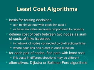
basis for routing decisions
basis for routing decisions
can minimize hop with each link cost 1
can minimize hop with each link cost 1
or have link value inversely proportional to capacity
or have link value inversely proportional to capacity
de
defines cost of path between two nodes as sum
fines cost of path between two nodes as sum
of costs of links traversed
of costs of links traversed
in network of nodes connected by bi-directional links
in network of nodes connected by bi-directional links
where e
where each link has a cost in each direction
ach link has a cost in each direction
for each pair of nodes, find path with least cost
for each pair of nodes, find path with least cost
link costs in different directions may be different
link costs in different directions may be different
alternatives:
alternatives: Dijkstra or Bellman-Ford algorithms
Dijkstra or Bellman-Ford algorithms
22.
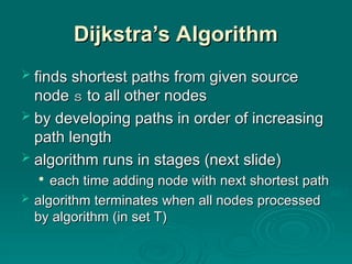
Dijkstra’s Algorithm
Dijkstra’s Algorithm
finds shortest paths from given source
finds shortest paths from given source
node
node s
s to all other nodes
to all other nodes
by developing paths in order of increasing
by developing paths in order of increasing
path length
path length
algorithm runs in stages (next slide)
algorithm runs in stages (next slide)
each time adding node with next shortest path
each time adding node with next shortest path
algorithm
algorithm terminates when all nodes processed
terminates when all nodes processed
by algorithm (in set T)
by algorithm (in set T)
23.
Dijkstra’s Algorithm Method
Dijkstra’sAlgorithm Method
Step 1
Step 1 [Initialization]
[Initialization]
T = {s}
T = {s} S
Set of nodes so far incorporated
et of nodes so far incorporated
L(n) = w(s, n) for n ≠ s
L(n) = w(s, n) for n ≠ s
initial
initial path costs to neighboring nodes are simply link costs
path costs to neighboring nodes are simply link costs
Step
Step 2
2 [Get Next Node]
[Get Next Node]
find neighboring node not in T
find neighboring node not in T with
with least-cost path from s
least-cost path from s
in
incorporate node into T
corporate node into T
also incorporate the edge that is incident on that node and a
also incorporate the edge that is incident on that node and a
node in T that contributes to the path
node in T that contributes to the path
Step
Step 3
3 [Update Least-Cost Paths]
[Update Least-Cost Paths]
L(n) = min[L(n), L(x) + w(x, n)]
L(n) = min[L(n), L(x) + w(x, n)] for all n
for all n
T
T
if latter term is minimum, path from s to n is path from s to x
if latter term is minimum, path from s to n is path from s to x
concatenated with edge from x to n
concatenated with edge from x to n
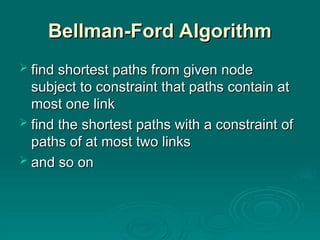
Bellman-Ford Algorithm
Bellman-Ford Algorithm
find shortest paths from given node
find shortest paths from given node
subject to constraint that paths contain at
subject to constraint that paths contain at
most one link
most one link
find
find the shortest paths with a constraint of
the shortest paths with a constraint of
paths of at most two links
paths of at most two links
and
and so on
so on
27.
Bellman-Ford Algorithm
Bellman-Ford Algorithm
step
step 1 [Initialization]
1 [Initialization]
L
L0
0(n) =
(n) =
, for all n
, for all n
s
s
L
Lh
h(s) = 0, for all h
(s) = 0, for all h
step
step 2 [Update]
2 [Update]
for each successive h
for each successive h
0
0
• for each n ≠ s, compute:
for each n ≠ s, compute: L
Lh+1
h+1(
(n
n)=
)=min
min
j
j[
[L
Lh
h(
(j
j)+
)+w
w(
(j,n
j,n)]
)]
connect n with predecessor node j that gives min
connect n with predecessor node j that gives min
eliminate
eliminate any connection of n with different
any connection of n with different
predecessor node formed during an earlier iteration
predecessor node formed during an earlier iteration
path
path from s to n terminates with link from j to n
from s to n terminates with link from j to n
Comparison
Comparison
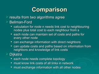
results fromtwo algorithms agree
results from two algorithms agree
Bellman-Ford
Bellman-Ford
calculation for node n needs link cost to neighbouring
calculation for node n needs link cost to neighbouring
nodes plus total cost to each neighbour from s
nodes plus total cost to each neighbour from s
each node can maintain set of costs and paths for
each node can maintain set of costs and paths for
every other node
every other node
can exchange information with direct neighbors
can exchange information with direct neighbors
can update costs and paths based on information from
can update costs and paths based on information from
neighbors and knowledge of link costs
neighbors and knowledge of link costs
Dijkstra
Dijkstra
each node needs complete topology
each node needs complete topology
must know link costs of all links in network
must know link costs of all links in network
must exchange information with all other nodes
must exchange information with all other nodes
31.
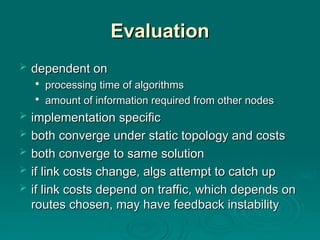
Evaluation
Evaluation
dependent on
dependenton
processing time of algorithms
processing time of algorithms
amount of information required from other nodes
amount of information required from other nodes
implementation specific
implementation specific
both converge under static topology and costs
both converge under static topology and costs
both converge to same solution
both converge to same solution
if link costs change, algs attempt to catch up
if link costs change, algs attempt to catch up
if link costs depend on traffic, which depends on
if link costs depend on traffic, which depends on
routes chosen, may have feedback instability
routes chosen, may have feedback instability
#1 Lecture slides prepared by Dr Lawrie Brown (UNSW@ADFA) for “Data and Computer Communications”, 8/e, by William Stallings, Chapter 12 “Routing in Switched Networks”.
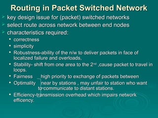
#2 A key design issue in switched networks, including packet-switching, frame relay, and ATM networks, and with internets, is that of routing. In general terms, the routing function seeks to design routes through the network for individual pairs of communicating end nodes such that the network is used efficiently. The primary function of a packet-switching network is to accept packets from a source station and deliver them to a destination station. To accomplish this, a path or route through the network must be determined; generally, more than one route is possible. Thus, a routing function must be performed. The requirements for this function are shown on the slide.
The first two items on the list, correctness and simplicity, are self-explanatory. Robustness has to do with the ability of the network to deliver packets via some route in the face of localized failures and overloads. The designer who seeks robustness must cope with the competing requirement for stability. Techniques that react to changing conditions have an unfortunate tendency to either react too slowly to events or to experience unstable swings from one extreme to another. A tradeoff also exists between fairness and optimality. Some performance criteria may give higher priority to the exchange of packets between nearby stations compared to an exchange between distant stations. This policy may maximize average throughput but will appear unfair to the station that primarily needs to communicate with distant stations. Finally, any routing technique involves some processing overhead at each node and often a transmission overhead as well, both of which impair network efficiency. The penalty of such overhead needs to be less than the benefit accrued based on some reasonable metric, such as increased robustness or fairness.
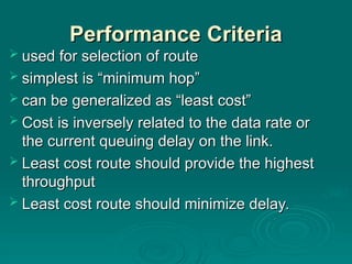
#3 The selection of a route is generally based on some performance criterion. The simplest criterion is to choose the minimum-hop route (one that passes through the least number of nodes) through the network. This is an easily measured criterion and should minimize the consumption of network resources. A generalization of the minimum-hop criterion is least-cost routing. In this case, a cost is associated with each link, and, for any pair of attached stations, the route through the network that accumulates the least cost is sought. In either the minimum-hop or least-cost approach, the algorithm for determining the optimum route for any pair of stations is relatively straightforward, and the processing time would be about the same for either computation. Because the least-cost criterion is more flexible, this is more common than the minimum-hop criterion. Several least-cost routing algorithms are in common use. These are described in Stallings DCC8e Section 12.3
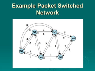
#4 Stallings DCC8e Figure 12.1 illustrates a network in which the two arrowed lines between a pair of nodes represent a link between these nodes, and the corresponding numbers represent the current link cost in each direction. The shortest path (fewest hops) from node 1 to node 6 is 1-3-6 (cost = 5 + 5 = 10), but the least-cost path is 1-4-5-6 (cost = 1 + 1 + 2 = 4). Costs are assigned to links to support one or more design objectives. For example, the cost could be inversely related to the data rate (i.e., the higher the data rate on a link, the lower the assigned cost of the link) or the current queuing delay on the link. In the first case, the least-cost route should provide the highest throughput. In the second case, the least-cost route should minimize delay.
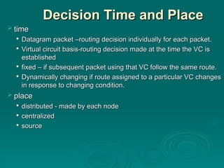
#5 Routing decisions are made on the basis of some performance criterion. Two key characteristics of the decision are the time and place that the decision is made.
Decision time is determined by whether the routing decision is made on a packet or virtual circuit basis. When the internal operation of the network is datagram, a routing decision is made individually for each packet. For internal virtual circuit operation, a routing decision is made at the time the virtual circuit is established. In the simplest case, all subsequent packets using that virtual circuit follow the same route. In more sophisticated network designs, the network may dynamically change the route assigned to a particular virtual circuit in response to changing conditions (e.g., overload or failure of a portion of the network).
The term decision place refers to which node or nodes in the network are responsible for the routing decision. Most common is distributed routing, in which each node has the responsibility of selecting an output link for routing packets as they arrive. For centralized routing, the decision is made by some designated node, such as a network control center. The danger of this latter approach is that the loss of the network control center may block operation of the network. The distributed approach is perhaps more complex but is also more robust. A third alternative, used in some networks, is source routing. In this case, the routing decision is actually made by the source station rather than by a network node and is then communicated to the network. This allows the user to dictate a route through the network that meets criteria local to that user.
#6 Routing decisions are made on the basis of some performance criterion. Two key characteristics of the decision are the time and place that the decision is made.
Decision time is determined by whether the routing decision is made on a packet or virtual circuit basis. When the internal operation of the network is datagram, a routing decision is made individually for each packet. For internal virtual circuit operation, a routing decision is made at the time the virtual circuit is established. In the simplest case, all subsequent packets using that virtual circuit follow the same route. In more sophisticated network designs, the network may dynamically change the route assigned to a particular virtual circuit in response to changing conditions (e.g., overload or failure of a portion of the network).
The term decision place refers to which node or nodes in the network are responsible for the routing decision. Most common is distributed routing, in which each node has the responsibility of selecting an output link for routing packets as they arrive. For centralized routing, the decision is made by some designated node, such as a network control center. The danger of this latter approach is that the loss of the network control center may block operation of the network. The distributed approach is perhaps more complex but is also more robust. A third alternative, used in some networks, is source routing. In this case, the routing decision is actually made by the source station rather than by a network node and is then communicated to the network. This allows the user to dictate a route through the network that meets criteria local to that user.
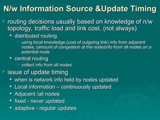
#7 Most routing strategies require that decisions be based on knowledge of the topology of the network, traffic load, and link cost.
With distributed routing, in which the routing decision is made by each node, the individual node may make use of only local information, such as the cost of each outgoing link. Each node might also collect information from adjacent (directly connected) nodes, such as the amount of congestion experienced at that node. Finally, there are algorithms in common use that allow the node to gain information from all nodes on any potential route of interest. In the case of centralized routing, the central node typically makes use of information obtained from all nodes.
A related concept is that of information update timing, which is a function of both the information source and the routing strategy. Clearly, if no information is used (as in flooding), there is no information to update. If only local information is used, the update is essentially continuous. For all other information source categories (adjacent nodes, all nodes), update timing depends on the routing strategy. For a fixed strategy, the information is never updated. For an adaptive strategy, information is updated from time to time to enable the routing decision to adapt to changing conditions.
As you might expect, the more information available, and the more frequently it is updated, the more likely the network is to make good routing decisions. On the other hand, the transmission of that information consumes network resources.
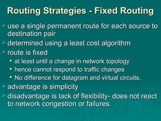
#8 A large number of routing strategies have evolved for dealing with the routing requirements of packet-switching networks, we survey four key strategies: fixed, flooding, random, and adaptive.
For fixed routing, a single, permanent route is configured for each source-destination pair of nodes in the network. Either of the least-cost routing algorithms described in Section 12.3 could be used. The routes are fixed, or at least only change when there is a change in the topology of the network. Thus, the link costs used in designing routes cannot be based on any dynamic variable such as traffic. They could, however, be based on expected traffic or capacity.
With fixed routing, there is no difference between routing for datagrams and virtual circuits. All packets from a given source to a given destination follow the same route. The advantage of fixed routing is its simplicity, and it should work well in a reliable network with a stable load. Its disadvantage is its lack of flexibility. It does not react to network congestion or failures.
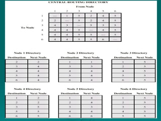
#9 Stallings DCC8e Figure 12.2 suggests how fixed routing might be implemented. A central routing matrix is created, to be stored perhaps at a network control center. The matrix shows, for each source-destination pair of nodes, the identity of the next node on the route. Note that it is not necessary to store the complete route for each possible pair of nodes. Rather, it is sufficient to know, for each pair of nodes, the identity of the first node on the route. To see this, suppose that the least-cost route from X to Y begins with the X-A link. Call the remainder of the route R1; this is the part from A to Y. Define R2 as the least-cost route from A to Y. Now, if the cost of R1 is greater than that of R2, then the X-Y route can be improved by using R2 instead. If the cost of R1 is less than R2, then R2 is not the least-cost route from A to Y. Therefore, R1 = R2. Thus, at each point along a route, it is only necessary to know the identity of the next node, not the entire route. In our example, the route from node 1 to node 6 begins by going through node 4. Again consulting the matrix, the route from node 4 to node 6 goes through node 5. Finally, the route from node 5 to node 6 is a direct link to node 6. Thus, the complete route from node 1 to node 6 is 1-4-5-6.
From this overall matrix, routing tables can be developed and stored at each node. From the reasoning in the preceding paragraph, it follows that each node need only store a single column of the routing directory. The node's directory shows the next node to take for each destination.
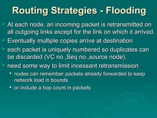
#10 Another simple routing technique is flooding. This technique requires no network information whatsoever and works as follows. A packet is sent by a source node to every one of its neighbors. At each node, an incoming packet is retransmitted on all outgoing links except for the link on which it arrived. Eventually, a number of copies of the packet will arrive at the destination. The packet must have some unique identifier (e.g., source node and sequence number, or virtual circuit number and sequence number) so that the destination knows to discard all but the first copy.
Unless something is done to stop the incessant retransmission of packets, the number of packets in circulation just from a single source packet grows without bound. One way to prevent this is for each node to remember the identity of those packets it has already retransmitted. When duplicate copies of the packet arrive, they are discarded. A simpler technique is to include a hop count field with each packet. The count can originally be set to some maximum value, such as the diameter (length of the longest minimum-hop path through the network) of the network. Each time a node passes on a packet, it decrements the count by one. When the count reaches zero, the packet is discarded.
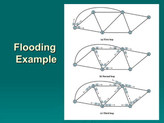
#11 An example of the latter tactic is shown in Stallings DCC8e Figure 12.3. The label on each packet in the figure indicates the current value of the hop count field in that packet. A packet is to be sent from node 1 to node 6 and is assigned a hop count of 3. On the first hop, three copies of the packet are created, and the hop count is decrement to 2. For the second hop of all these copies, a total of nine copies are created. One of these copies reaches node 6, which recognizes that it is the intended destination and does not retransmit. However, the other nodes generate a total of 22 new copies for their third and final hop. Each packet now has a hope count of 1. Note that if a node is not keeping track of packet identifier, it may generate multiple copies at this third stage. All packets received from the third hop are discarded, because the hop count is exhausted. In all, node 6 has received four additional copies of the packet.
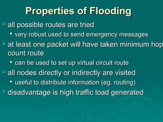
#12 The flooding technique has three remarkable properties:
• All possible routes between source and destination are tried. Thus, no matter what link or node outages have occurred, a packet will always get through if at least one path between source and destination exists.
• Because all routes are tried, at least one copy of the packet to arrive at the destination will have used a minimum-hop route.
• All nodes that are directly or indirectly connected to the source node are visited.
Because of the first property, the flooding technique is highly robust and could be used to send emergency messages. An example application is a military network that is subject to extensive damage. Because of the second property, flooding might be used initially to set up the route for a virtual circuit. The third property suggests that flooding can be useful for the dissemination of important information to all nodes; we will see that it is used in some schemes to disseminate routing information. The principal disadvantage of flooding is the high traffic load that it generates, which is directly proportional to the connectivity of the network.
#13 Random routing has the simplicity and robustness of flooding with far less traffic load. With random routing, a node selects only one outgoing path for retransmission of an incoming packet. The outgoing link is chosen at random, excluding the link on which the packet arrived. If all links are equally likely to be chosen, then a node may simply utilize outgoing links in a round-robin fashion.
A refinement of this technique is to assign a probability to each outgoing link and to select the link based on that probability. The probability could be based on data rate, or on fixed link costs.
Like flooding, random routing requires the use of no network information. Because the route taken is random, the actual route will typically not be the least-cost route nor the minimum-hop route. Thus, the network must carry a higher than optimum traffic load, although not nearly as high as for flooding.
#14 In virtually all packet-switching networks, some sort of adaptive routing technique is used. That is, the routing decisions that are made change as conditions on the network change. The principal conditions that influence routing decisions are:
• Failure: When a node or link fails, it can no longer be used as part of a route.
• Congestion: When a particular portion of the network is heavily congested, it is desirable to route packets around rather than through the area of congestion.
For adaptive routing to be possible, information about the state of the network must be exchanged among the nodes. There are several drawbacks associated with the use of adaptive routing, compared to fixed routing:
• The routing decision is more complex; therefore, the processing burden on network nodes increases.
• In most cases, adaptive strategies depend on status information that is collected at one place but used at another. There is a tradeoff here between the quality of the information and the amount of overhead. The more information that is exchanged, and the more frequently it is exchanged, the better will be the routing decisions that each node makes. On the other hand, this information is itself a load on the constituent networks, causing a performance degradation.
• An adaptive strategy may react too quickly, causing congestion-producing oscillation, or too slowly, being irrelevant.
#15 Despite these real dangers, adaptive routing strategies are by far the most prevalent, for two reasons:
• An adaptive routing strategy can improve performance, as seen by the network user.
• An adaptive routing strategy can aid in congestion control, which is discussed in Chapter 13. Because an adaptive routing strategy tends to balance loads, it can delay the onset of severe congestion.
These benefits may or may not be realized, depending on the soundness of the design and the nature of the load. By and large, adaptive routing is an extraordinarily complex task to perform properly. As demonstration of this, most major packet-switching networks, such as ARPANET and its successors, and many commercial networks, have endured at least one major overhaul of their routing strategy.
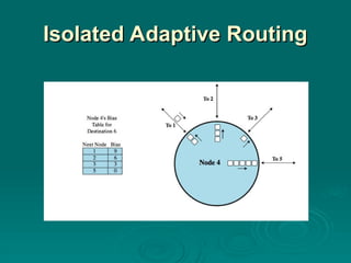
#16 A convenient way to classify adaptive routing strategies is on the basis of information source: local, adjacent nodes, all nodes. An example of an adaptive routing strategy that relies only on local information is one in which a node routes each packet to the outgoing link with the shortest queue length, Q. This would have the effect of balancing the load on outgoing links. However, some outgoing links may not be headed in the correct general direction. We can improve matters by also taking into account preferred direction, much as with random routing. In this case, each link emanating from the node would have a bias Bi, for each destination i, such that lower values of Bi indicate more preferred directions. For each incoming packet headed for node i, the node would choose the outgoing link that minimizes Q + Bi. Thus a node would tend to send packets in the right direction, with a concession made to current traffic delays.
Adaptive schemes based only on local information are rarely used because they do not exploit easily available information. Strategies based on information from adjacent nodes or all nodes are commonly found. Both take advantage of information that each node has about delays and outages that it experiences. Such adaptive strategies can be either distributed or centralized. In the distributed case, each node exchanges delay information with other nodes. Based on incoming information, a node tries to estimate the delay situation throughout the network, and applies a least-cost routing algorithm. In the centralized case, each node reports its link delay status to a central node, which designs routes based on this incoming information and sends the routing information back to the nodes.
#17 As an example, Stallings DCC8e Figure 12.4 show the status of node 4 of Figure 12.1 at a certain point in time. Node 4 has links to four other nodes. A fair number of packets have been arriving and a backlog has built up, with a queue of packets waiting for each of the outgoing links. A packet arrives from node 1 destined for node 6. To which outgoing link should the packet be routed? Based on current queue lengths and the values of bias (B6) for each outgoing link, the minimum value of Q + B6 is 4, on the link to node 3. Thus, node 4 routes the packet through node 3.
#18 In this section, we look at several examples of routing strategies. All of these were initially developed for ARPANET, which is a packet-switching network that was the foundation of the present-day Internet. It is instructive to examine these strategies.
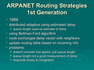
The original routing algorithm, designed in 1969, was a distributed adaptive algorithm using estimated delay as the performance criterion and a version of the Bellman-Ford algorithm. For this algorithm, each node maintains two vectors: Di = delay vector for node i, and Si = successor node vector for node i. Periodically (every 128 ms), each node exchanges its delay vector with all of its neighbors, which update both of their vectors using that info (see text for details). The estimated link delay is simply the queue length for that link. Thus, in building a new routing table, the node will tend to favor outgoing links with shorter queues. This tends to balance the load on outgoing links. However, because queue lengths vary rapidly with time, the distributed perception of the shortest route could change while a packet is en route. This could lead to a thrashing situation in which a packet continues to seek out areas of low congestion rather than aiming at the destination.
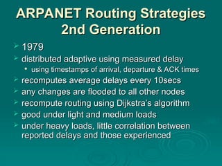
#19 After some years of experience and several minor modifications, the original routing algorithm was replaced by a quite different one in 1979. The new algorithm is also a distributed adaptive one, using delay as the performance criterion. Rather than using queue length as a surrogate for delay, the delay is measured directly. At a node, each incoming packet is timestamped with an arrival time. A departure time is recorded when the packet is transmitted. If a positive acknowledgment is returned, the delay for that packet is recorded as the departure time minus the arrival time plus transmission time and propagation delay. Every 10 seconds, the node computes the average delay on each outgoing link. If there are any significant changes in delay, the information is sent to all other nodes using flooding. Each node maintains an estimate of delay on every network link. When new information arrives, it recomputes its routing table using Dijkstra's algorithm. Experience with this new strategy indicated that it was more responsive and stable than the old one. The overhead induced by flooding was moderate because each node does this at most once every 10 seconds. However, as the load on the network grew, a shortcoming in the new strategy began to appear, due to the assumption that the measured packet delay on a link is a good predictor of the link delay encountered after all nodes reroute their traffic based on this reported delay. Thus, it is an effective routing mechanism only if there is some correlation between the reported values and those actually experienced after rerouting. This correlation tends to be rather high under light and moderate traffic loads. However, under heavy loads, there is little correlation. Therefore, immediately after all nodes have made routing updates, the routing tables are obsolete!
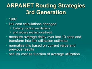
#20 The ARPANET designers concluded that the essence of the problem was that every node was trying to obtain the best route for all destinations, and that these efforts conflicted. It was concluded that under heavy loads, the goal of routing should be to give the average route a good path instead of attempting to give all routes the best path. The designers decided that it was unnecessary to change the overall routing algorithm. Rather, it was sufficient to change the function that calculates link costs, and this was revised in 1987. The calculation begins with measuring the average delay over the last 10 seconds. This value is then transformed with the following steps:
1. Using a simple single-server queuing model, the measured delay is transformed into an estimate of link utilization.
2. Result is smoothed by averaging it with previous estimate of utilization.
3. The link cost is then set as a function of average utilization that is designed to provide a reasonable estimate of cost while avoiding oscillation.
For the revised algorithm, the cost value is kept at the minimum value until a given level of utilization is reached. This feature has the effect of reducing routing overhead at low traffic levels. Above a certain level of utilization, the cost level is allowed to rise to a maximum value that is equal to three times the minimum value. The effect of this maximum value is to dictate that traffic should not be routed around a heavily utilized line by more than two additional hops. In summary, the revised cost function is keyed to utilization rather than delay. The function acts similar to a delay-based metric under light loads and to a capacity-based metric under heavy loads.
#21 Virtually all packet-switching networks and all internets base their routing decision on some form of least-cost criterion. If the criterion is to minimize the number of hops, each link has a value of 1. More typically, the link value is inversely proportional to the link capacity, proportional to the current load on the link, or some combination. In any case, these link or hop costs are used as input to a least-cost routing algorithm, which can be simply stated as:
“Given a network of nodes connected by bidirectional links, where each link has a cost associated with it in each direction, define the cost of a path between two nodes as the sum of the costs of the links traversed. For each pair of nodes, find a path with the least cost.”
Note that the cost of a link may differ in its two directions. This would be true, for example, if the cost of a link equaled the length of the queue of packets awaiting transmission from each of the two nodes on the link.
Most least-cost routing algorithms in use in packet-switching networks and internets are variations of one of two common algorithms, known as Dijkstra's algorithm and the Bellman-Ford algorithm. This section provides a summary of these two algorithms.
#22 Dijkstra's algorithm [DIJK59] can be stated as: Find the shortest paths from a given source node to all other nodes by developing the paths in order of increasing path length. The algorithm proceeds in stages. By the kth stage, the shortest paths to the k nodes closest to (least cost away from) the source node have been determined; these nodes are in a set T. At stage (k + 1), the node not in T that has the shortest path from the source node is added to T. As each node is added to T, its path from the source is defined.
#23 Dijkstra's Algorithm has three steps; steps 2 and 3 are repeated until T = N. That is, steps 2 and 3 are repeated until final paths have been assigned to all nodes in the network. Itcan be formally described as shown above, given the following definitions:
N = set of nodes in the network
s = source node
T = set of nodes so far incorporated by the algorithm
w(i, j) = link cost from node i to node j; w(i, i) = 0; w(i, j) = ∞ if two nodes not directly connected; w(i, j) ≥ 0 if two nodes are directly connected
L(n) = cost of the least-cost path from node s to node n that is currently known to the algorithm; at termination, this is the cost of the least-cost path in the graph from s to n.
The algorithm terminates when all nodes have been added to T. At termination, the value L(x) associated with each node x is the cost (length) of the least-cost path from s to x. In addition, T defines the least-cost path from s to each other node. One iteration of steps 2 and 3 adds one new node to T and defines the least-cost path from s to that node. That path passes only through nodes that are in T. To see this, consider the following line of reasoning. After k iterations, there are k nodes in T, and the least-cost path from s to each of these nodes has been defined. Now consider all possible paths from s to nodes not in T. Among those paths, there is one of least cost that passes exclusively through nodes in T (see Problem 12.4), ending with a direct link from some node in T to a node not in T. This node is added to T and the associated path is defined as the least-cost path for that node.
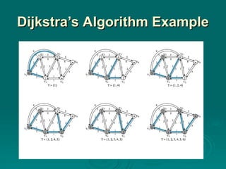
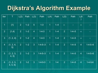
#24 Stallings DCC8e Table 12.2a (next slide) and Figure 12.9 show the result of applying this algorithm to the graph of Figure 12.1, using source node s = 1. The shaded edges define the spanning tree for the graph. The values in each circle are the current estimates of L(x) for each node x. A node is shaded when it is added to T. Note that at each step the path to each node plus the total cost of that path is generated. After the final iteration, the least-cost path to each node and the cost of that path have been developed. The same procedure can be used with node 2 as source node, and so on.
#25 Stallings DCC8e Table 12.2a shows the result of applying this algorithm as shown in Figure 12.9 (previous slide).
#26 The Bellman-Ford algorithm can be stated as: Find the shortest paths from a given source node subject to the constraint that the paths contain at most one link, then find the shortest paths with a constraint of paths of at most two links, and so on. This algorithm also proceeds in stages. The algorithm can be formally described as shown on the next slide, given the following definitions:
s = source node
w(i, j) = link cost from node i to node j
w(i, i) = 0
w(i, j) = if the two nodes are not directly connected
w(i, j) 0 if the two nodes are directly connected
h = maximum number of links in path at current stage of the algorithm
Lh(n) = cost of least-cost path from s to n under constraint of no more than h links
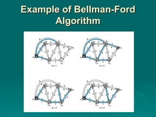
#27 The algorithm is formally described as shown. For the iteration of step 2 with h = K, and for each destination node n, the algorithm compares potential paths from s to n of length K + 1 with the path that existed at the end of the previous iteration. If the previous, shorter, path has less cost, then that path is retained. Otherwise a new path with length K + 1 is defined from s to n; this path consists of a path of length K from s to some node j, plus a direct hop from node j to node n. In this case, the path from s to j that is used is the K-hop path for j defined in the previous iteration.
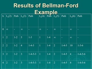
#28 Stallings DCC8e Table 12.2b(next slide) and Figure 12.10 show the result of applying this algorithm to Figure 12.1, using s = 1. At each step, the least-cost paths with a maximum number of links equal to h are found. After the final iteration, the least-cost path to each node and the cost of that path have been developed. The same procedure can be used with node 2 as source node, and so on. Note that the results agree with those obtained using Dijkstra's algorithm.
#29 Stallings DCC8e Table 12.2b and Figure 12.10 (previous slide) show the result of applying this algorithm to Figure 12.1, using s = 1. At each step, the least-cost paths with a maximum number of links equal to h are found. After the final iteration, the least-cost path to each node and the cost of that path have been developed. The same procedure can be used with node 2 as source node, and so on. Note that the results agree with those obtained using Dijkstra's algorithm.
#30 One interesting comparison can be made between these two algorithms, having to do with what information needs to be gathered. Consider first the Bellman-Ford algorithm. In step 2, the calculation for node n involves knowledge of the link cost to all neighboring nodes to node n ]i.e., w(j, n)] plus the total path cost to each of those neighboring nodes from a particular source node s [i.e., Lh(j)]. Each node can maintain a set of costs and associated paths for every other node in the network and exchange this information with its direct neighbors from time to time. Each node can therefore use the expression in step 2 of the Bellman-Ford algorithm, based only on information from its neighbors and knowledge of its link costs, to update its costs and paths.
On the other hand, consider Dijkstra's algorithm. Step 3 appears to require that each node must have complete topological information about the network. That is, each node must know the link costs of all links in the network. Thus, for this algorithm, information must be exchanged with all other nodes.
#31 In general, evaluation of the relative merits of the two algorithms should consider the processing time of the algorithms and the amount of information that must be collected from other nodes in the network or internet. The evaluation will depend on the implementation approach and the specific implementation.
A final point: Both algorithms are known to converge under static conditions of topology, and link costs and will converge to the same solution. If the link costs change over time, the algorithm will attempt to catch up with these changes. However, if the link cost depends on traffic, which in turn depends on the routes chosen, then a feedback condition exists, and instabilities may result.


![Dijkstra’s Algorithm Method
Dijkstra’s Algorithm Method
Step 1
Step 1 [Initialization]
[Initialization]
T = {s}
T = {s} S
Set of nodes so far incorporated
et of nodes so far incorporated
L(n) = w(s, n) for n ≠ s
L(n) = w(s, n) for n ≠ s
initial
initial path costs to neighboring nodes are simply link costs
path costs to neighboring nodes are simply link costs
Step
Step 2
2 [Get Next Node]
[Get Next Node]
find neighboring node not in T
find neighboring node not in T with
with least-cost path from s
least-cost path from s
in
incorporate node into T
corporate node into T
also incorporate the edge that is incident on that node and a
also incorporate the edge that is incident on that node and a
node in T that contributes to the path
node in T that contributes to the path
Step
Step 3
3 [Update Least-Cost Paths]
[Update Least-Cost Paths]
L(n) = min[L(n), L(x) + w(x, n)]
L(n) = min[L(n), L(x) + w(x, n)] for all n
for all n
T
T
if latter term is minimum, path from s to n is path from s to x
if latter term is minimum, path from s to n is path from s to x
concatenated with edge from x to n
concatenated with edge from x to n](https://image.slidesharecdn.com/186835548-12-routing-260202091843-cf282f70/85/Routing-in-packet-switching-and-circuit-ppt-23-320.jpg)
![Bellman-Ford Algorithm
Bellman-Ford Algorithm
step
step 1 [Initialization]
1 [Initialization]
L
L0
0(n) =
(n) =
, for all n
, for all n
s
s
L
Lh
h(s) = 0, for all h
(s) = 0, for all h
step
step 2 [Update]
2 [Update]
for each successive h
for each successive h
0
0
• for each n ≠ s, compute:
for each n ≠ s, compute: L
Lh+1
h+1(
(n
n)=
)=min
min
j
j[
[L
Lh
h(
(j
j)+
)+w
w(
(j,n
j,n)]
)]
connect n with predecessor node j that gives min
connect n with predecessor node j that gives min
eliminate
eliminate any connection of n with different
any connection of n with different
predecessor node formed during an earlier iteration
predecessor node formed during an earlier iteration
path
path from s to n terminates with link from j to n
from s to n terminates with link from j to n](https://image.slidesharecdn.com/186835548-12-routing-260202091843-cf282f70/85/Routing-in-packet-switching-and-circuit-ppt-27-320.jpg)