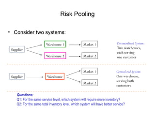
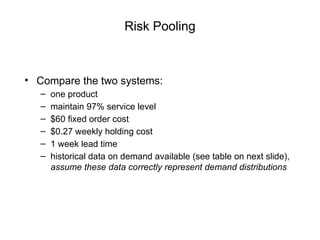
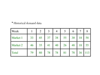
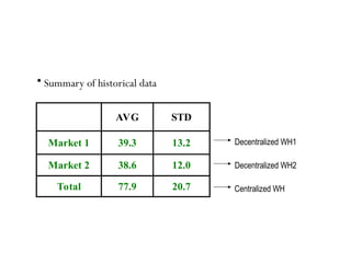
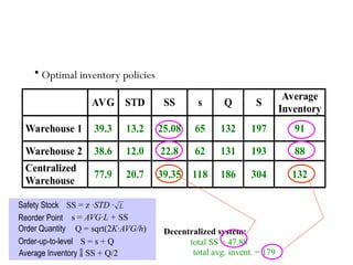
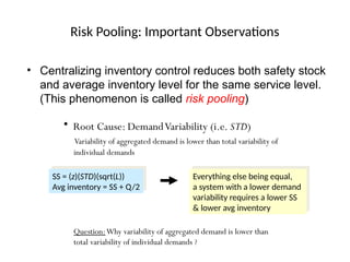
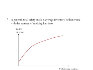
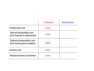
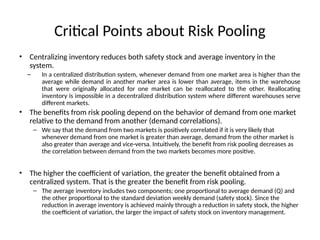
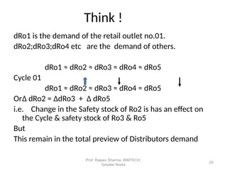
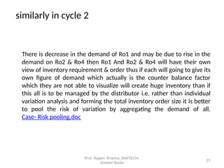
Risk Pooling
Risk Pooling
• Consider two systems:
Warehouse 1
Warehouse 2
Market 1
Market 2
Supplier
Decentralized System:
Two warehouses,
each serving
one customer
Warehouse
Market 1
Market 2
Supplier
Centralized System:
One warehouse,
serving both
customers
Questions:
Q1: For the same service level, which system will require more inventory?
Q2: For the same total inventory level, which system will have better service?
Risk Pooling
• Compare the two systems:
– one product
– maintain 97% service level
– $60 fixed order cost
– $0.27 weekly holding cost
– 1 week lead time
– historical data on demand available (see table on next slide),
assume these data correctly represent demand distributions
Risk Pooling Example
Week 1 2 3 4 5 6 7 8
Market 1 33 45 37 38 55 30 18 58
Market 2 46 35 41 40 26 48 18 55
Total 79 80 78 78 81 78 36 113
• Historical demand data
Risk Pooling Example
AVG STD
Market 1 39.3 13.2
Market 2 38.6 12.0
Total 77.9 20.7
• Summary of historical data
Decentralized WH1
Decentralized WH2
Centralized WH
Given n observations of a random variable, X1, X2, ..., Xn,
find mean, variance, and coefficient of variation
Mean
n
X
X
n
i
i


 1
Variance:
1
)
(
1
2
2





n
X
X
n
i
i

Standard deviation:
1
)
(
1
2





n
X
X
n
i
i

Coefficient of variation:
X
CV


Excel: Function AVERAGE()
Excel: Function STDEV()
Quick Review of Statistics
(s, S) Policy
Inventory
Level
S
s
0
Lead
Time
Lead
Time
Inventory Position
Q*
• Use EOQ model to determine optimal order quantity
– Q*
=
– Set S = Q* + s
×
2 K·AVG
h
Where
K = setup (ordering) cost
AVG = mean demand rate
h = unit holding cost per unit time
SS
More specifically….
• Model with uncertain demand, constant lead time
L = constant lead time
AVG = mean demand rate
STD = stdev of demand rate
Assume: Demand rate follows Normal(AVG, STD2
)
Reorder point: s = AVG · L + z · STD · L
Average demand
over lead time
Safety stock
Answer: Demand over lead time follows Normal(AVG·L, STD2
·L)
Question: what is the distribution of demand over lead time?
Risk Pooling Example
AVG STD SS s Q S
Average
Inventory
Warehouse 1 39.3 13.2 25.08 65 132 197 91
Warehouse 2 38.6 12.0 22.8 62 131 193 88
Centralized
Warehouse
77.9 20.7 39.35 118 186 304 132
• Optimal inventory policies
Decentralized system:
total SS = 47.88
total avg. invent. = 179
L
SS = z ·STD ·
s = AVG·L + SS
Q = sqrt(2K·AVG/h)
Safety Stock
Reorder Point
Order Quantity
Order-up-to-level S = s + Q
Average Inventory  SS + Q/2
Risk Pooling: Important Observations
• Centralizing inventory control reduces both safety stock
and average inventory level for the same service level.
(This phenomenon is called risk pooling)
• Root Cause: DemandVariability (i.e. STD)
Variability of aggregated demand is lower than total variability of
individual demands
SS = (z)(STD)(sqrt(L))
Avg inventory = SS + Q/2
Everything else being equal,
a system with a lower demand
variability requires a lower SS
& lower avg inventory
Question:Why variability of aggregated demand is lower than
total variability of individual demands ?
More Observations
• In general, total safety stock & average inventory both increase
with the number of stocking locations
Total SS
(Avg. Inv.)
# of stocking locations
Decentralized
Centralized
Inbound transportation cost
(from factories to warehouses)
Facility/Labor cost
Outbound transportation cost
(from warehouses to retailers)
Inventory cost
Responsiveness to customers
Lower
Lower
Higher
Lower
Lower
Centralized vs. Decentralized
Critical Points about Risk Pooling
• Centralizing inventory reduces both safety stock and average inventory in the
system.
– In a centralized distribution system, whenever demand from one market area is higher than the
average while demand in another marker area is lower than average, items in the warehouse
that were originally allocated for one market can be reallocated to the other. Reallocating
inventory is impossible in a decentralized distribution system where different warehouses serve
different markets.
• The benefits from risk pooling depend on the behavior of demand from one market
relative to the demand from another (demand correlations).
– We say that the demand from two markets is positively correlated if it is very likely that
whenever demand from one market is greater than average, demand from the other market is
also greater than average and vice-versa. Intuitively, the benefit from risk pooling decreases as
the correlation between demand from the two markets becomes more positive.
• The higher the coefficient of variation, the greater the benefit obtained from a
centralized system. That is the greater the benefit from risk pooling.
– The average inventory includes two components; one proportional to average demand (Q) and
the other proportional to the standard deviation weekly demand (safety stock). Since the
reduction in average inventory is achieved mainly through a reduction in safety stock, the higher
the coefficient of variation, the larger the impact of safety stock on inventory management.
• It is method to reduce stock keeping habit at
an individualistic levels.
• It is to pool the risk of the different players in
the chain ( But to an feasible extent)
Risk pooling
14
Prof. Rajeev Sharma, BIMTECH,
Greater Noida
How it works
Let’s assume some example:
Suppose there is a distributor of a specific product feeding the demand
of five retail outlets.
15
Prof. Rajeev Sharma, BIMTECH,
Greater Noida
Distributor
Retail
Outlet
01
Retail
out let
02
Retail
outlet 03
Retail
outlet 04
Retail
outlet 05
16
Prof. Rajeev Sharma, BIMTECH,
Greater Noida
Each outlet has the following inventory
IRo = CSi ( cycle stock to meet the average
demand) + SSi ( Safety Stock to meet any
variation in demand)
So based on its own experience each retailer
ascertain its own demand for the stock dRo
So total inventory size of the system is
= Sum ∑ (Iro1 +Iro2+Iro3+Iro4+Iro5+IroD)
17
Prof. Rajeev Sharma, BIMTECH,
Greater Noida
Think ! Inventory Size
18
Prof. Rajeev Sharma, BIMTECH,
Greater Noida
Now Let’s think different !
Why not to ask the distributor to meet the total demand of the system
and to take care of its variation. Rather summing up our total inventory
together with our individual experienced variation to be demanded
from the distributor.
i.e. ask him to take care of our entire inventory demand.
Or
to say pooling up our risk , of keeping separate inventory at each POS
to that at one POS.
i.e. replacing sum of variation of individual demand to
aggregate number of individual demand
19
Prof. Rajeev Sharma, BIMTECH,
Greater Noida
dRo1 is the demand of the retail outlet no.01.
dRo2;dRo3;dRo4 etc are the demand of others.
dRo1 ≈ dRo2 ≈ dRo3 ≈ dRo4 ≈ dRo5
Cycle 01
dRo1 ≈ dRo2 ≈ dRo3 ≈ dRo4 ≈ dRo5
OrΔ dRo2 = ΔdRo3 + Δ dRo5
i.e. Change in the Safety stock of Ro2 is has an effect on
the Cycle & safety stock of Ro3 & Ro5
But
This remain in the total preview of Distributors demand
Think !
20
Prof. Rajeev Sharma, BIMTECH,
Greater Noida
similarly in cycle 2
There is decrease in the demand of Ro1 and may be due to rise in the
demand on Ro2 & Ro4 then Ro1 And Ro2 & Ro4 will have their own
view of inventory requirement & order thus if each will going to give its
own figure of demand which actually is the counter balance factor
which they are not able to visualize will create huge inventory than if
this all is to be managed by the distributor i.e. rather than individual
variation analysis and forming the total inventory order size it is better
to pool the risk of variation by aggregating the demand of all.
Case- Risk pooling.doc
21
Prof. Rajeev Sharma, BIMTECH,
Greater Noida

Risk pooling FOR MBA STUDENTS OPERATIONS.pptx

  • 1.
  • 2.
    Risk Pooling • Considertwo systems: Warehouse 1 Warehouse 2 Market 1 Market 2 Supplier Decentralized System: Two warehouses, each serving one customer Warehouse Market 1 Market 2 Supplier Centralized System: One warehouse, serving both customers Questions: Q1: For the same service level, which system will require more inventory? Q2: For the same total inventory level, which system will have better service?
  • 3.
    Risk Pooling • Comparethe two systems: – one product – maintain 97% service level – $60 fixed order cost – $0.27 weekly holding cost – 1 week lead time – historical data on demand available (see table on next slide), assume these data correctly represent demand distributions
  • 4.
    Risk Pooling Example Week1 2 3 4 5 6 7 8 Market 1 33 45 37 38 55 30 18 58 Market 2 46 35 41 40 26 48 18 55 Total 79 80 78 78 81 78 36 113 • Historical demand data
  • 5.
    Risk Pooling Example AVGSTD Market 1 39.3 13.2 Market 2 38.6 12.0 Total 77.9 20.7 • Summary of historical data Decentralized WH1 Decentralized WH2 Centralized WH
  • 6.
    Given n observationsof a random variable, X1, X2, ..., Xn, find mean, variance, and coefficient of variation Mean n X X n i i    1 Variance: 1 ) ( 1 2 2      n X X n i i  Standard deviation: 1 ) ( 1 2      n X X n i i  Coefficient of variation: X CV   Excel: Function AVERAGE() Excel: Function STDEV() Quick Review of Statistics
  • 7.
    (s, S) Policy Inventory Level S s 0 Lead Time Lead Time InventoryPosition Q* • Use EOQ model to determine optimal order quantity – Q* = – Set S = Q* + s × 2 K·AVG h Where K = setup (ordering) cost AVG = mean demand rate h = unit holding cost per unit time SS
  • 8.
    More specifically…. • Modelwith uncertain demand, constant lead time L = constant lead time AVG = mean demand rate STD = stdev of demand rate Assume: Demand rate follows Normal(AVG, STD2 ) Reorder point: s = AVG · L + z · STD · L Average demand over lead time Safety stock Answer: Demand over lead time follows Normal(AVG·L, STD2 ·L) Question: what is the distribution of demand over lead time?
  • 9.
    Risk Pooling Example AVGSTD SS s Q S Average Inventory Warehouse 1 39.3 13.2 25.08 65 132 197 91 Warehouse 2 38.6 12.0 22.8 62 131 193 88 Centralized Warehouse 77.9 20.7 39.35 118 186 304 132 • Optimal inventory policies Decentralized system: total SS = 47.88 total avg. invent. = 179 L SS = z ·STD · s = AVG·L + SS Q = sqrt(2K·AVG/h) Safety Stock Reorder Point Order Quantity Order-up-to-level S = s + Q Average Inventory  SS + Q/2
  • 10.
    Risk Pooling: ImportantObservations • Centralizing inventory control reduces both safety stock and average inventory level for the same service level. (This phenomenon is called risk pooling) • Root Cause: DemandVariability (i.e. STD) Variability of aggregated demand is lower than total variability of individual demands SS = (z)(STD)(sqrt(L)) Avg inventory = SS + Q/2 Everything else being equal, a system with a lower demand variability requires a lower SS & lower avg inventory Question:Why variability of aggregated demand is lower than total variability of individual demands ?
  • 11.
    More Observations • Ingeneral, total safety stock & average inventory both increase with the number of stocking locations Total SS (Avg. Inv.) # of stocking locations
  • 12.
    Decentralized Centralized Inbound transportation cost (fromfactories to warehouses) Facility/Labor cost Outbound transportation cost (from warehouses to retailers) Inventory cost Responsiveness to customers Lower Lower Higher Lower Lower Centralized vs. Decentralized
  • 13.
    Critical Points aboutRisk Pooling • Centralizing inventory reduces both safety stock and average inventory in the system. – In a centralized distribution system, whenever demand from one market area is higher than the average while demand in another marker area is lower than average, items in the warehouse that were originally allocated for one market can be reallocated to the other. Reallocating inventory is impossible in a decentralized distribution system where different warehouses serve different markets. • The benefits from risk pooling depend on the behavior of demand from one market relative to the demand from another (demand correlations). – We say that the demand from two markets is positively correlated if it is very likely that whenever demand from one market is greater than average, demand from the other market is also greater than average and vice-versa. Intuitively, the benefit from risk pooling decreases as the correlation between demand from the two markets becomes more positive. • The higher the coefficient of variation, the greater the benefit obtained from a centralized system. That is the greater the benefit from risk pooling. – The average inventory includes two components; one proportional to average demand (Q) and the other proportional to the standard deviation weekly demand (safety stock). Since the reduction in average inventory is achieved mainly through a reduction in safety stock, the higher the coefficient of variation, the larger the impact of safety stock on inventory management.
  • 14.
    • It ismethod to reduce stock keeping habit at an individualistic levels. • It is to pool the risk of the different players in the chain ( But to an feasible extent) Risk pooling 14 Prof. Rajeev Sharma, BIMTECH, Greater Noida
  • 15.
    How it works Let’sassume some example: Suppose there is a distributor of a specific product feeding the demand of five retail outlets. 15 Prof. Rajeev Sharma, BIMTECH, Greater Noida
  • 16.
    Distributor Retail Outlet 01 Retail out let 02 Retail outlet 03 Retail outlet04 Retail outlet 05 16 Prof. Rajeev Sharma, BIMTECH, Greater Noida
  • 17.
    Each outlet hasthe following inventory IRo = CSi ( cycle stock to meet the average demand) + SSi ( Safety Stock to meet any variation in demand) So based on its own experience each retailer ascertain its own demand for the stock dRo So total inventory size of the system is = Sum ∑ (Iro1 +Iro2+Iro3+Iro4+Iro5+IroD) 17 Prof. Rajeev Sharma, BIMTECH, Greater Noida
  • 18.
    Think ! InventorySize 18 Prof. Rajeev Sharma, BIMTECH, Greater Noida
  • 19.
    Now Let’s thinkdifferent ! Why not to ask the distributor to meet the total demand of the system and to take care of its variation. Rather summing up our total inventory together with our individual experienced variation to be demanded from the distributor. i.e. ask him to take care of our entire inventory demand. Or to say pooling up our risk , of keeping separate inventory at each POS to that at one POS. i.e. replacing sum of variation of individual demand to aggregate number of individual demand 19 Prof. Rajeev Sharma, BIMTECH, Greater Noida
  • 20.
    dRo1 is thedemand of the retail outlet no.01. dRo2;dRo3;dRo4 etc are the demand of others. dRo1 ≈ dRo2 ≈ dRo3 ≈ dRo4 ≈ dRo5 Cycle 01 dRo1 ≈ dRo2 ≈ dRo3 ≈ dRo4 ≈ dRo5 OrΔ dRo2 = ΔdRo3 + Δ dRo5 i.e. Change in the Safety stock of Ro2 is has an effect on the Cycle & safety stock of Ro3 & Ro5 But This remain in the total preview of Distributors demand Think ! 20 Prof. Rajeev Sharma, BIMTECH, Greater Noida
  • 21.
    similarly in cycle2 There is decrease in the demand of Ro1 and may be due to rise in the demand on Ro2 & Ro4 then Ro1 And Ro2 & Ro4 will have their own view of inventory requirement & order thus if each will going to give its own figure of demand which actually is the counter balance factor which they are not able to visualize will create huge inventory than if this all is to be managed by the distributor i.e. rather than individual variation analysis and forming the total inventory order size it is better to pool the risk of variation by aggregating the demand of all. Case- Risk pooling.doc 21 Prof. Rajeev Sharma, BIMTECH, Greater Noida