1. Sound Source Localization
Under the supervision of Josef Str¨om Bartunek
by
Naga Kiran Machiraju (9503172570),
Shashidhar Sanda (9410108857)
June 19, 2016

2. Abstract
The aim of the project is to accurately estimate the location of sound source by using
signals received from the source by a linear array of microphones and using the concept
of Time Difference Of Arrival (TDOA)[1].The time delays are estimated using the Least
Mean Square algorithm(LMS)[2] with respect to reference microphone , then these rela-
tive delays which are calculated using the LMS algorithm are used in Steepest Descent
algorithm [2] for the estimation of location of the sound source.

3. Contents
1 Introduction 2
1.1 Problem Formulation . . . . . . . . . . . . . . . . . . . . . . . . . . . . . 2
2 Proposed Solution 3
3 Source Code 6
4 Results 8
5 Conclusions & Scope for Future Work 15
6 Appendices 16
6.1 Source code . . . . . . . . . . . . . . . . . . . . . . . . . . . . . . . . . . 16
6.2 Time-plan . . . . . . . . . . . . . . . . . . . . . . . . . . . . . . . . . . . 19
1

4. Chapter 1
Introduction
Localization of a sound source means to locate the sound source’s position as well as
the direction from where the sound arrives to the receiver.Sound is a form of energy which
uses particles of the medium to propagate,hence sound cannot travel vaccume though it
can propogate through soilds and fluids.It travels in the air at a speed of 343 meters/sec at
20°C[3],but sound takes some time to propagate through the medium,denser the medium
faster is its speed of propagation,if we know the speed of propagation of sound in the
medium which is present in between the source and the receiver and the delay in the
sound produced at source to the compared to the sound received at the receiver we can
calculate the distance between the sound source and the receiver. The estimate of the
source location can be improved if we use an array of microphones as the receiver provided
that both sound source and the recevier are stationary ,by using the concept of time delay
of arrival (TDOA)[1].
We use algorithms like Least Mean Square algorithm [2] and Steepest Descent al-
gorithm [2]. The adaptive filters are used here to estimate the delays between different
signals in terms of filter length . The location of the source is calculated using the gradient
of the squared error function in the estimated time delays.
1.1 Problem Formulation
A stationary sound source is to be localized based on the time delays in between
equiv distant microphones in a linear array which is located in a 2 dimensional Cartesian
coordinate system along the X-axis.
2

5. Chapter 2
Proposed Solution
Time Difference Of Arrival(TDOA)[1] is one of the many methods of localizing the
sound source.The method needs at least 4 microphones to localize the stationary source.
We assume a sound source to be located at (X,Y) and a linear array of microphones along
the X-axis of a 2 dimensional Cartesian coordinate system.
and
Figure 2.1: 2-D Cartesian coordinate system
Distance between the source and the microphones is calculated theoretically, then the
time delays with respect to the reference microphone are calculated(dti).
dti =
(x − id)2 + y2 − x2 + y2
C
seconds (2.1)
signal for the reference microphone is generated(x0), this signal is then used to get
the signals for the remaining N microphones(xi). Here i = 1, 2, 3, ... N.
3

6. Figure 2.2: Delaying the reference signal
Based on these delayed signals we estimate the error using Least Mean Square(LMS)
algorithm[2]
Wn+1 = Wn − µe(n)x∗
(n) (2.2)
x(n)——>reference signal
e(n)——>error and e(n) = d(n) - x(n)
d(n)——>desired signal
Wn——> weights of the filter
µ——>step size
4

7. Figure 2.3: Adaptive filter used for estimating the filter coefficients
Practically the delay is estimated using the slope of the phase(φ(ω)) of the weights of
the LMS filter[2]. The slope is estimated using the least square solution of the equation.
φ(ω) = mωn + c (2.3)
From the slope(m) we estimate the delays (Dti) based on the equation
DTi =
−(m + L)
2
samples (2.4)
Dti =
DTi
Fs
seconds (2.5)
From the estimated delays(Dti) and the theoretical delays(dti) calculated earlier we
calculate the error in the calculated of delay, using this error we calculate the squared
error function(G(x,y)).
G(x, y) = (
(x − id)2 + y2 − x2 + y2
C
− Dti)2
seconds (2.6)
We estimate the sound source location using the Steepest Descent algorithm[2] using
the gradient of the squared error function.
Wn+1 = Wn − µ ξ(n) (2.7)
ξ(n)——> squared error function
Wn——–> weights of the filter
n = 0, 1, 2, ... P - 1
P———->number of iterations
µ——–>step size
5

8. Chapter 3
Source Code
The problem solution is implemented in Matlab.The time delays at each microphone
with respect to the reference microphone are calculated by dividing the difference of
Euclidean distance between microphones,source and the Euclidean distance between ref-
erence microphone,source with speed of sound in air.The time delay calculation is imple-
mented in Matlab.The Matlab Function ”pdist(X,’euclidean’)” is used to calculate the
distance between two points.
for i=1:length(mics)
X=[source(1,1) source(1,2);mics(i,1) mics(i,2)];
mic source distance(i)=pdist(X,'euclidean');
mics delay time(i)=(mic source distance(i)-mic source distance(1))/c;
mics delay samples(i)=mics delay time(i)*fs;
end
The time delays are estimated in the above code is by using the analytical method.The
Time delays are also estimated using the Least Mean Square(LMS) Algorithm[2].To im-
plement LMS algorithm a random sound source signal is generated.The random sound
source signal arrives to each microphone at different time.The microphone signals with
delays are generated using the sinc filter and the filter function in the Matlab.The length
of the filter specifies how accurately a given system can be modeled by the adaptive fil-
ter.The filter length affects the convergence rate,by increasing or decreasing computation
time,it can affect the stability of the system, at certain step sizes, and it affects the min-
imum Mean Square Error(MSE).The filter length is choosen by trial and error process
and the effect of filter length can be seen in result section.
X0=randn(N,1);
filter length=400;
for i=1:N mics-1
w=sinc([-filter length/2:filter length/2]-mics delay samples(1,i+1));
Xdelayed(:,i)=filter(w,1,X0);
end
Least Mean Square(LMS) algorithm is implemented using the generated delayed micro-
phone signals.The delayed microphone signals are desired signals and the input to the
filter is the reference microphone signal.The filter weights are obtained in LMS algo-
rithm.The obtained filter weights are used in calculation of time delays.
6

9. w1=zeros(filter length,N mics-1);%initializing the filter coefficients to zero
mu=0.001; %step size
for i=filter length:N
X1=X0(i:-1:(i-filter length+1));
e=Xdelayed(i,:)-X1.'*w1; %error
w1=w1+mu*X1*e; %updating the filter coefficients
end
The time delays are estimated using the slope of phase of the filter coefficients ob-
tained in the LMS algorithm.The phase of filter is obtained using the filter weights.The
slope of phase of the filter is determined by least square solution.The estimated time
delays in samples is obtained by adding the slope with the delay the desired signal.The
estimated time delays are obtained in seconds by divided time delays with the sampling
frequency.The slope is determined in Matlab using the Matlab operator ’´.
w fft=fft(w1);%fft of filter coefficient for finding the phase of the filter
phase=unwrap(angle(w fft));%phase of the filter
p=0:(pi/filter length):(pi-(pi/filter length));%normalizing the phase
t=[p;ones(1,filter length)].';
for i=1:N mics-1;
phase slope=tphase(:,i);%slope of phase of filter
k(i,1)=phase slope(1,:);
T(i,1)=-((filter length/2)+k(i,1)./2);%Entire delays in samples
end
mics delay time1=T/fs;%Entire delays in seconds
To estimate the sound source location Steepest Descent Algorithm is implemented in
Matlab.The mean square error G(x,y) is minimized by steepest Descent algorithm which
approximates the source location.In this section symbolic variables are generated in order
to get the expression for getting the gradient.The initial source location values and the
step size is chosen and then iterate to get approximate sound source location.
syms x y %creating symbolic variables
G=0;dx=0;dy=0;
for i=1:N mics-1
G1(i)=(((sqrt((x-(i*d)).ˆ2 + (y).ˆ2) - sqrt((x).ˆ2 + (y).ˆ2)))
-(mics delay time1(i,1)*c)).ˆ2;
G=G+G1(i);
end
G2=matlabFunction(G);
xdiff=diff(G2,x);ydiff=diff(G2,y);
Fx=matlabFunction(xdiff);Fy=matlabFunction(ydiff);
initiate source=[1;1];%initiating the source location
mu1=0.1;%step size
estimated source(:,1)=initiate source-((mu1).*....
[Fx(initiate source(1,1),initiate source(2,1));....
Fy(initiate source(1,1),initiate source(2,1))]);
for i=2:5000
estimated source(:,i)=estimated source(:,i-1)-((mu1).*....
[Fx(estimated source(1,i-1),estimated source(2,i-1));.....
Fy(estimated source(1,i-1),estimated source(2,i-1))]);
end
disp(estimated source(:,i));%displaying the estimated source
7

10. Chapter 4
Results
In this project to locate the sound source we used the concept of TDOA[1].For carrying
out the procedure we assumed the following conditions.
ˆ Assumed a 2-D Cartesian coordinate system with sound source located at (8,6)
ˆ A linear array of 5 microphones is considered along x-axis with reference microphone
located at (0,0) and each microphone is separated by distance d=2 meters
ˆ sampling frequency is taken as 10000 Hz
ˆ speed of sound in air is 343 m/s
Based on the above assumptions the time delays of microphones with respect to
reference microphones are calculated analytically.
dt1 =
(8 − 1(2))2 + 62 −
√
82 + 62
343
= −0.0044seconds (4.1)
dt2 =
(8 − 2(2))2 + 62 −
√
82 + 62
343
= −0.0081seconds (4.2)
dt3 =
(8 − 3(2))2 + 62 −
√
82 + 62
343
= −0.0107seconds (4.3)
dt4 =
(8 − 4(2))2 + 62 −
√
82 + 62
343
= −0.0117seconds (4.4)
The analytically calculated time delays are
[-0.0044; -0.0081; -0.0107; -0.0117] seconds
The calculated time delays are negative because the reference microphone is taken at
origin.
8

11. Figure 4.1: Sinc Filter impulse response used for delaying the reference signal
Figure 4.2: Impulse response of LMS Filter weights estimated from the delayed signals
9

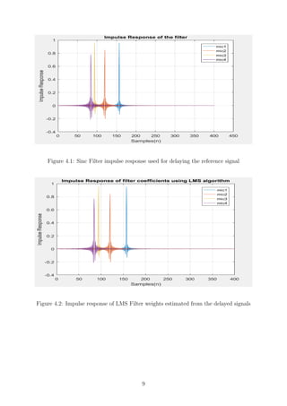
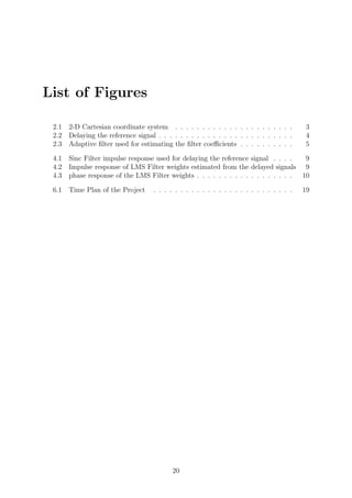
12. From the above two figures it is observed that the impulse response used for delaying
the signal and the impulse response of LMS Filter weights estimated from the delayed
signals are approximately same.
Figure 4.3: phase response of the LMS Filter weights
The phase response of the filter is approximately linear and the time delays are esti-
mated from the slope of the phase of the filter.
[-0.0044; -0.0081; -0.0107; -0.0119] seconds
10

13. The theoritically calculated time delays are matched with the estimated time delay using
the LMS algorithm.The results are tabled for different sound source location ,number of
microphones and the distance between each microphones.
source Number
of micro-
phones
Distance
between
micro-
phones
calculated Time
Delays
Estimated Time
Delays
Estimated
source
[8,6] 5 2 [0,-0.0044,-
0.0081,-0.0107,-
0.0117]
[0,-0.0044,-
0.0081,-0.0107,-
0.0119]
[8.0160,5.9469]
[10,5] 6 3 [0,-0.0075,-
0.0139,-0.117,-
0.0169]
[0,-0.0075,-
0.0139,-0.117,-
0.0169]
[10.016,5.048]
[12,8] 7 3 [0,-0.0069,-
0.0129,-0.0171,-
0.0187,-0.171,-
0.0129]
[0,-0.0072,-
0.0129,-0.0171,-
0.0187,-0.171,-
0.0129]
[11.993,8.004]
[5,3] 5 2 [0,-0.0046,-
0078,-0.0078,-
0.0046]
[0,-0.0049,-
0078,-0.0078,-
0.0049]
[5.042,3.006]
[9,3] 7 2.2 [0,-0.0060,-
0.0116,-
0.0165,-0.0189,-
0.0171,0.0126]
[0,-0.0060,-
0.0116,-
0.0164,-0.0189,-
0.0171,0.0126]
[9.000, 3.029]
[12.2,7.5]7 3.5 [0,-0.0083,-
0.0151,-0.0193,-
0.0193,-0.0150,-
0.0080]
[0,-0.0083,-
0.0151,-0.0193,-
0.0192,-0.0150,-
0.0083]
[12.298,7.639]
Table 4.1: Showing the calculated time delay and estimated time delay are approxmatly
equal
If Number of microphones increases to get better approximation of the sound source
location the distance between the microphones has to be decreased.The resultant source
location is tabulated by varying the distance between the microphones.
source Number of micro-
phones
Distance between micro-
phones
Estimated
source
[8,6] 3 5 [7.9561,5.8963]
[8,6] 4 4 [7.9698,5.8437]
[8,6] 5 3 [7.9863,5.9917]
[8,6] 6 2 [8.0192,6.0023]
Table 4.2: Shows that if Number of microphones increases to get better approximation
of the sound source the distance between the microphones has to be decreased.
11

14. By observing Table 4.2 to get the better estimation of source location the distance
between the microphones should be small.
The effect of sampling frequency over the estimated sound source location is observed and
tabulated.The sampling frequency is varied from the 1000Hz to 11000Hz,the resultant
sound source location is observed and tabulated.
Microphones=7;Source=(8,7);distance=2;filter length=200;stepsize=0.001;U=0.1
Sampling Frequency Estimated source
1000 [8.1819,6.1533]
3000 [8.0482,6.3288]
5000 [8.0738,6.9782]
7000 [7.9847,7.0341]
9000 [7.9907,7.0026]
9500 [8.0002,7.0104]
10000 [8.0468,7.3513]
11000 [8.1210,8.2065]
Table 4.3: The table shows the effect of change in the sampling frequency on estimated
source location
By observing Table 4.3 to get the better estimation of source the sampling frequency is
varied from 1000Hz to 11000Hz and at sampling frequency 9500Hz the estimated source
location is exactly near to the original source location.
The effect of change in the filter length on the estimated source location is observed
and tabulated.The filter length is varied from 200 to 1200 we get good approximation
of sound source till 600 and after 600 we get the results that are near to actual sound
source location.
Microphones=7;Source=(8,7);distance=2;stepsize=0.001;U=0.1
Filter Length Estimated source
200 (8.0512,7.3652)
250 (8.0095,7.0663)
300 (8.0041,6.9733)
400 (8.0041,6.9733)
500 (8.0041,6.9733)
600 (7.9827,6.8919)
900 (7.9628,6.7774)
1000 (7.9073,6.2424)
1100 (7.7924,6.0481)
1200 (7.7906,4.7082)
Table 4.4: The table shows the effect of change in the filter length on the estimated source
location
12

15. By observing Table 4.4 if the filter length of the system is increased, the number of
computations will increase, decreasing the maximum convergence rate.Conversely, if
the filter length is decreased, the number of computations will decrease, increasing the
maximum Convergence rate.By varying the filter length the effect on estimated source
location is observed.
As the number of iterations increases the better we get approximation.The iteration
number is varied and the resultant sound source location is observed and tabulated.
Microphones=7;Source=(8,7);distance=2;filter length=200;
stepsize=0.001;U=0.1;initial source=[1,1]
Number of Iterations Estimated source
100 (8.7631,9.3682)
200 (8.2547,7.781,)
300 (8.0601,7.1557)
500 (8.0041,6.9733)
1000 (8.0018,6.9660)
5000 (8.0018,6.9660)
10000 (8.0018,6.9660)
15000 (8.0018,6.9660)
Table 4.5: The table shows the effect of change in the Number of iterations on estimated
source location
By observing Table 4.5 the number of iterations increased from 100 to 15000 the effect
on estimated source location is seen.The iteration number is varied such that mean
square error reaches the steady state.For 1000 iterations the mean square error reaches
steady state so we get estimated source location near to original source location.
The effect of change in the stepsize used in steepest descent algorithm on the estimated
source location is tabulated.The resultant sound source location for different values of
stepsize is noted and tabulated.
Microphones=7;Source=(8,7);distance=2;filter length=200;
stepsize=0.001;initial source=[1,1]
Step Size(U) used in Steepest Descent al-
gorithm
Estimated source
0.05 (8.0018,6.9660)
0.01 (8.0017,9.655)
0.005 (7.9931,6.9373)
0.001 (7.6966,5.9494)
Table 4.6: The table shows the effect of change in the step size used in the steepest
descent algorithm on Estimated source location
13

16. The effect of change in the stepsize used in Least Mean Square algorithm on the estimated
source location is tabulated,if the stepsize decreases we get better approximation of
sound source location.The resultant sound source location for differnt values of stepsize
is noted and tabulated.
Microphones=7;Source=(8,7);distance=2;filter length=200;initial source=[1,1]
StepSize(µ) used in LMS algorithm Estimated source
0.01 (9.2453,1.4412)
0.01 (8.0018,6.9660)
0.0005 (7.9978,7.0945)
0.0001 (7.9978,7.0945)
0.00001 (7.9979,7.0947)
Table 4.7: The table shows the effect of change in the step size used in the LMS algorithm
on Estimated source location
If the step size is chosen small, the system will converge slowly, however,choosing a big
step size, the system will converge faster.
14

17. Chapter 5
Conclusions & Scope for Future
Work
The theoretically calculated delays are
[0,-0.0044,-0.0081,-0.0107,-0.0117] seconds
The delays estimated from the LMS filter weights are
[0,-0.0044,-0.0081,-0.0107,-0.0119] seconds
The Actual location of the sound source is (8, 6) meters and the location of the source
estimated finally is (8.0160, 5.9469) meters.
Hence stationary sound source has been localized in a 2 Dimensional environment to
a acceptable accuracy.
The effect of sampling frequency,filter length,number of iterations,step size in LMS al-
gorithm,step size in Steepest Descent algorithm over the estimated sound source location
is observed and tabulated.
This method can be further improved by using algorithms like Normalized Least
Mean Squares (NLMS) for more accurate delay estimations,by using an adaptive step
size in Steepest Descent Algorithm the source location can be estimated in lesser number
of iterations. This can be extended to locate a sound source in 3-D space with some
modifications . It can also be applied for locating a stationary source in real time.
Further it can be improvised to detect the moving source,tracking its position and many
applications that involve the acoustic sound source location.
15

18. Chapter 6
Appendices
6.1 Source code
%% clearing and closing commands
clc
clear all
close all
%% Assuming the source location,sampling frequency,number of microphones,
distance between each microphone
c=343;% speed of sound in air
fs=10000;%sampling frequncy
source=[8 6];%source location
N mics=5;% Number of microphones
d=2;% distance between each microphone
%% setting up Microphone positions
for i=0:N mics-1;
mics(i+1,:)=[d*i 0];
end
%% Estimating the time delay
for i=1:length(mics)
X=[source(1,1) source(1,2);mics(i,1) mics(i,2)];
mic source distance(i)=pdist(X,'euclidean');
%Time delay at each microphone in seconds
mics delay time(i)=(mic source distance(i)-mic source distance(1))/c;
%Time delay at each microphone in samples
mics delay samples(i)=mics delay time(i)*fs;
end
%% Delaying the signal using sinc and filter functions
N=10000;
X0=randn(N,1);% generating random point sound source signal
filter length=400;% filter length
figure;
for i=1:N mics-1
%sinc filter used for delaying the signal
w=sinc([-filter length/2:filter length/2]-mics delay samples(1,i+1));
Xdelayed(:,i)=filter(w,1,X0); % delayed signal
plot(w);
hold on
end
%% plotting impulse response of filter
16

19. grid on
hold off
title('Impulse Response of the filter');
xlabel('Samples(n)');
ylabel('Impulse Response');
legend('mic1','mic2','mic3','mic4')
%% Estimating the Time delay using the LMS algorithm
w1=zeros(filter length,N mics-1);
mu=0.001; %step size
for i=filter length:N
X1=X0(i:-1:(i-filter length+1));
e=Xdelayed(i,:)-X1.'*w1; %error
w1=w1+mu*X1*e; %updating the filter coefficients
end
%% plotting the Impulse Response of filter coefficients
obtained in LMS algorithm
figure;
plot(w1)
title('Impulse Response of filter coefficients using LMS algorithm');
xlabel('Samples(n)');
ylabel('Impulse Response');
legend('mic1','mic2','mic3','mic4')
grid on
%% Estimating the Time Delay in seconds and in samples
w fft=fft(w1);%fft of filter coefficient for finding the phase of the filter
phase=unwrap(angle(w fft));%phase of the filter
p=0:(pi/filter length):(pi-(pi/filter length));%normalizing the phase
t=[p;ones(1,filter length)].';
for i=1:N mics-1;
phase slope=tphase(:,i);%slope of phase of filter
k(i,1)=phase slope(1,:);
T(i,1)=-((filter length/2)+k(i,1)./2);%Entire delay in samples
end
mics delay time1=T/fs;%Entire delay in seconds
t1=p/pi;
%% plotting the phase response of the filter
figure;
plot(t1,phase)
title('Phase response of the filter');
xlabel('w/pi');
ylabel('Phase Response');
legend('mic1','mic2','mic3','mic4')
grid on
%% Source Localization using Steepest Descent algorithm
syms x y %creating symbolic variables
G=0;
dx=0;
dy=0;
for i=1:N mics-1
G1(i)=(((sqrt((x-(i*d)).ˆ2+(y).ˆ2)-.....
sqrt((x).ˆ2+(y).ˆ2)))-(mics delay time1(i,1)*c)).ˆ2;
G=G+G1(i);
end
G2=matlabFunction(G);
xdiff=diff(G2,x);
ydiff=diff(G2,y);
Fx=matlabFunction(xdiff);
Fy=matlabFunction(ydiff);
17

20. initiate source=[1;1];%initiating the source location
mu1=0.01;%step size
estimated source(:,1)=initiate source-.............
((mu1).*[Fx(initiate source(1,1),initiate source(2,1));....
Fy(initiate source(1,1),initiate source(2,1))]);
for i=2:5000
estimated source(:,i)=estimated source(:,i-1)-((mu1).*.....
[Fx(estimated source(1,i-1),estimated source(2,i-1));.....
Fy(estimated source(1,i-1),estimated source(2,i-1))]);
end
disp(estimated source(:,i));%displaying the estimated source
%% plotting the microphone location,source location
and estimated source location
figure;
plot(source(1,1),source(1,2),'*',mics(:,1),mics(:,2),'+')
axis([-5 20 -5 15])
hold on;
plot(estimated source(1,i),estimated source(2,i),'o')
title('2-D coordinate system')
legend('source location','mic location','Estimated source')
xlabel('X----->');
ylabel('Y----->');
grid on
%% plotting the Calculated Time delay and Estimated Time delay
mics delay time1=[0 mics delay time1.'];
y=0;
figure;
plot(mics delay time,y,'*')
hold on
plot(mics delay time1,y,'o')
title('Calculated time delay and Estimated time delay')
xlabel('X----->');
ylabel('Y----->');
legend('Calculated time delay','Estimated time delay')
grid on
18

21. 6.2 Time-plan
Figure 6.1: Time Plan of the Project
19

22. List of Figures
2.1 2-D Cartesian coordinate system . . . . . . . . . . . . . . . . . . . . . . 3
2.2 Delaying the reference signal . . . . . . . . . . . . . . . . . . . . . . . . . 4
2.3 Adaptive filter used for estimating the filter coefficients . . . . . . . . . . 5
4.1 Sinc Filter impulse response used for delaying the reference signal . . . . 9
4.2 Impulse response of LMS Filter weights estimated from the delayed signals 9
4.3 phase response of the LMS Filter weights . . . . . . . . . . . . . . . . . . 10
6.1 Time Plan of the Project . . . . . . . . . . . . . . . . . . . . . . . . . . 19
20

23. List of Tables
4.1 Showing the calculated time delay and estimated time delay are approx-
matly equal . . . . . . . . . . . . . . . . . . . . . . . . . . . . . . . . . . 11
4.2 Shows that if Number of microphones increases to get better approxima-
tion of the sound source the distance between the microphones has to be
decreased. . . . . . . . . . . . . . . . . . . . . . . . . . . . . . . . . . . . 11
4.3 The table shows the effect of change in the sampling frequency on estimated
source location . . . . . . . . . . . . . . . . . . . . . . . . . . . . . . . . 12
4.4 The table shows the effect of change in the filter length on the estimated
source location . . . . . . . . . . . . . . . . . . . . . . . . . . . . . . . . 12
4.5 The table shows the effect of change in the Number of iterations on esti-
mated source location . . . . . . . . . . . . . . . . . . . . . . . . . . . . . 13
4.6 The table shows the effect of change in the step size used in the steepest
descent algorithm on Estimated source location . . . . . . . . . . . . . . 13
4.7 The table shows the effect of change in the step size used in the LMS
algorithm on Estimated source location . . . . . . . . . . . . . . . . . . . 14
21

24. Bibliography
[1] Z. Chen, G. Gokeda, and Y. Yu. Introduction to Direction-of-Arrival Estima-
tion.Artech House signal processing library. Artech House, 2010.
[2] M.H. Hayes. Statistical digital signal processing and modeling. John Wiley &
Sons,1996
[3] A.J. Zuckerwar. Handbook of the Speed of Sound in Real Gases. Elsevier Science,
2002.
22