1. A Parallel Implementation of the Training of a
Backpropagation Multilayer Perceptron
Hlynur Davíð Hlynsson
Lisa Schmitz
May 2016
Abstract
This report presents an implementation and analysis of the node paral-
lelized training of a fully connected backpropagation multilayer perceptron.
The theoretical performance including speed up is calculated and compared
to measured experimental speed up.
1 Introduction
In the current days researchers were able to solve problems that have been labelled as
insolvable only a few years ago by applying machine learning algorithms. Computer vi-
sion and speech recognition are only two of many important application areas. Though
machine learning concepts like neural networks have been applied with great success
its complexity makes them a challenge for most computers. This report concentrates on
one machine learning concept which is the multilayer perceptron. Its computation time
will be improved by applying the node parallelization.
The training of a neural network with multiple layers is a computationally expensive
algorithm. Every node in the network requires the weighing and the summing of all
inputs in order to compute the activation function. This is later used to calculate the
error in every layer and update the weights accordingly. If a neural network is used in
context of image processing, game AI or general AI this can mean that these calculation
have to be made for millions of nodes. Fortunately many operations that are used to train
neural networks are heavily parallelizable and the training phase of those networks can
therefore be sped up immensely.
2 Multilayer Perceptron
A Multilayer Perceptron is a neural network that is commonly used in machine learning
e.g. pattern recognition or function approximation. In order to accomplish these tasks
it is trained with input data to produce a certain output. It consists of an input and an
output layer as well as one or more hidden layers in between as can be seen in figure 1.
1

2. Figure 1: Structure of a multilayer perceptron
The training of the network is supervised and consists of two different phases, the
forward and the backward pass.
In the forward pass the inputs are propagated through the network. Therefore the ac-
tivation of each node is computed by summing up the weighted inputs from the previous
layer and feeding the sum into a so called activation function. The activation function
that we chose is
φ(x) =
2
1 + exp(−x)
− 1
with the derivative
φ (x) =
(1 − φ(x))(1 + φ(x))
2
More formally, in the forward pass we compute the activations for each node n in
each layer l:
ol,n = φ
i
wl,n,iol−1,n
Where wl,n,i is the weight for input i to node n in layer l. The output of the network
are the values in layer L. Next we estimate the deltas for each node in the network,
which are the differences between the target outputs and the actual outputs:
δL,n = (oL,n − tn) · φ (φ−1
(oL,n))
= (oL,n − tn) ·
(1 + oL,n) · (1 − oL,n)
2
2

3. for the final layer l = L and
δl,n =
k
wl+1,k,nδl+1,k · φ (φ−1
(ol,n))
=
k
wl+1,k,nδl+1,k ·
(1 + ol,n) · (1 − ol,n)
2
for the other layers 2 = 1, . . . , L − 1.
Then the weights are updated:
wl,n,i = wl,n,i − η · ol,i · δl,n
with some good choice of learning rate η.
3 Parallelization strategy
The training algorithm of a multilayer perceptron offers possibilities for a variety of
parallelization strategies like training session parallelism, exemplar parallelism, weight
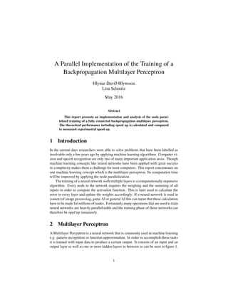
parallelism as well as node parallelism [1]. In this report the node parallelization strat-
egy has been implemented and analysed. In this parallelisaton strategy every processor
is responsible for a certain fraction of nodes per layer as can be seen in an example with
two processors in figure 2. This strategy benefits from networks with a high depth rather
than a large width.
Figure 2: Node parallelization with two processors
3

4. We use a linear data distribution to distribute the nodes that each processor is re-
sponsible for per layer. For layer l we define:
N(l) as the number of nodes in layer l
Kl =
N(l)
P
Rl = N(l) mod P
µl(n) = (p, i) where
p = max( n
K+1 , n−R
K
i = n − pK − min(p, R)
Ip,l =
N(l) + P + p − 1
P
µ−1
l (p, i) = pK + min(p, R) + i
After processor p has calculated the Ip,l values for his nodes in layer l, he broadcasts
them to the other processors so they can use them for calculations in layer l + 1 and so
on.
4 Implementation
This section presents pseudocode for the parallel implementation of each training phase.
The implementation of the forward and the backward pass is node parallelized.
4.1 Pseudocode for the forward phase
Here we generate the output of the network. Assume that W[l][n][i] is the weight
for input i to node n in layer l:
for l = 1:L
for j=1:I[p][l]
%Calculation phase
sum = 0
current = muInverse(p)(j)(l)
for i=1:N[l-1]
sum += W[l][current][i] * output[l-1][i]
end
output[l][current] = phi(sum)
%Communication phase
broadcast(output[l][muInverse(p)(j)(l)])
end
end
4

5. 4.2 Pseudocode for the backward phase
Now we determine the difference between targeted output values and the actual outputs
for each node:
for j=1:I[p][l]
%Calculation phase for final layer
current = muInverse(p)(j)(L)
o = output[L][current]
delta[L][current] = (mu(o) - t[j]) * ((1+o)*(1-o))*0.5
%Communication phase for final layer
broadcast(delta[L][muInverse(p)(j)(L)])
for l = L-1:1
for j=1:I[p][l]
%Calculation phase for the other layers
current = muInverse(p)(j)(l)
o = output[l][current]
sum = 0
for i=1:N[l+1]
sum = sum + W[l+1][i][current]*delta[l+1][i]
delta[l][j] = sum * ((1+o)*(1-o))*0.5
%Communication phase
broadcast(delta[l][muInverse(p)(j)(l)])
end
end
4.3 Weight update
Now we multiply the output delta with the input to get a gradient of the weight and
finally we update it.
for l = 1:L
for i=1:N[l-1]
%Calculation phase
current = muInverse(p)(i)(l)
W[l][current][i] -= eta * output[l-1][i] *
delta[l][current]
end
end
5 Typical problem run
In order to show that the implementation of the multilayer perceptron is correct a test im-
plementation has been made. In this implementation we train the multilayer perceptron
with a single input pattern. The weights of the network should be adjusted in a way that
5

6. the output gets close to the target values. The example we chose has the expected target
values [1.000000, −1.000000]. The output after the first epoch with random weights are
[0.494420, −0.322816]. But after 10000 epochs the weights have been adjusted so that
the output is now [0.953876, −0.953714] which - after thresholding - results in exactly
the expected target values.
6 Theoretical performance estimation
Performance estimations have been made for each phase and for the complete training
process.
6.1 Estimations of each phase
This part of the report gives a performance estimation for the forward, the backward
and the weight update phase of the training.
6.1.1 Forward pass
For a sequential program, the running time is
tcomp, 1 = ta ·
L−1
l=1
N(l) · N(l − 1)
for multiplying weights with inputs for each node and
tcomp, 2 = ta ·
L−1
l=1
N(l)
for passing the sums to the transfer function, amounting to
T1 = tcomp, 1 + tcomp, 2 = ta ·
L−1
l=1
N(l) · N(l − 1) + ta ·
L−1
l=1
N(l)
The parallel calculation time is
tcomp = ta ·
L−1
l=1
N(l − 1)Ip,l + ta ·
L−1
l=1
Ip,l
and communication, assuming that a broadcast operation is approximately log(P):
tcomm ≈ (tstartup + tdata) · log(P) ·
L−1
l=1
N(l)
So the parallel running time is
TP = tcomp + tcomm
6

7. = ta ·
L−1
l=1
N(l − 1)Ip,l + ta ·
L−1
l=1
Ip,l + (tstartup + tdata) · log(P) ·
L−1
l=1
N(l)
and we estimate the speedup, assuming that N(l) = n for all l:
SP =
T∗
S
TP
=
ta · (L − 1) · n2
+ ta · (L − 1) · n
ta · (L − 1) · n · Ip,l + ta · (L − 1) · Ip,l + (tstartup + tdata) · log(P) · (L − 1) · n
=
ta · n2
+ ta · n
ta · n · n
P + ta · n
P + (tstartup + tdata) · log(P) · n
= P ·
(n + 1)
(n + 1) + P ·
tstartup+tdata
ta
· log(P)
So we can expect a roughly linear speedup in this case for low values of P compared to
n.
6.1.2 Backward pass
In the sequential version of the backward pass we have to perform 3 subtractions/addi-
tions and 3 muliplications for each node in the final layer:
tcomp, 1 = t1 · 9 · L
and multiply together the delta with the output for each node and then add all these
terms together for each layer:
tcomp, 2 = ta ·
L−1
l=1
N(l) + N(l + 1)
for making the sequential running time
T∗
S = tcomp, 1 + tcomp, 2 = ta · 9 · L + ta ·
L−1
l=1
N(l) · N(l + 1)
The parallel calculation time is
tcomp = ta · 9 · Ip,L + ta ·
L−1
l=1
Ip,l · N(l + 1)
and communication with the same assumption as above:
tcomm ≈ (tstartup + tdata) · log(P) ·
L−1
l=1
N(l)
So the parallel running time is
7

8. TP = tcomp + tcomm
= ta · 9 · Ip,L + ta ·
L−1
l=1
Ip,l · N(l + 1) + (tstartup + tdata) · log(P) ·
L−1
l=1
N(l)
and we estimate the speedup under the same circumstances as above:
SP =
T∗
S
TP
=
ta · 9 · L + ta · (L − 1) · n2
ta · 9 · n
P + ta · (L − 1) · n
P · n + (tstartup + tdata) · log(P) · (L − 1) · n
= P ·
9 · L
n·(L−1) + n
9
L−1 + n +
(tstartup+tdata)
ta
· log(P) · P
Which is again roughly linear for low values of P compared to n.
6.2 Aggregate estimation
Thus we get the estimated speedup for a whole sequence of forward pass, backward
pass and weight update:
SP =
T∗
S
TP
= P ·
2n + 2 + 9 · L
n·(L−1)
2n + 2 + 2P ·
tstartup+tdata
ta
· log(P) + 9
L−1
By fixing L = 7 and assuming tstartup = tdata = ta = 1 we tabulate the speedup as a
function of P, first for n = 132 then n = 32000:
Processors Speedup n = 132 speedup n = 32k
1 1.02 1.00
2 2.01 2.00
4 3.79 4.00
8 6.58 7.99
16 9.88 15.95
Table 1: Theoretical speedup
8

9. 7 Experimental speedup
First we isolated the effect of only the forward pass and measured the speedup using
The PDC Center for High Performance Computing, see table 2. In these experiments,
we had a network with the depth of 7 layers, input with dimension 132 and and a width
of 64,000 nodes in every subsequent layer.
Processors PDC time in seconds
1 1.00
2 2.78
4 5.49
8 10.40
16 15.72
Table 2: Forward pass speedup
Then we did the same with the backward pass as well, see table 3.
Processors Speedup in seconds
1 1.00
2 1.98
4 3.92
8 7.07
16 9.95
Table 3: Forward pass speedup
8 Conclusion
The parallel implementation of the training algorithm of a multilayer perceptron pre-
sented in this paper lead to an almost linear speed up in both theory and experiments.
Choosing node parallelization as the main strategy illustrates the possible speed up of
this training algorithm. Nevertheless, this is only one way of parallelization and pa-
pers mention for example parallelization over each input pattern the network is trained
with. This could be a way to achieve an even better speed up. Since the focus in this
experiment lies on the speed up of one batch training phase the achieved speed up is
satisfying.
9

10. References
[1] M. Pethick, M. Liddle, P. Werstein, and Z. Huang, “Parallelization of a backprop-
agation neural network on a cluster computer,” in International conference on par-
allel and distributed computing and systems (PDCS 2003), 2003.
10