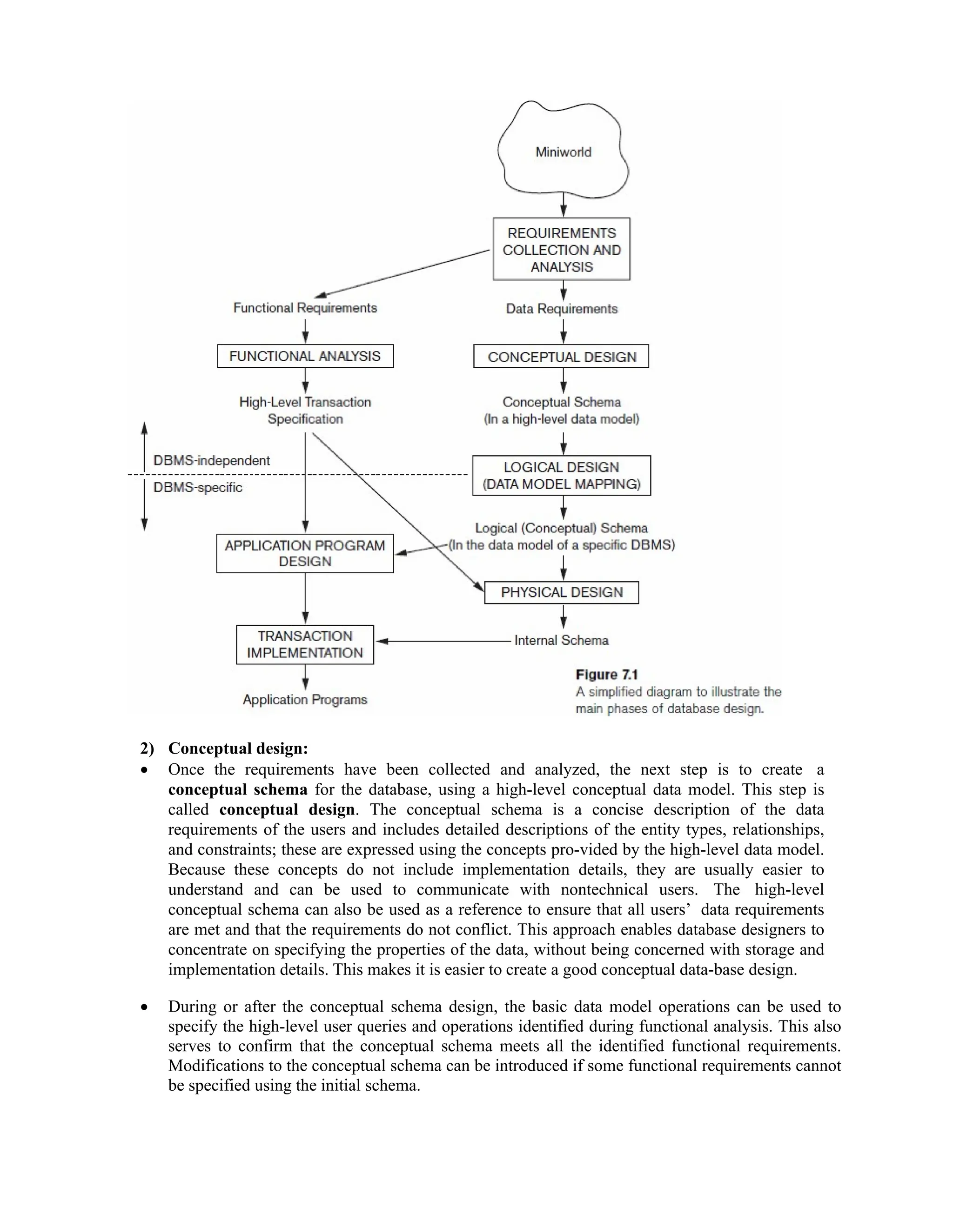
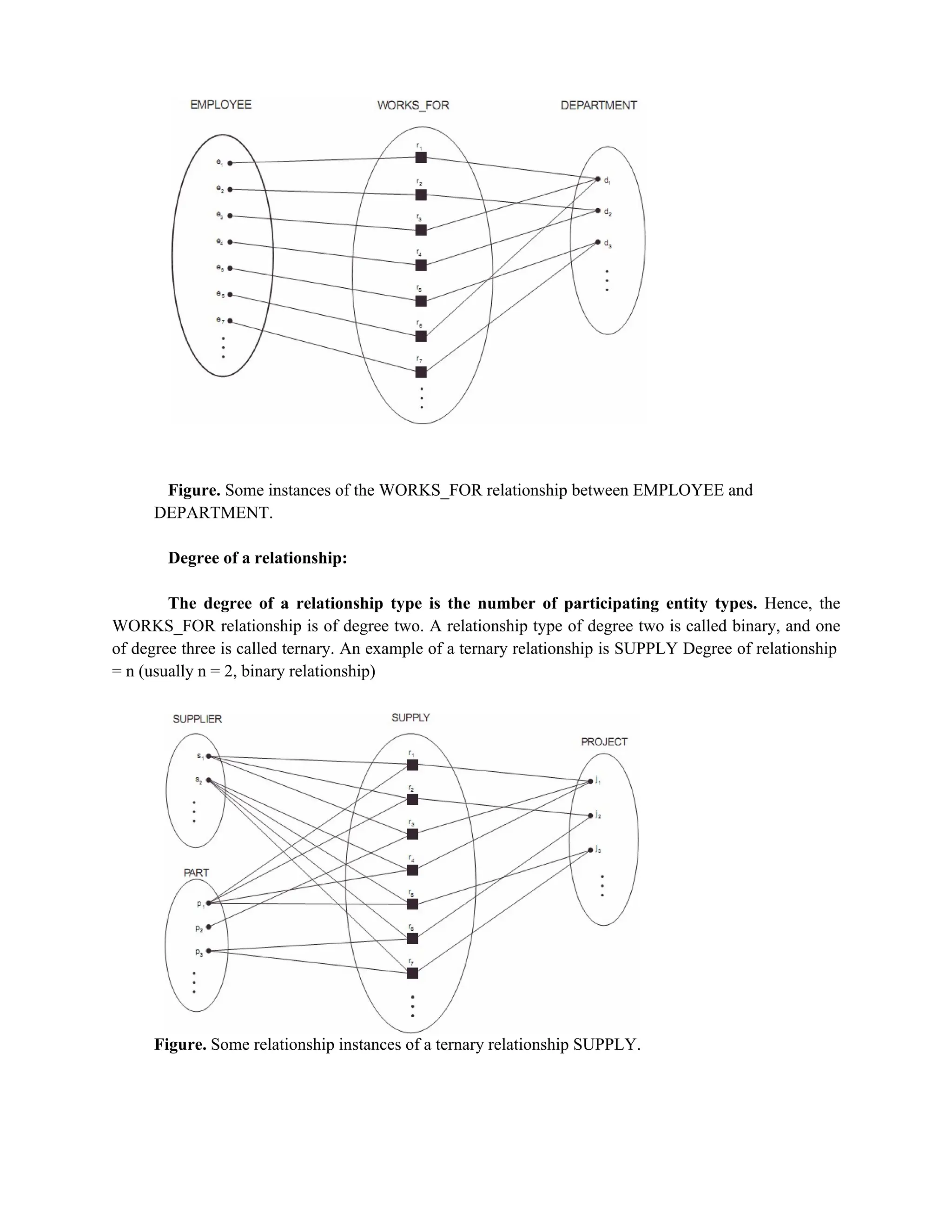
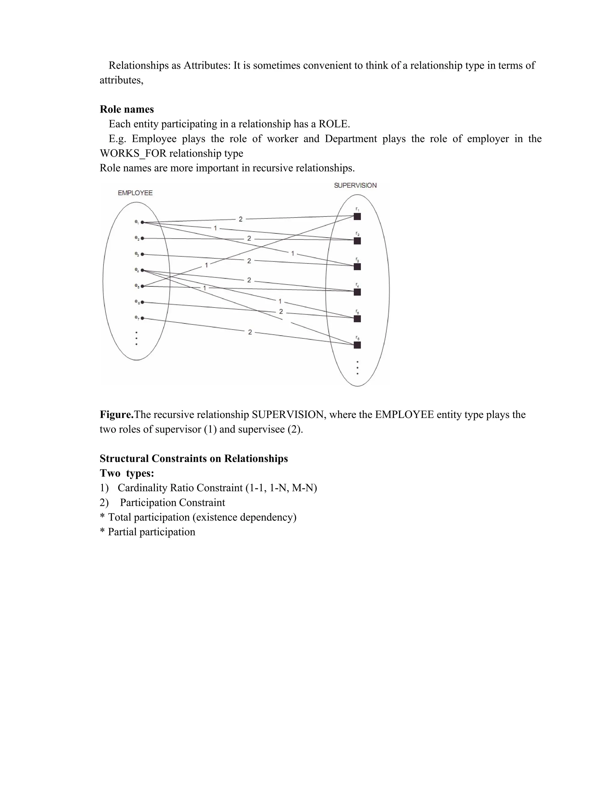
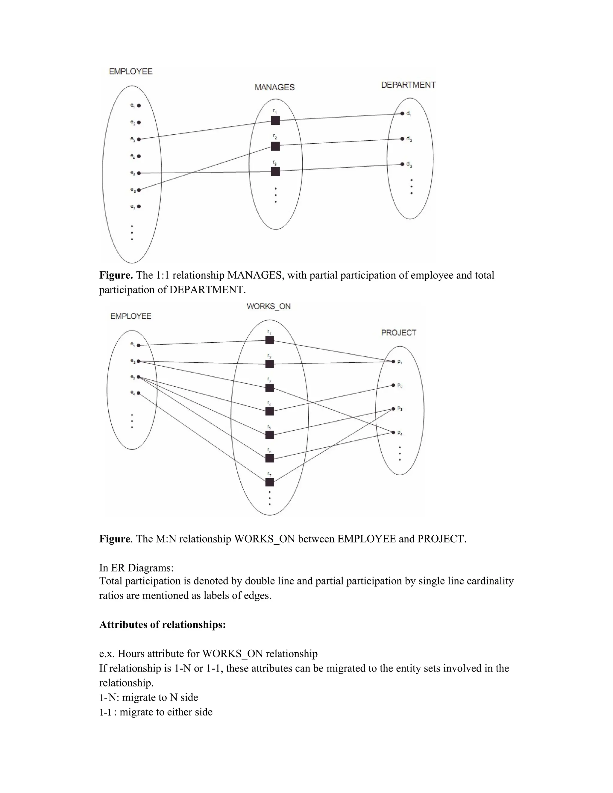
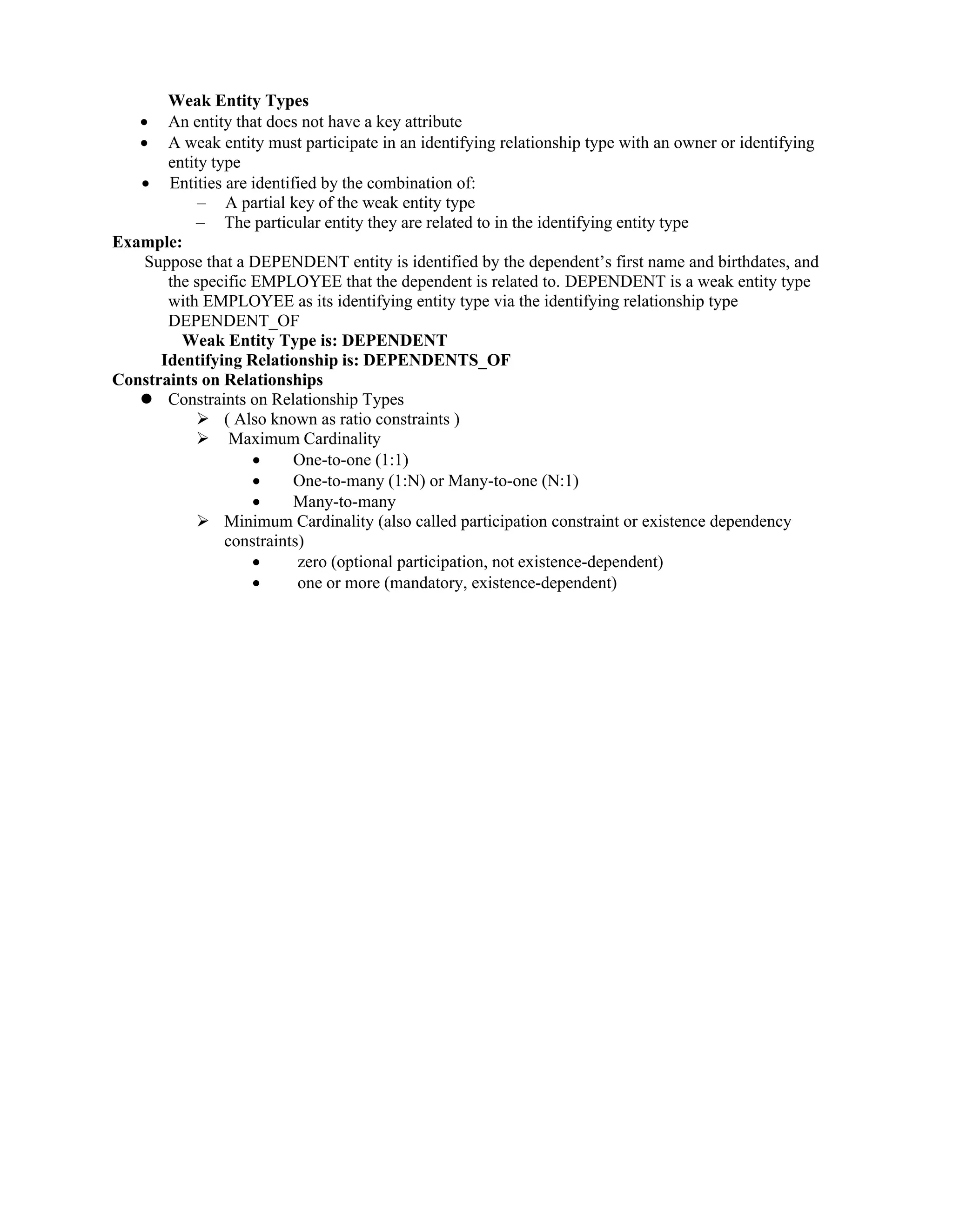
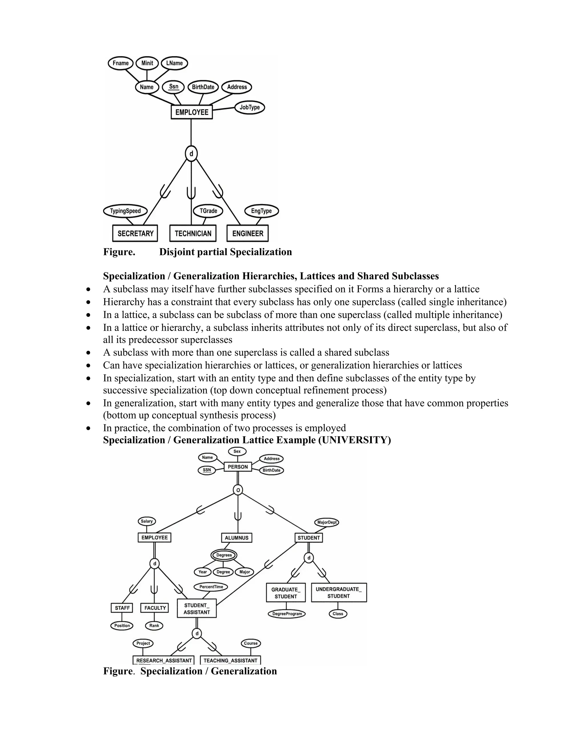
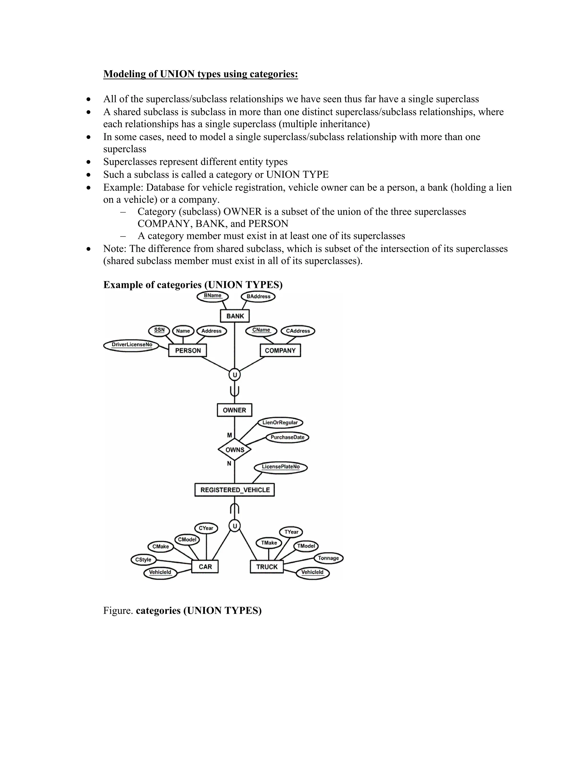
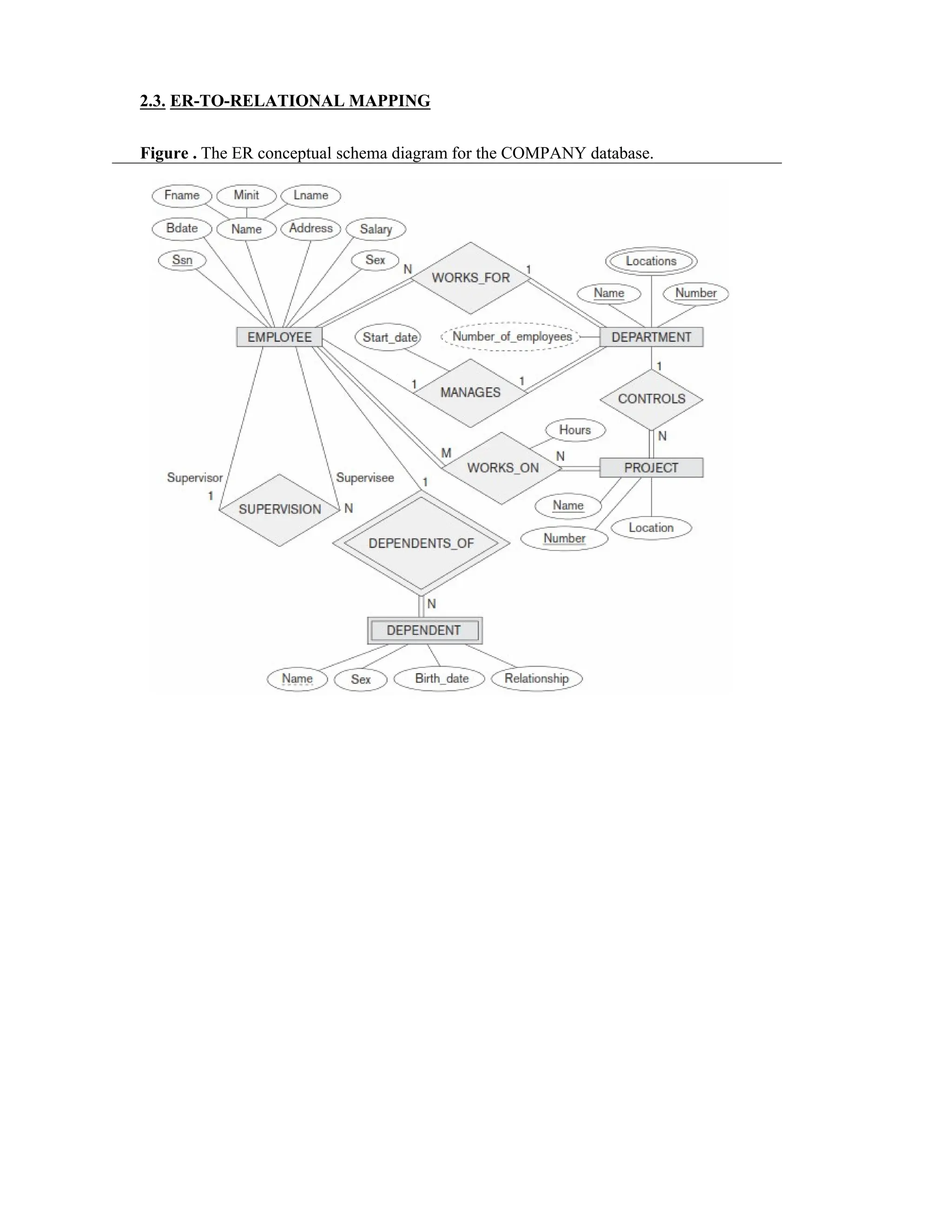
The document outlines the process of database design using the entity-relationship (ER) model, emphasizing requirements analysis, conceptual design, logical design, and physical design stages. It discusses the classification of data elements into entities, attributes, and relationships, detailing various types of attributes such as composite, multivalued, stored, and derived attributes. An example of a company database application is provided to illustrate these concepts and their representation in ER diagrams.

![Step 6: Mapping of Multivalued Attributes:
For each multivalued attribute A, create a new relation R. This relation R will include an attribute
corresponding to A, plus the primary key attribute K—as a foreign key in R—of the relation that repre-
sents the entity type or relationship type that has A as a multivalued attribute. The primary key of R is the
combination of A and K. If the multivalued attribute is com-posite, we include its simple components.
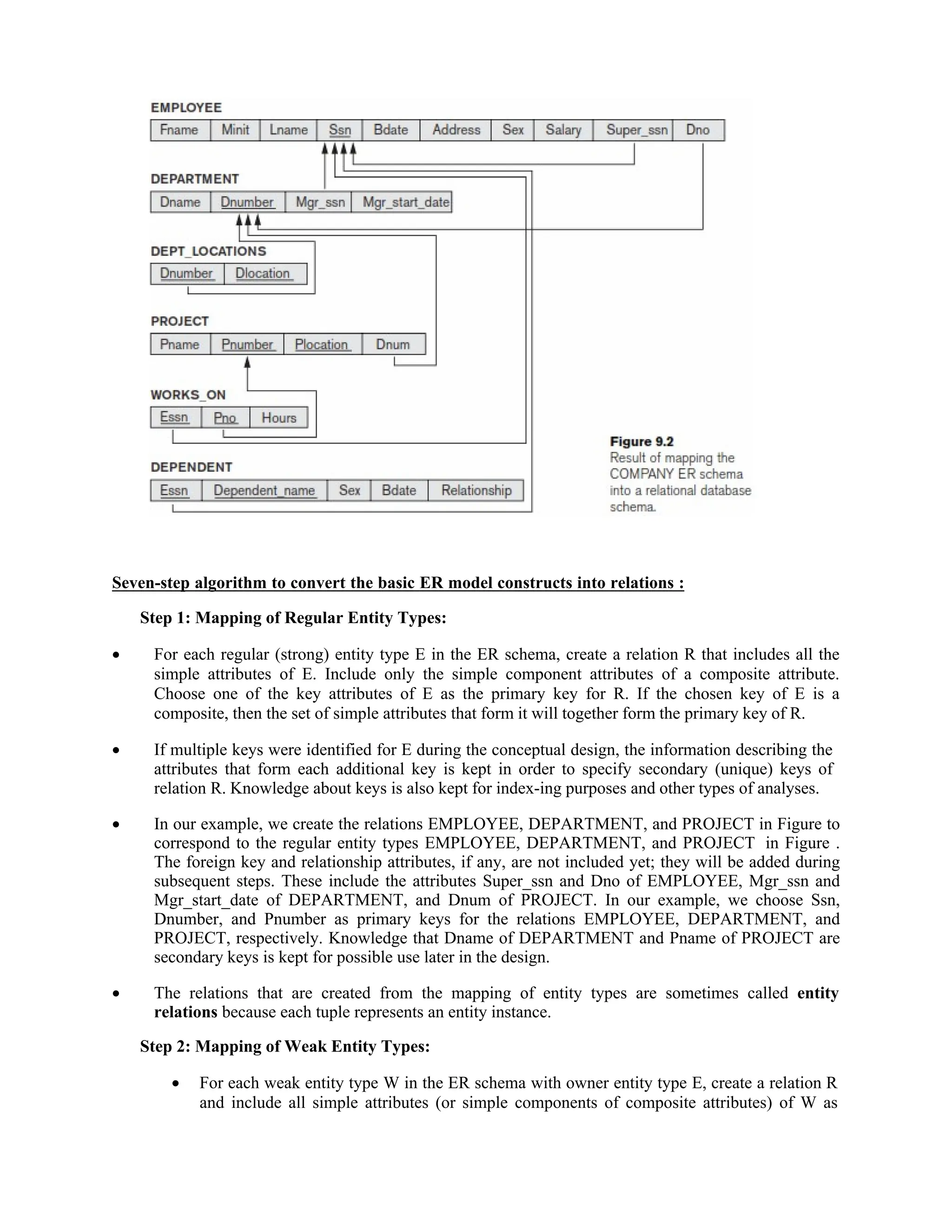
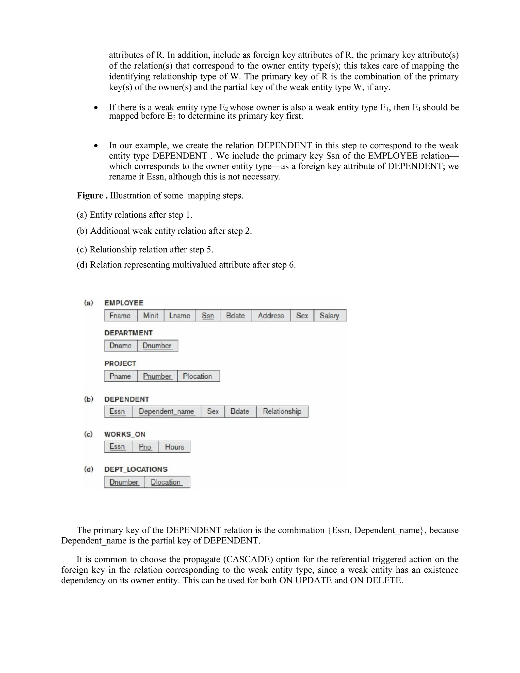
In our example, we create a relation DEPT_LOCATIONS (see Figure 9.3(d)). The attribute Dlocation
represents the multivalued attribute LOCATIONS of DEPARTMENT, while Dnumber—as foreign
key—represents the primary key of the DEPARTMENT relation. The primary key of
DEPT_LOCATIONS is the combination of {Dnumber, Dlocation}. A separate tuple will exist in
DEPT_LOCATIONS for each loca-tion that a department has.
The propagate (CASCADE) option for the referential triggered action should be specified on the
foreign key in the relation R corresponding to the multivalued attribute for both ON UPDATE and ON
DELETE. We should also note that the key of R when mapping a composite, multivalued attribute
requires some analysis of the meaning of the component attributes. In some cases, when a multi-valued
attribute is composite, only some of the component attributes are required to be part of the key of R; these
attributes are similar to a partial key of a weak entity type that corresponds to the multivalued attribute .
Step 7: Mapping of N-ary Relationship Types:
For each n-ary relationship type R, where n > 2, create a new relation S to represent R. Include as
foreign key attributes in S the primary keys of the relations that represent the participating entity types.
Also include any simple attributes of the n-ary relationship type (or simple components of composite
attributes) as attributes of S. The primary key of S is usually a combination of all the foreign keys that
reference the relations representing the participating entity types. However, if the cardinality constraints
on any of the entity types E participating in R is 1, then the primary key of S should not include the
foreign key attribute that references the relation E corresponding to E.
Table . Correspondence between ER and Relational Models
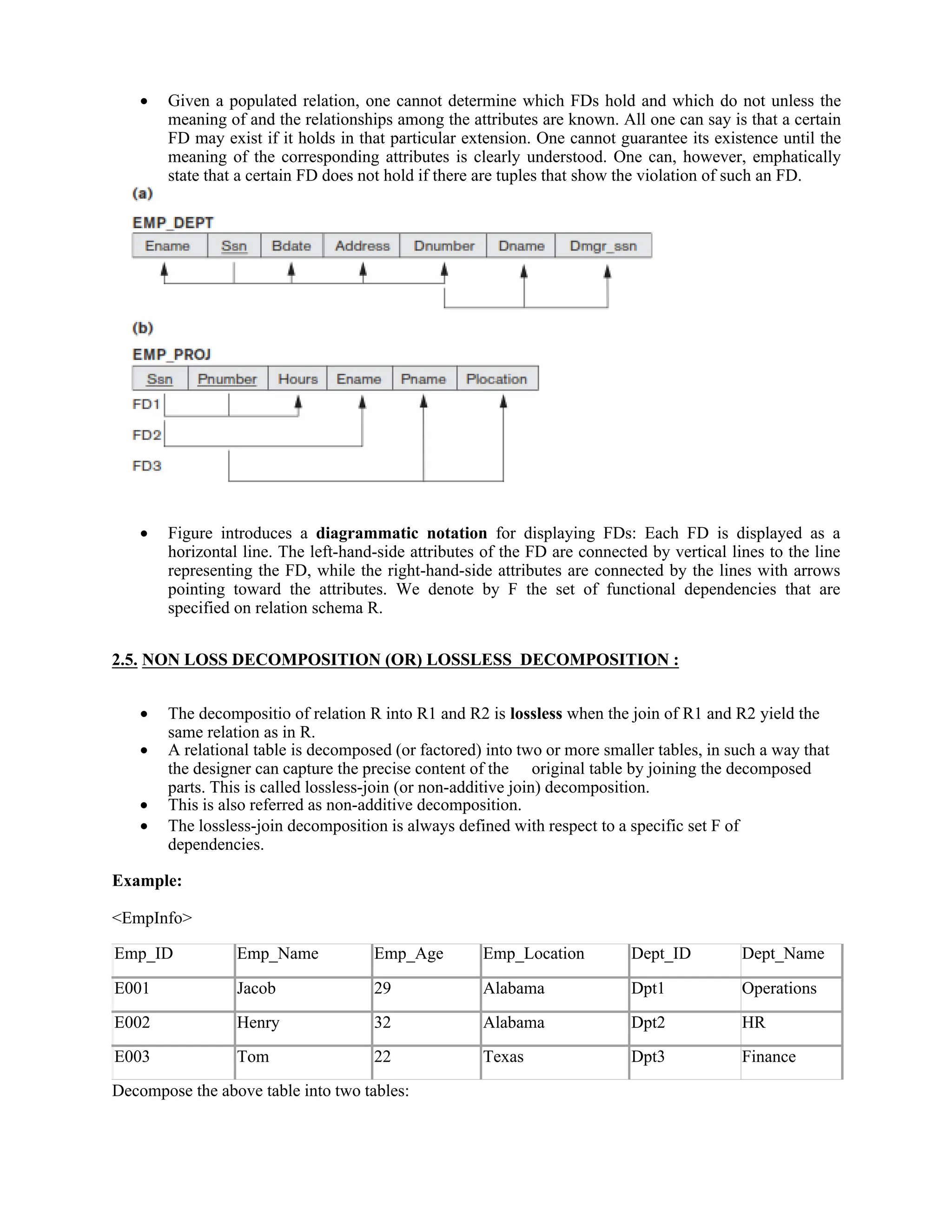
2.4. FUNCTIONAL DEPENDENCIES:
A functional dependency is a constraint between two sets of attributes from the database.
A functional dependency, denoted by X → Y, between two sets of attributes X and Y that are
subsets of R specifies a constraint on the possible tuples that can form a relation state r of R. The
constraint is that, for any two tuples t1 and t2 in r that have t1[X] = t2[X], they must also have t1[Y]
= t2[Y].](https://image.slidesharecdn.com/unit2-240820061912-bfb86ab1/75/Relational-data-base-and-Er-diagema-Normalization-27-2048.jpg)
![Dname Dnumber Dmgr_ssn Dlocations
The nonadditive join property is extremely critical and must be achieved at any cost,
whereas the dependency preservation property, although desirable, is some-times sacrificed.
Denormalization is the process of storing the join of higher nor-mal form relations as a base
relation, which is in a lower normal form.
A superkey of a relation schema R = {A1, A2, ... , An} is a set of attributes S ⊆ R with the
property that no two tuples t1 and t2 in any legal relation state r of R will have t1[S] = t2[S]. A
key K is a superkey with the additional property that removal of any attribute from K will
cause K not to be a superkey any more.
The difference between a key and a superkey is that a key has to be minimal;
If a relation schema has more than one key, each is called a candidate key. One of the
candidate keys is arbitrarily designated to be the primary key, and the others are called
secondary keys.
An attribute of relation schema R is called a prime attribute of R if it is a member of some
candidate key of R. An attribute is called nonprime if it is not a prime attribute—that is, if it is
not a member of any candidate key.
2.7. FIRST NORMAL FORM (1NF)
First normal form states that the domain of an attribute must include only atomic (simple,
indivisible) values and that the value of any attribute in a tuple must be a single value from the
domain of that attribute.
The only attribute values permitted by 1NF are single atomic (or indivisible) values.
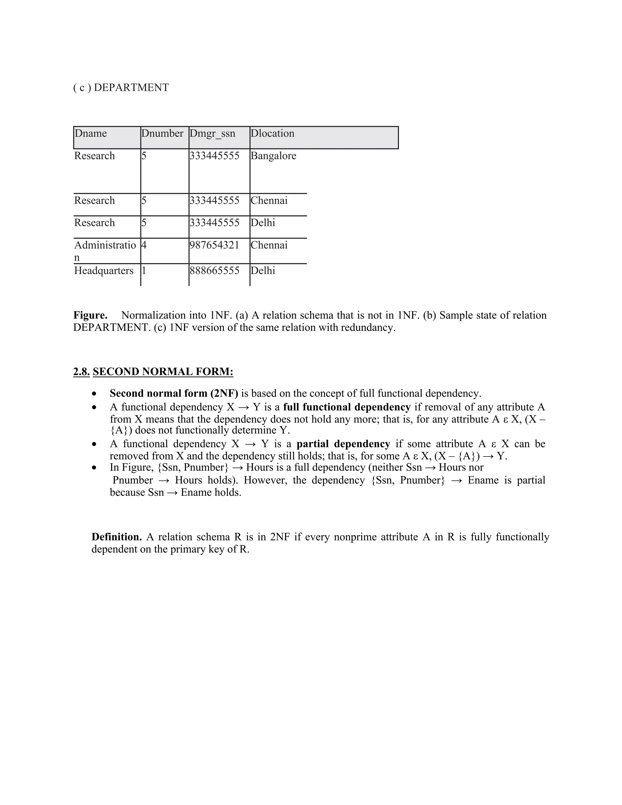
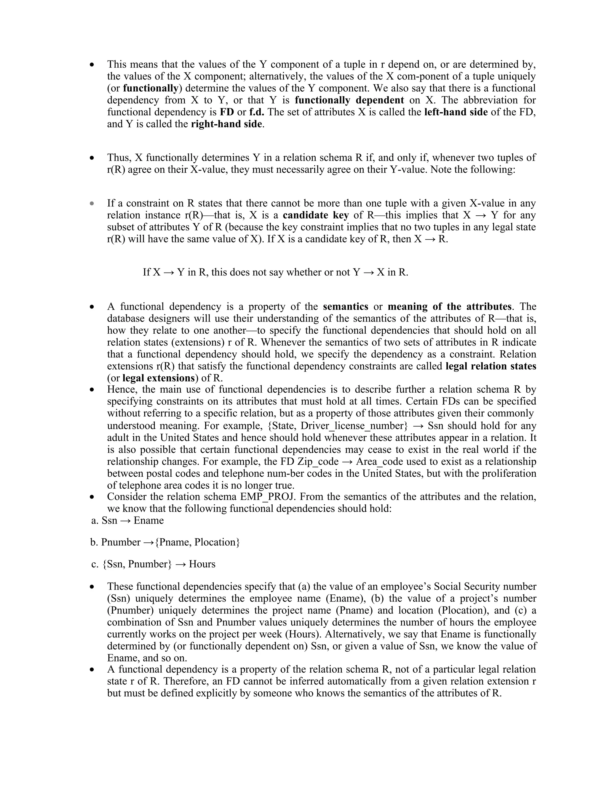
Consider the DEPARTMENT relation schema shown in Figure We assume that each
department can have a number of locations. This is not in 1NF because Dlocations is not an
atomic attribute. There are two ways we can look at the Dlocations attribute:
1) The domain of Dlocations contains atomic values, but some tuples can have a set of these values.
In this case, Dlocations is not functionally dependent on the primary key Dnumber.
2) The domain of Dlocations contains sets of values and hence is nonatomic. In this case, Dnumber
→ Dlocations because each set is considered a single member of the attribute domain.
a)
DEPARTMENT
(b)
DEPARTMENT
Dname Dnumber Dmgr_ssn Dlocations
Research 5 333445555 {Bangalore, Chennai, Delhi}
Administratio
n
4 987654321 { Chennai }
Headquarters 1 888665555 { Delhi }](https://image.slidesharecdn.com/unit2-240820061912-bfb86ab1/75/Relational-data-base-and-Er-diagema-Normalization-34-2048.jpg)