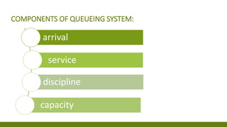
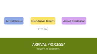
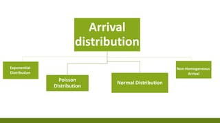
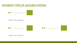
Queueing theory finallll waiting lines .pptx

MEET OUR TEAM
Presentation title 1
OLA ELNAGHY ABDELRAHMAN
METWALLY
HELMIA NOAMAN AHMED MANSOUR

MEET OUR TEAM
Presentation title 2
ABDULLAH TAREK ESLAM HAMOUDA MAZEN ELBESSA AHMED KHALED

PRESENTED TO: DR. HANAN KOUTA
QUEUEING THEORY
(WAITING LINE)

▪ Queuing theory is a branch of
applied mathematics and
operations research that focuses
on the study of waiting lines and
the underlying processes that
govern them. It provides a
systematic framework for
understanding, analyzing, and
optimizing the efficiency and
performance of systems where
customers arrive, wait in a line,
and are served by one or more
service providers.
WHAT IS QUEUEING THEORY?

capacity
COMPONENTS OF QUEUEING SYSTEM:
arrival
service
discipline

ARRIVAL PROCESS?
CONSISTS OF 3 ELEMENTS:
Arrival Rate(λ) Inter-Arrival Time(T) Arrival Distribution
(T = 1/λ)

Arrival
distribution
Poisson
Distribution
Normal Distribution
Exponential
Distribution
Non-Homogeneous
Arrival

COMMON QUEUE DISCIPLINES:
▪ First-Come-First-Served (FCFS):
▪ Priority Queuing:
-Preemptive Queues
-Non-Preemptive Queues
▪ Last-Come-First-Served (LCFS):
▪ Shortest Processing Time (SPT):
▪ Round Robin
The choice of queue
discipline can significantly
impact the system's
performance, including
waiting times and service
times.

DIFFERENT TYPES OF QUEUING SYSTEMS:
Single server, single phase
Single server, multi phase

multi server, single phase

multi server, multi phase

KENDALL NOTATION: Kendall's notation typically consists of three parts:
A represents the arrival process of
customers
A
represents the service process (e.g.,
exponential service, constant service,
etc.).
B
C represents the number of service
channels (servers) available in the
system (e.g., single-server, multi-server).
c

KENDALL NOTATION: Kendall's notation typically consists of three parts:
D describes the queue discipline
(e.g., FIFO, LIFO, priority, etc.).
D
represents the maximum system
capacity (e.g., infinite, finite, or limited
queue length).
E
G indicates whether there is a waiting
room or not (e.g., with or without a
waiting room).
G

M/M/1
M/M/c/c
M/M/∞
M/D/1
M/M/c
M/G/1
M/M/c/K

WHY?
So, WHY do we study queueing theory?
 Network Design
 Customer Service Improvement
 Computer Systems and Software Design
 Emergency Departments and health care
 Inventory Systems
 Call Centers
 Capacity Planning

CASE STUDY:
OPTIMIZING CUSTOMER SERVICE IN A RETAIL STORE USING QUEUEING
THEORY

Background:
A popular retail store with a high volume of customer foot
traffic was facing challenges in managing long queues at
the checkout counters, leading to customer dissatisfaction
and potential loss of sales. The management decided to
apply queueing theory to optimize their customer service
operations.
Objective:
The primary objective was to reduce customer waiting
times, improve overall service efficiency, and enhance
customer satisfaction without increasing operational costs.

Data Collection:
• Gathered data on customer arrival patterns throughout the day.
• Collected information on the average service time per
customer at the checkout counters.
Queueing Model
Selection:
• Selected an appropriate queueing model based on the
characteristics of the retail store's checkout system. The
Single-Server Queue model with Poisson arrival and
exponential service time distributions was deemed suitable.
Parameter
Estimation:
• Estimated parameters such as arrival rates and service
rates based on historical data.

Queueing
System
Analysis:
• Used the selected queueing model to analyze the system's
performance, including average queue length, utilization of
checkout counters, and expected waiting times.
Simulation and
Optimization:
• Employed simulation techniques to model the checkout process and
assess different scenarios.
• Explored the impact of varying the number of checkout counters and
staffing levels on customer waiting times and service efficiency.
Optimal Resource
Allocation:
• Determined the optimal number of checkout counters and staff
required to meet service level targets, balancing the cost of
additional resources against the benefits of improved customer
satisfaction.

Implementation
of Changes:
• Based on the findings from the queueing theory analysis and
simulations, the retail store management implemented changes in
the checkout process.
• Adjusted the number of open checkout counters during peak and
off-peak hours.
• Implemented a dynamic staffing model to respond to fluctuations
in customer demand.

 Reduced Waiting Times
 Improved Customer Satisfaction
 Efficient Resource Utilization
 Increased Revenue

PROBLEM (1)
A wholesale store has 2 service desks, one at each entrance of the
store. Customers arrive at each service
desk at an average of one every six minutes. The service time at
each service desk is four minutes per
customer.
a. How often is each service desk idle?
b. How many customers, on average, are waiting in line in
front of each service desk?
c. How much time does a customer spend at the service desk
(waiting plus service time)?

SOLUTION:
Data:
λ = 10 customers/hr
Service time = 4 minutes
μ = 1/service time =
(1/4)*60 = 15 customers/hr
λ /μ = 1/15 = 0.67
a. How often is each service desk idle?
A single server is idle when there are no customers
Proportion of idle time = PO
Po = 1- (λ /μ ) = 1-(0.67) = 0.33
b. How many customers, on average, are waiting in line in front
of each service desk?
Lq =
λ2
μ(μ−λ)
=
102
15(15−10)
= 1.33 𝑐𝑢𝑠𝑡𝑜𝑚𝑒𝑟𝑠
c. How much time does a customer spend at the service desk
Ws= Wq+ service time=
Wq=
𝐿𝑞
λ
=
1.33
10
= 0.133 ℎ𝑟 = 8 𝑚𝑖𝑛𝑢𝑡𝑒𝑠
Ws= 8 + 4 = 12 minutes

PROBLEM (2)
The store manager is considering consolidating the 2 service desks
into one location,
staffed by 2 clerks. The clerks will continue to work at the same
individual speed of 4
minutes per customer.
a. How many customers, on average, are waiting in line?
b. How much time does a customer spend at the service desk
c. Do you think the manager should consolidate the service
desks?

SOLUTION:
Data:
M=2
λ = 20 customers/hr
μ=15customers/hr
a. How many customers, on average, are waiting in line?
For simplicity, look in the table for the value of λ/μ that is
closest to the value we have. From the table, for λ/μ = 1.3 and
M = 2, L₁= 0.951customers
b. How much time does a customer spend at the service desk
Wq = Lq/λ = 0.954/20 = 0.0477 hr = 2.9 minutes
Ws = 2.9 + 4 = 6.9 minutes
c. Do you think the manager should consolidate the service
desks?
Yes, because the waiting time is shorter now.

PROBLEM (3)
A clinic has two general practitioners who see patients daily. An
average of 6 patients arrives at the clinic every hour (Poisson
distributed). Each doctor spends an average of 15 minutes
(exponentially distributed) with a patient. The patient wait in a
waiting
area until one of the doctors is able to see him. However, since
patients typically do not feel well when they come to the clinic, the
doctors do not believe it is good practice to have a patient wait
longer than an average of 15 minutes.
Should this clinic add a third doctor? How would this alleviate the waiting problem?

SOLUTION:
DATA:
M=2
X = 6 patients/hr
Service time = 15
minutes
μ = 1/service time = (1/15)*60 = 4 patients/hr
λ/μ = 6/4 =1.5
The clinic has a policy that patients should not wait more than
15 minutes before seeing a doctor To answer the question, we
need to know the current waiting time and compare it to the
threshold.
From the table, for λ/μ= 1.5 and M = 2,
Lq = 1.929 patients
Wq = Lq/λ = 1.929/6 = 0.3215 hr = 19.3 minutes > 15 minutes
So, add a doctor.
M now is 3
From the table, for λ/μ = 1.5 and M = 3,
Lq = 0.237 patients
Wq = Lq/λ = 0.237/6 = 0.0395 hr = 2.4 minutes < 15 minutesBy
adding one doctor, we reduce the waiting time by (19.3-2.4) =
16.9 minutes

PROBLEM (3)
A service counter employs two servers. On average a server requires
8 minutes to
process a customer and service times follow an exponential
distribution. Customers
arrive at the counter at the rate of 12 per hour according to a Poisson
distribution.
Determine the following.
a. On average, the total number of customers in the system
b. The average number of customers waiting to be served
c. The average amount of time, in minutes, spent in the system
d. The probability that an arriving customer must wait for
service
e. The probability that two customers are waiting in line

SOLUTION:
Data:
M = 2λ = 12 customers/hr
(1/8)*60 = 7.5
customers/hr
λ/μ = 12/7.5 = 1.6
a. On average, the total number of customers in the system
Lq = 2.844 customers
Ls = Lq + λ/μ= 2.84 + 1.6 = 4.44 customers
b. The average number of customers waiting to be served
This is Lq which is 2.84 customers
c. The average amount of time, in minutes, spent in the system
Ws = Wq + service time
Wq = Lq/λ = 2.84/12 = 0.237 hr = 14.2 minutes
Ws = 14.2 + 8 = 22.2 minutes

SOLUTION:
Data:
M = 2λ = 12 customers/hr
(1/8)*60 = 7.5
customers/hrλ/μ = 12/7.5
= 1.6
d. The probability that an arriving customer must wait for
service
Pw = P₂ + P3 + ... = 1 - (Po+P₁)
Po= 0.111(/μ)"For n ≤ M, Pn = (λ/μ)*n/n! X Po
P₁ =(1.6)*1/1! X 0.111 = 0.1776
Pw=1- (0.111 + 0.1776) = 1- 0.2886 = 0.7114
e. The probability that two customers are waiting in line
P(n = 2 in line) = P(n = 4 in system) = P4
For n > M, Pn = (λ/μ)*n / M! M*n-M X PO
P4= (1.6)*4 / 2! 2*4-2 X 0.111= 0.0909

• The costs of waiting in line:
1-paying idle employees while they are in line waiting for
something they need. (waiting for parts, supplies, deliveries,
etc.)
2-Unusable (unproductive) equipment awaiting repairs
EG: Broken assembly line machinery.
3-Losing customers because of long lines
-Reneging: Customers get tired of waiting and leave
-Balking: Customers see a long line and don't get in line.

• The cost of providing service to the line
● Paying people to service the customers in line
● Customers can be people, machines, or other objects
needing service.
● Paying repairmen to fix broken machines
Paying dock workers to load and unload trucks
● Paying customer-service people
● Using more production people to speed up the line
• Leasing of service equipment and facilities
Paying checkout cashiers

PROBLEM
In the Burger Dome restaurant problem, the waiting cost would be the cost per minute
for a customer waiting for service. This cost is not a direct cost to Burger Dome.
However, if Burger Dome ignores this cost and allows long waiting lines, customers
ultimately will take their business elsewhere. Thus, Burger Dome will experience lost sales and, in
effect, incur a cost.
In the Burger Dome problem, The service cost would include the server's wages,
benefits, and any other direct costs associated with establishing a server. At Burger
Dome, this cost is estimated to be $10 per hour.
Assume that Burger Dome is willing to assign a cost of $15 per hour for customer
waiting time.
Assume in Single-server system (L = 3 customers)
Two-server system (L = 0.8727 customer)

PROBLEM
Single-server system (L = 3 customers): TC = CwL+ Cşk
= 15(3) + 10(1) = $55.00 per hour
Solution
Two-server system (L = 0.8727 customer):
TC=CwL+ Cşk
= 15(0.8727) + 10(2) = $33.09 per hour

Queueing theory finallll waiting lines .pptx

More Related Content

Similar to Queueing theory finallll waiting lines .pptx

Recently uploaded

Queueing theory finallll waiting lines .pptx