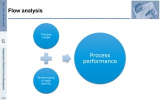
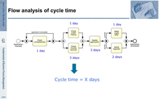
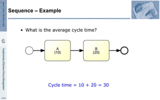
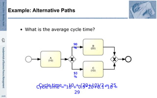
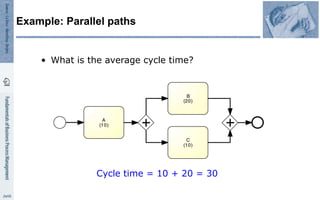
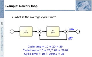
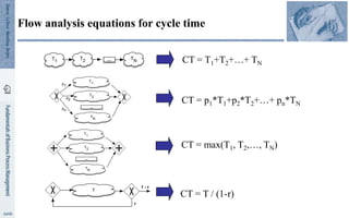
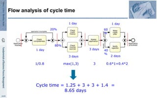
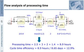
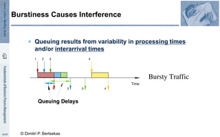
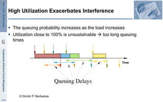
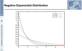
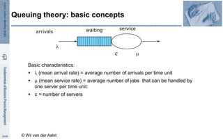
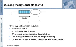
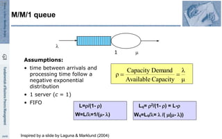
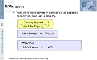
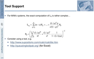
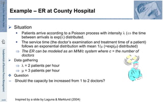
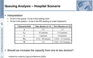
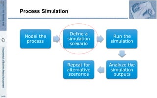
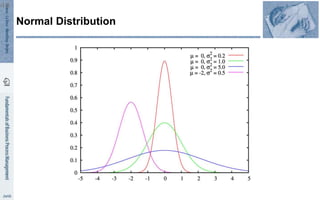
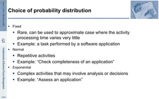
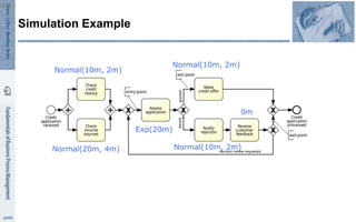
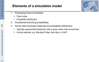
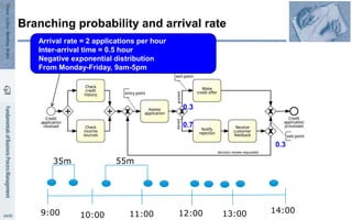
SlideShare a Scribd company logo
1 of 66
Contents
1. Flow Analysis
2. Queuing Analysis
3. Simulation
4. Recap
SEITE 1
Chapter 7: Quantitative Process Analysis
Process
discovery
Process
identification
Process
analysis
Process
implementation
Process
monitoring
Process
redesign
Process architecture
As-is process
model
Insights on
weaknesses and
their impact
To-be process
model
Executable
process
model
Conformance and
performance
insights
Process Analysis in the BPM Lifecycle
Define Vision Develop Strategy Implement
Strategy
Manage Personnel Manage Assets
Management Processes
Core Processes
Support Processes
Manage Risk
Manage
Information
Procure
Materials
Procure
Products
Market
Products
Deliver
Products
Manage
Customer
Service
les for BPM lifecycle and process mining
C
1.5h
B
15h
D
E
2h
C D
A B E
A
3m
35h 30h
15m
10m
10min
5m
5m 10m
30m
Contents
1. Flow Analysis
2. Queuing Analysis
3. Simulation
4. Recap
SEITE 3
Chapter 7: Quantitative Process Analysis
Process
model
Performance
of each
activity
Process
performance
Flow analysis
4
Refresher: Process performance measures
Process
perform
ance
Time
Cost
Quality
Processing
time
Waiting
time
Cycle
time
Common time-related measures
6
Time taken by
value-adding
activities
Time between start
and completion of a
process instance
Time taken by
non-value-adding
activities
Processi
ng Time
Cycle
Time
Cycle
Time
Efficienc
y
Cycle time efficiency
7
Flow analysis of cycle time
8
1 day
1 day
3 days
3 days
1 day
2 days
Cycle time = X days
Sequence – Example
9
• What is the average cycle time?
Cycle time = 10 + 20 = 30
50
%
50
%
90
%
10
%
Cycle time = 10 + (20+10)/2 = 25
Cycle time = 10 + 0.9*20+0.1*10 =
29
Example: Alternative Paths
• What is the average cycle time?
Cycle time = 10 + 20 = 30
Example: Parallel paths
• What is the average cycle time?
Example: Rework loop
100%
0%
Cycle time = 10 + 20 = 30
1%
99%
Cycle time = 10 + 20/0.01 = 2010
80%
20%
Cycle time = 10 + 20/0.8 = 35
Flow analysis equations for cycle time
CT = max(T1, T2,…, TN)
CT = p1*T1+p2*T2+…+ pn*TN
CT = T / (1-r)
CT = T1+T2+…+ TN
T
r
1 - r
T1
...
T2
TN
T1
...
T2
TN
p2
pn
p1
T1 ...
T2 TN
Flow analysis of cycle time
14
1 day
1 day
3 days
3 days
1 day
2 days
Cycle time = 1.25 + 3 + 3 + 1.4 =
8.65 days
20% 60
%
1/0.8 max(1,3) 3 0.6*1+0.4*2
80%
40
%
Flow analysis of processing time
15
2 hours
0.5 hour
2 hours
2
hours
0.5 mins.
Processing time = 2.5 + 3 + 2 + 1.4 = 8.9 hours
20% 60
%
2/0.8 max(0.5,3) 2 0.6*2+0.4*0.5
80%
40
%
3 hours
Cycle time efficiency = 8.9 hours / 8.65 days = 12.9%
Flow analysis: scope and limitations
 We have seen how to use flow analysis for processing & cycle time calculation
 Flow analysis can also be applied to calculate:
 The average cost of process instances (assuming we know the cost of each activity)
 Cf. Section 7.1.6
 The number of times on average each activity is executed
 Can be used to calculate the “unit load” of each task, the resource utilization of each
resource pool, and the theoretical capacity of an “as is” process
 Cf. Section 7.1.5
 But flow analysis has some fundamental limitations…
Limitation 1: Not all Models are Structured
 Cycle time analysis does not consider:
 The rate at which new process instances are created (arrival rate)
 The number of available resources
 Higher arrival rate at fixed resource capacity
 high resource contention
 higher activity waiting times (longer queues)
 higher activity cycle time
 higher overall cycle time
 The slower you are, the more people have to queue up…
 and vice-versa
Limitation 2: Fixed arrival rate capacity
Time spent
per
resource on
process
work
Time
available
per
resource for
process
work
Resource
utilization
Resource utilization
19
Resource utilization = 60%
 on average resources are idle 40% of
their allocated time
Resource
utilization Waiting
time
Resource utilization vs. waiting time
20
Typically, when resource utilization > 90%
 Waiting time increases steeply
 WIP = (average) Work-In-Process
 Number of cases that are running (started but not yet completed)
 E.g. # of active and unfilled orders in an order-to-cash process
 WIP is a form of waste (cf. 7+1 sources of waste)
 Little’s Formula: WIP = ·CT
  = arrival rate (number of new cases per time unit)
 CT = cycle time
Interlude:
Cycle Time & Work-In-Progress
Exercise
A fast-food restaurant receives on average 1200
customers per day (between 10:00 and 22:00). During
peak times (12:00-15:00 and 18:00-21:00), the restaurant
receives around 900 customers in total, and 90 customers
can be found in the restaurant (on average) at a given
point in time. At non-peak times, the restaurant receives
300 customers in total, and 30 customers can be found in
the restaurant (on average) at a given point in time.
1. What is the average time that a customer spends in the
restaurant during peak times?
2. What is the average time that a customer spends in the
restaurant during non-peak times?
Exercise (cont.)
3. The restaurant plans to launch a marketing campaign to attract more customers.
However, the restaurant’s capacity is limited and becomes too full during peak
times. What can the restaurant do to address this issue without investing in
extending its building?
Contents
1. Flow Analysis
2. Queuing Analysis
3. Simulation
4. Recap
SEITE 24
Chapter 7: Quantitative Process Analysis
 Capacity problems are common and a key driver of process
redesign
 Need to balance the cost of increased capacity against the gains of
increased productivity and service
 Queuing and waiting time analysis is particularly important in
service systems
 Large costs of waiting and/or lost sales due to waiting
 Example – Emergency Room (ER) at a Hospital
 Patients arrive by ambulance or by their own accord
 One doctor is always on duty
 More patients seeks help  longer waiting times
 Should we increase the capacity from one to two doctors?
Queuing Analysis
Inspired by an example by Laguna & Marklund (2004)
25
If arrivals are regular or sufficiently spaced apart, no queuing delay
occurs
Delay is Caused by Job Interference
Deterministic traffic
Variable but
spaced apart
traffic
© Dimitri P. Bertsekas
26
Burstiness Causes Interference
 Queuing results from variability in processing times
and/or interarrival times
© Dimitri P. Bertsekas
27
 The queuing probability increases as the load increases
 Utilization close to 100% is unsustainable  too long queuing
times
High Utilization Exacerbates Interference
© Dimitri P. Bertsekas
28
 Common arrival assumption in many queuing and simulation
models
 The times between arrivals are independent, identically
distributed and exponential
 P (arrival < t) = 1 – e-λt
 This distribution is applicable when the next arrival (i.e. the
next creation of a case) does not depend on how long ago
the previous arrival occurred
 In other words, the creation of a case is independent of the creation of
other cases.
The Poisson Process
Inspired by slide by Laguna & Marklund (2004)
29
Negative Exponential Distribution
30
Basic characteristics:
  (mean arrival rate) = average number of arrivals per time unit
 m (mean service rate) = average number of jobs that can be handled by
one server per time unit:
 c = number of servers
Queuing theory: basic concepts
arrivals waiting service

m
c
© Wil van der Aalst
31
Given  , m and c, we can calculate :
 occupation rate: r
 Wq = average time in queue
 W = average system in system (i.e. cycle time)
 Lq = average number in queue (i.e. length of queue)
 L = average number in system average (i.e. Work-in-Progress)
Queuing theory concepts (cont.)

m
c
Wq,Lq
W,L
© Wil van der Aalst
32
M/M/1 queue

m
1
Assumptions:
• time between arrivals and
processing time follow a
negative exponential
distribution
• 1 server (c = 1)
• FIFO
L=r/(1- r) Lq= r2/(1- r) = L-r
W=L/=1/(m- ) Wq=Lq/=  /( m(m- ))
μ
λ
Capacity
Available
Demand
Capacity
ρ 

33
Inspired by a slide by Laguna & Marklund (2004)
m



r
*
c
Capacity
Available
Demand
Capacity
• Now there are c servers in parallel, so the expected
capacity per time unit is then c*m
W=Wq+(1/m)
Little’s Formula  Wq=Lq/
Little’s Formula  L=W
Inspired by a slide by Laguna & Marklund (2004)
M/M/c queue
34
 For M/M/c systems, the exact computation of Lq is rather complex…
 Consider using a tool, e.g.
 http://www.supositorio.com/rcalc/rcalclite.htm
 http://queueingtoolpak.org/ (for Excel)
Tool Support
0
2
c
c
n
n
q P
)
1
(
!
c
)
/
(
...
P
)
c
n
(
L
r

r
m




 


1
c
1
c
0
n
n
0
)
c
/(
(
1
1
!
c
)
/
(
!
n
)
/
(
P











m



m


m

 
35
 Situation
 Patients arrive according to a Poisson process with intensity  ( the time
between arrivals is exp() distributed.
 The service time (the doctor’s examination and treatment time of a patient)
follows an exponential distribution with mean 1/m (=exp(m) distributed)
 The ER can be modeled as an M/M/c system where c = the number of
doctors
 Data gathering
  = 2 patients per hour
 m = 3 patients per hour
 Question
– Should the capacity be increased from 1 to 2 doctors?
Example – ER at County Hospital
36
Inspired by a slide by Laguna & Marklund (2004)
 Interpretation
 To be in the queue = to be in the waiting room
 To be in the system = to be in the ER (waiting or under treatment)
 Should we increase the capacity from one to two doctors?
Queuing Analysis – Hospital Scenario
Characteristic One doctor (c=1) Two Doctors (c=2)
r 2/3 1/3
Lq 4/3 patients 1/12 patients
L 2 patients 3/4 patients
Wq 2/3 h = 40 minutes 1/24 h = 2.5 minutes
W 1 h 3/8 h = 22.5 minutes
37
Inspired by a slide by Laguna & Marklund (2004)
 Can be used to analyze waiting times (and hence cycle times), but not cost or
quality measures
 Suitable for analyzing one single activity at a time, performed by one single
resource pool. Not suitable for analyzing end-to-end processes consisting of
multiple activities performed by multiple resource pools.
 These limitations are addressed by process simulation
Limitations of basic queuing models
38
Contents
1. Value-Added Analysis
2. Queuing analysis
3. Simulation
4. Recap
SEITE 39
Chapter 7: Quantitative Process Analysis
 Versatile quantitative analysis method for
 As-is analysis
 What-if analysis
 In a nutshell:
 Run a large number of process instances
 Gather performance data (cost, time, resource usage)
 Calculate statistics from the collected data
Process Simulation
40
Process Simulation
Model the
process
Define a
simulation
scenario
Run the
simulation
Analyze the
simulation
outputs
Repeat for
alternative
scenarios
41
Example
42
Example
43
Elements of a simulation scenario
1. Processing times of activities
 Fixed value
 Probability distribution
44
Exponential Distribution
45
Normal Distribution
46
 Fixed
 Rare, can be used to approximate case where the activity
processing time varies very little
 Example: a task performed by a software application
 Normal
 Repetitive activities
 Example: “Check completeness of an application”
 Exponential
 Complex activities that may involve analysis or decisions
 Example: “Assess an application”
Choice of probability distribution
47
Simulation Example
Exp(20m)
Normal(20m, 4m)
Normal(10m, 2m)
Normal(10m, 2m)
Normal(10m, 2m)
0m
48
Elements of a simulation model
1. Processing times of activities
 Fixed value
 Probability distribution
2. Conditional branching probabilities
3. Arrival rate of process instances and probability distribution
 Typically exponential distribution with a given mean inter-arrival time
 Arrival calendar, e.g. Monday-Friday, 9am-5pm, or 24/7
49
Branching probability and arrival rate
Arrival rate = 2 applications per hour
Inter-arrival time = 0.5 hour
Negative exponential distribution
From Monday-Friday, 9am-5pm
0.3
0.7
0.3
9:00 10:00 11:00 12:00 13:00 14:00
35m 55m
50
Elements of a simulation model
1. Processing times of activities
 Fixed value
 Probability distribution
2. Conditional branching probabilities
3. Arrival rate of process instances
 Typically exponential distribution with a given mean inter-arrival time
 Arrival calendar, e.g. Monday-Friday, 9am-5pm, or 24/7
4. Resource pools
51
Resource pools
 Name
 Size of the resource pool
 Cost per time unit of a resource in the pool
 Availability of the pool (working calendar)
 Examples
 Clerk Credit Officer
 € 25 per hour € 25 per hour
 Monday-Friday, 9am-5pm Monday-Friday, 9am-5pm
 In some tools, it is possible to define cost and calendar per resource,
rather than for entire resource pool
52
Elements of a simulation model
1. Processing times of activities
 Fixed value
 Probability distribution
2. Conditional branching probabilities
3. Arrival rate of process instances and probability distribution
 Typically exponential distribution with a given mean inter-arrival time
 Arrival calendar, e.g. Monday-Friday, 9am-5pm, or 24/7
4. Resource pools
5. Assignment of tasks to resource pools
53
Resource pool assignment
Officer
Clerk
Clerk Officer
Officer
Syste
m
54
Process Simulation
Model the
process
Define a
simulation
scenario
Run the
simulation
Analyze the
simulation
outputs
Repeat for
alternative
scenarios
✔ ✔ ✔
55
Output: Performance measures & histograms
56
Process Simulation
Model the
process
Define a
simulation
scenario
Run the
simulation
Analyze the
simulation
outputs
Repeat for
alternative
scenarios
✔ ✔ ✔
✔
57
Tools for Process Simulation
 ARIS
 Bizagi Process Modeler
 ITP Commerce Process Modeler for Visio
 Logizian
 Oracle BPA
 Progress Savvion Process Modeler
 ProSim
 Signavio + BIMP
58
BIMP – bimp.cs.ut.ee
 Accepts standard BPMN 2.0 as input
 Simple form-based interface to enter simulation scenario
 Produces KPIs + simulation logs in MXML format
 Simulation logs can be imported to the ProM process mining tool
59
BIMP Demo
60
https://www.youtube.com/watch?v=TjXl6yASCSc
 Stochasticity
 Data quality pitfalls
 Simplifying assumptions
Pitfalls of simulation
61
 Simulation results may differ from one run to another
 Make the simulation tiemframe long enough to cover weekly and seasonal
variability, where applicable
 Use multiple simulation runs
 Average results of multiple runs, compute confidence intervals
Stochasticity
62
 Simulation results are only as trustworthy as the input data
 Rely as little as possible on “guesstimates”
 Use input analysis
 Deriver simulation scenario parameters from numbers in the scenario
 Use statistical tools to check fit the probability distributions
 Simulate the “as is” scenario and cross-check results against actual observations
Data quality pitfalls
63
 That the process model is always followed to the letter
 No deviations
 No workarounds
 That there is no multi-tasking (the same resource performs multiple tasks
concurrently) nor batching (tasks being accumulated and performed in a single go)
 That resources work constantly and non-stop
 Every day is the same!
 No tiredness effects
 No distractions beyond “stochastic” ones
Simulation assumptions
64
Contents
1. Value-Added Analysis
2. Queuing analysis
3. Simulation
4. Recap
SEITE 65
Chapter 7: Quantitative Process Analysis
 Assuming we have performance measures for each activity in a process, flow
analysis allows us to calculate the following performance measures for an “as is”
process:
 Cycle time, processing times, cycle time efficiency of a process
 Average cost per process instance
 It can also be used to calculate the theoretical capacity of an “as is” process and
the resource utilization of resource pools
 But it is not suitable for “what if” analysis
 Queing analysis is a suitable technique for “what if” analysis of waiting times and
cycle times, suitable for analyzing individual activities performed by one resource
pool
 Simulation is a versatile technique for “what if” analysis of entire processes,
covering waiting times, cycle times, and costs.
 Particularly useful for identifying bottlenecks
SLIDE 66
Recap

More Related Content

Similar to Flow queue analysis co4.pptx business process management

Queuing theory and its applications
Queuing theory and its applicationsQueuing theory and its applications
Queuing theory and its applicationsDebasisMohanty37
 
Waiting Line Management
Waiting Line Management Waiting Line Management
Waiting Line Management Joshua Miranda
 
Comparision of different Round Robin Scheduling Algorithm using Dynamic Time ...
Comparision of different Round Robin Scheduling Algorithm using Dynamic Time ...Comparision of different Round Robin Scheduling Algorithm using Dynamic Time ...
Comparision of different Round Robin Scheduling Algorithm using Dynamic Time ...Editor IJMTER
 
In designing a lean production facility layout
In designing a lean production facility layoutIn designing a lean production facility layout
In designing a lean production facility layoutjohann11371
 
Which of the following basic types of production layout
Which of the following basic types of production layoutWhich of the following basic types of production layout
Which of the following basic types of production layoutjohann11372
 
An Introduction to Operations Management
An Introduction to Operations ManagementAn Introduction to Operations Management
An Introduction to Operations ManagementChristian Reinboth
 
Which of the following is not a problem definition tool
Which of the following is not a problem definition toolWhich of the following is not a problem definition tool
Which of the following is not a problem definition tooljohann11374
 
Simulation and modeling
Simulation and modelingSimulation and modeling
Simulation and modelingHabibur Rahman
 
From an operational perspective, yield management is most effective under whi...
From an operational perspective, yield management is most effective under whi...From an operational perspective, yield management is most effective under whi...
From an operational perspective, yield management is most effective under whi...johann11371
 
Cost minimization model
Cost minimization modelCost minimization model
Cost minimization modelrowell balala
 
A company must perform a maintenance project consisting
A company must perform a maintenance project consistingA company must perform a maintenance project consisting
A company must perform a maintenance project consistingjohann11369
 
Queing theory and delay analysis
Queing theory and delay analysisQueing theory and delay analysis
Queing theory and delay analysisPriyanka Negi
 
Which of the following is an input to the master production schedule (mps)
Which of the following is an input to the master production schedule (mps)Which of the following is an input to the master production schedule (mps)
Which of the following is an input to the master production schedule (mps)johann11374
 
Which of the following approaches to service design
Which of the following approaches to service designWhich of the following approaches to service design
Which of the following approaches to service designjohann11372
 
Supporting Facility and Process Flows Chapter 7McG.docx
Supporting Facility and Process Flows Chapter 7McG.docxSupporting Facility and Process Flows Chapter 7McG.docx
Supporting Facility and Process Flows Chapter 7McG.docxmattinsonjanel
 
An advantage of a make to-stock process is which of the following
An advantage of a make to-stock process is which of the followingAn advantage of a make to-stock process is which of the following
An advantage of a make to-stock process is which of the followingjohann11370
 
Which of the following is a focusing step
Which of the following is a focusing stepWhich of the following is a focusing step
Which of the following is a focusing stepjohann11373
 

Similar to Flow queue analysis co4.pptx business process management (20)

Intro DES-Capacity
Intro DES-CapacityIntro DES-Capacity
Intro DES-Capacity
 
Queuing theory and its applications
Queuing theory and its applicationsQueuing theory and its applications
Queuing theory and its applications
 
Waiting Line Management
Waiting Line Management Waiting Line Management
Waiting Line Management
 
QUEUEING THEORY
QUEUEING THEORYQUEUEING THEORY
QUEUEING THEORY
 
Comparision of different Round Robin Scheduling Algorithm using Dynamic Time ...
Comparision of different Round Robin Scheduling Algorithm using Dynamic Time ...Comparision of different Round Robin Scheduling Algorithm using Dynamic Time ...
Comparision of different Round Robin Scheduling Algorithm using Dynamic Time ...
 
In designing a lean production facility layout
In designing a lean production facility layoutIn designing a lean production facility layout
In designing a lean production facility layout
 
Which of the following basic types of production layout
Which of the following basic types of production layoutWhich of the following basic types of production layout
Which of the following basic types of production layout
 
An Introduction to Operations Management
An Introduction to Operations ManagementAn Introduction to Operations Management
An Introduction to Operations Management
 
Which of the following is not a problem definition tool
Which of the following is not a problem definition toolWhich of the following is not a problem definition tool
Which of the following is not a problem definition tool
 
Applying Lean in Pathology
Applying Lean in PathologyApplying Lean in Pathology
Applying Lean in Pathology
 
Simulation and modeling
Simulation and modelingSimulation and modeling
Simulation and modeling
 
From an operational perspective, yield management is most effective under whi...
From an operational perspective, yield management is most effective under whi...From an operational perspective, yield management is most effective under whi...
From an operational perspective, yield management is most effective under whi...
 
Cost minimization model
Cost minimization modelCost minimization model
Cost minimization model
 
A company must perform a maintenance project consisting
A company must perform a maintenance project consistingA company must perform a maintenance project consisting
A company must perform a maintenance project consisting
 
Queing theory and delay analysis
Queing theory and delay analysisQueing theory and delay analysis
Queing theory and delay analysis
 
Which of the following is an input to the master production schedule (mps)
Which of the following is an input to the master production schedule (mps)Which of the following is an input to the master production schedule (mps)
Which of the following is an input to the master production schedule (mps)
 
Which of the following approaches to service design
Which of the following approaches to service designWhich of the following approaches to service design
Which of the following approaches to service design
 
Supporting Facility and Process Flows Chapter 7McG.docx
Supporting Facility and Process Flows Chapter 7McG.docxSupporting Facility and Process Flows Chapter 7McG.docx
Supporting Facility and Process Flows Chapter 7McG.docx
 
An advantage of a make to-stock process is which of the following
An advantage of a make to-stock process is which of the followingAn advantage of a make to-stock process is which of the following
An advantage of a make to-stock process is which of the following
 
Which of the following is a focusing step
Which of the following is a focusing stepWhich of the following is a focusing step
Which of the following is a focusing step
 

Recently uploaded

HARMONY IN THE HUMAN BEING - Unit-II UHV-2
HARMONY IN THE HUMAN BEING - Unit-II UHV-2HARMONY IN THE HUMAN BEING - Unit-II UHV-2
HARMONY IN THE HUMAN BEING - Unit-II UHV-2RajaP95
 
Microscopic Analysis of Ceramic Materials.pptx
Microscopic Analysis of Ceramic Materials.pptxMicroscopic Analysis of Ceramic Materials.pptx
Microscopic Analysis of Ceramic Materials.pptxpurnimasatapathy1234
 
VIP Call Girls Service Kondapur Hyderabad Call +91-8250192130
VIP Call Girls Service Kondapur Hyderabad Call +91-8250192130VIP Call Girls Service Kondapur Hyderabad Call +91-8250192130
VIP Call Girls Service Kondapur Hyderabad Call +91-8250192130Suhani Kapoor
 
Call Girls Delhi {Jodhpur} 9711199012 high profile service
Call Girls Delhi {Jodhpur} 9711199012 high profile serviceCall Girls Delhi {Jodhpur} 9711199012 high profile service
Call Girls Delhi {Jodhpur} 9711199012 high profile servicerehmti665
 
Study on Air-Water & Water-Water Heat Exchange in a Finned Tube Exchanger
Study on Air-Water & Water-Water Heat Exchange in a Finned Tube ExchangerStudy on Air-Water & Water-Water Heat Exchange in a Finned Tube Exchanger
Study on Air-Water & Water-Water Heat Exchange in a Finned Tube ExchangerAnamika Sarkar
 
main PPT.pptx of girls hostel security using rfid
main PPT.pptx of girls hostel security using rfidmain PPT.pptx of girls hostel security using rfid
main PPT.pptx of girls hostel security using rfidNikhilNagaraju
 
SPICE PARK APR2024 ( 6,793 SPICE Models )
SPICE PARK APR2024 ( 6,793 SPICE Models )SPICE PARK APR2024 ( 6,793 SPICE Models )
SPICE PARK APR2024 ( 6,793 SPICE Models )Tsuyoshi Horigome
 
Call Girls Narol 7397865700 Independent Call Girls
Call Girls Narol 7397865700 Independent Call GirlsCall Girls Narol 7397865700 Independent Call Girls
Call Girls Narol 7397865700 Independent Call Girlsssuser7cb4ff
 
Heart Disease Prediction using machine learning.pptx
Heart Disease Prediction using machine learning.pptxHeart Disease Prediction using machine learning.pptx
Heart Disease Prediction using machine learning.pptxPoojaBan
 
VICTOR MAESTRE RAMIREZ - Planetary Defender on NASA's Double Asteroid Redirec...
VICTOR MAESTRE RAMIREZ - Planetary Defender on NASA's Double Asteroid Redirec...VICTOR MAESTRE RAMIREZ - Planetary Defender on NASA's Double Asteroid Redirec...
VICTOR MAESTRE RAMIREZ - Planetary Defender on NASA's Double Asteroid Redirec...VICTOR MAESTRE RAMIREZ
 
(ANVI) Koregaon Park Call Girls Just Call 7001035870 [ Cash on Delivery ] Pun...
(ANVI) Koregaon Park Call Girls Just Call 7001035870 [ Cash on Delivery ] Pun...(ANVI) Koregaon Park Call Girls Just Call 7001035870 [ Cash on Delivery ] Pun...
(ANVI) Koregaon Park Call Girls Just Call 7001035870 [ Cash on Delivery ] Pun...ranjana rawat
 
Current Transformer Drawing and GTP for MSETCL
Current Transformer Drawing and GTP for MSETCLCurrent Transformer Drawing and GTP for MSETCL
Current Transformer Drawing and GTP for MSETCLDeelipZope
 
Biology for Computer Engineers Course Handout.pptx
Biology for Computer Engineers Course Handout.pptxBiology for Computer Engineers Course Handout.pptx
Biology for Computer Engineers Course Handout.pptxDeepakSakkari2
 
Software and Systems Engineering Standards: Verification and Validation of Sy...
Software and Systems Engineering Standards: Verification and Validation of Sy...Software and Systems Engineering Standards: Verification and Validation of Sy...
Software and Systems Engineering Standards: Verification and Validation of Sy...VICTOR MAESTRE RAMIREZ
 
(MEERA) Dapodi Call Girls Just Call 7001035870 [ Cash on Delivery ] Pune Escorts
(MEERA) Dapodi Call Girls Just Call 7001035870 [ Cash on Delivery ] Pune Escorts(MEERA) Dapodi Call Girls Just Call 7001035870 [ Cash on Delivery ] Pune Escorts
(MEERA) Dapodi Call Girls Just Call 7001035870 [ Cash on Delivery ] Pune Escortsranjana rawat
 
Application of Residue Theorem to evaluate real integrations.pptx
Application of Residue Theorem to evaluate real integrations.pptxApplication of Residue Theorem to evaluate real integrations.pptx
Application of Residue Theorem to evaluate real integrations.pptx959SahilShah
 
Artificial-Intelligence-in-Electronics (K).pptx
Artificial-Intelligence-in-Electronics (K).pptxArtificial-Intelligence-in-Electronics (K).pptx
Artificial-Intelligence-in-Electronics (K).pptxbritheesh05
 

Recently uploaded (20)

HARMONY IN THE HUMAN BEING - Unit-II UHV-2
HARMONY IN THE HUMAN BEING - Unit-II UHV-2HARMONY IN THE HUMAN BEING - Unit-II UHV-2
HARMONY IN THE HUMAN BEING - Unit-II UHV-2
 
★ CALL US 9953330565 ( HOT Young Call Girls In Badarpur delhi NCR
★ CALL US 9953330565 ( HOT Young Call Girls In Badarpur delhi NCR★ CALL US 9953330565 ( HOT Young Call Girls In Badarpur delhi NCR
★ CALL US 9953330565 ( HOT Young Call Girls In Badarpur delhi NCR
 
Microscopic Analysis of Ceramic Materials.pptx
Microscopic Analysis of Ceramic Materials.pptxMicroscopic Analysis of Ceramic Materials.pptx
Microscopic Analysis of Ceramic Materials.pptx
 
VIP Call Girls Service Kondapur Hyderabad Call +91-8250192130
VIP Call Girls Service Kondapur Hyderabad Call +91-8250192130VIP Call Girls Service Kondapur Hyderabad Call +91-8250192130
VIP Call Girls Service Kondapur Hyderabad Call +91-8250192130
 
young call girls in Rajiv Chowk🔝 9953056974 🔝 Delhi escort Service
young call girls in Rajiv Chowk🔝 9953056974 🔝 Delhi escort Serviceyoung call girls in Rajiv Chowk🔝 9953056974 🔝 Delhi escort Service
young call girls in Rajiv Chowk🔝 9953056974 🔝 Delhi escort Service
 
Call Girls Delhi {Jodhpur} 9711199012 high profile service
Call Girls Delhi {Jodhpur} 9711199012 high profile serviceCall Girls Delhi {Jodhpur} 9711199012 high profile service
Call Girls Delhi {Jodhpur} 9711199012 high profile service
 
Study on Air-Water & Water-Water Heat Exchange in a Finned Tube Exchanger
Study on Air-Water & Water-Water Heat Exchange in a Finned Tube ExchangerStudy on Air-Water & Water-Water Heat Exchange in a Finned Tube Exchanger
Study on Air-Water & Water-Water Heat Exchange in a Finned Tube Exchanger
 
main PPT.pptx of girls hostel security using rfid
main PPT.pptx of girls hostel security using rfidmain PPT.pptx of girls hostel security using rfid
main PPT.pptx of girls hostel security using rfid
 
SPICE PARK APR2024 ( 6,793 SPICE Models )
SPICE PARK APR2024 ( 6,793 SPICE Models )SPICE PARK APR2024 ( 6,793 SPICE Models )
SPICE PARK APR2024 ( 6,793 SPICE Models )
 
Call Girls Narol 7397865700 Independent Call Girls
Call Girls Narol 7397865700 Independent Call GirlsCall Girls Narol 7397865700 Independent Call Girls
Call Girls Narol 7397865700 Independent Call Girls
 
Heart Disease Prediction using machine learning.pptx
Heart Disease Prediction using machine learning.pptxHeart Disease Prediction using machine learning.pptx
Heart Disease Prediction using machine learning.pptx
 
VICTOR MAESTRE RAMIREZ - Planetary Defender on NASA's Double Asteroid Redirec...
VICTOR MAESTRE RAMIREZ - Planetary Defender on NASA's Double Asteroid Redirec...VICTOR MAESTRE RAMIREZ - Planetary Defender on NASA's Double Asteroid Redirec...
VICTOR MAESTRE RAMIREZ - Planetary Defender on NASA's Double Asteroid Redirec...
 
(ANVI) Koregaon Park Call Girls Just Call 7001035870 [ Cash on Delivery ] Pun...
(ANVI) Koregaon Park Call Girls Just Call 7001035870 [ Cash on Delivery ] Pun...(ANVI) Koregaon Park Call Girls Just Call 7001035870 [ Cash on Delivery ] Pun...
(ANVI) Koregaon Park Call Girls Just Call 7001035870 [ Cash on Delivery ] Pun...
 
Current Transformer Drawing and GTP for MSETCL
Current Transformer Drawing and GTP for MSETCLCurrent Transformer Drawing and GTP for MSETCL
Current Transformer Drawing and GTP for MSETCL
 
Call Us -/9953056974- Call Girls In Vikaspuri-/- Delhi NCR
Call Us -/9953056974- Call Girls In Vikaspuri-/- Delhi NCRCall Us -/9953056974- Call Girls In Vikaspuri-/- Delhi NCR
Call Us -/9953056974- Call Girls In Vikaspuri-/- Delhi NCR
 
Biology for Computer Engineers Course Handout.pptx
Biology for Computer Engineers Course Handout.pptxBiology for Computer Engineers Course Handout.pptx
Biology for Computer Engineers Course Handout.pptx
 
Software and Systems Engineering Standards: Verification and Validation of Sy...
Software and Systems Engineering Standards: Verification and Validation of Sy...Software and Systems Engineering Standards: Verification and Validation of Sy...
Software and Systems Engineering Standards: Verification and Validation of Sy...
 
(MEERA) Dapodi Call Girls Just Call 7001035870 [ Cash on Delivery ] Pune Escorts
(MEERA) Dapodi Call Girls Just Call 7001035870 [ Cash on Delivery ] Pune Escorts(MEERA) Dapodi Call Girls Just Call 7001035870 [ Cash on Delivery ] Pune Escorts
(MEERA) Dapodi Call Girls Just Call 7001035870 [ Cash on Delivery ] Pune Escorts
 
Application of Residue Theorem to evaluate real integrations.pptx
Application of Residue Theorem to evaluate real integrations.pptxApplication of Residue Theorem to evaluate real integrations.pptx
Application of Residue Theorem to evaluate real integrations.pptx
 
Artificial-Intelligence-in-Electronics (K).pptx
Artificial-Intelligence-in-Electronics (K).pptxArtificial-Intelligence-in-Electronics (K).pptx
Artificial-Intelligence-in-Electronics (K).pptx
 

Flow queue analysis co4.pptx business process management

  • 1. Contents 1. Flow Analysis 2. Queuing Analysis 3. Simulation 4. Recap SEITE 1 Chapter 7: Quantitative Process Analysis
  • 2. Process discovery Process identification Process analysis Process implementation Process monitoring Process redesign Process architecture As-is process model Insights on weaknesses and their impact To-be process model Executable process model Conformance and performance insights Process Analysis in the BPM Lifecycle Define Vision Develop Strategy Implement Strategy Manage Personnel Manage Assets Management Processes Core Processes Support Processes Manage Risk Manage Information Procure Materials Procure Products Market Products Deliver Products Manage Customer Service les for BPM lifecycle and process mining C 1.5h B 15h D E 2h C D A B E A 3m 35h 30h 15m 10m 10min 5m 5m 10m 30m
  • 3. Contents 1. Flow Analysis 2. Queuing Analysis 3. Simulation 4. Recap SEITE 3 Chapter 7: Quantitative Process Analysis
  • 5. Refresher: Process performance measures Process perform ance Time Cost Quality
  • 6. Processing time Waiting time Cycle time Common time-related measures 6 Time taken by value-adding activities Time between start and completion of a process instance Time taken by non-value-adding activities
  • 8. Flow analysis of cycle time 8 1 day 1 day 3 days 3 days 1 day 2 days Cycle time = X days
  • 9. Sequence – Example 9 • What is the average cycle time? Cycle time = 10 + 20 = 30
  • 10. 50 % 50 % 90 % 10 % Cycle time = 10 + (20+10)/2 = 25 Cycle time = 10 + 0.9*20+0.1*10 = 29 Example: Alternative Paths • What is the average cycle time?
  • 11. Cycle time = 10 + 20 = 30 Example: Parallel paths • What is the average cycle time?
  • 12. • What is the average cycle time? Example: Rework loop 100% 0% Cycle time = 10 + 20 = 30 1% 99% Cycle time = 10 + 20/0.01 = 2010 80% 20% Cycle time = 10 + 20/0.8 = 35
  • 13. Flow analysis equations for cycle time CT = max(T1, T2,…, TN) CT = p1*T1+p2*T2+…+ pn*TN CT = T / (1-r) CT = T1+T2+…+ TN T r 1 - r T1 ... T2 TN T1 ... T2 TN p2 pn p1 T1 ... T2 TN
  • 14. Flow analysis of cycle time 14 1 day 1 day 3 days 3 days 1 day 2 days Cycle time = 1.25 + 3 + 3 + 1.4 = 8.65 days 20% 60 % 1/0.8 max(1,3) 3 0.6*1+0.4*2 80% 40 %
  • 15. Flow analysis of processing time 15 2 hours 0.5 hour 2 hours 2 hours 0.5 mins. Processing time = 2.5 + 3 + 2 + 1.4 = 8.9 hours 20% 60 % 2/0.8 max(0.5,3) 2 0.6*2+0.4*0.5 80% 40 % 3 hours Cycle time efficiency = 8.9 hours / 8.65 days = 12.9%
  • 16. Flow analysis: scope and limitations  We have seen how to use flow analysis for processing & cycle time calculation  Flow analysis can also be applied to calculate:  The average cost of process instances (assuming we know the cost of each activity)  Cf. Section 7.1.6  The number of times on average each activity is executed  Can be used to calculate the “unit load” of each task, the resource utilization of each resource pool, and the theoretical capacity of an “as is” process  Cf. Section 7.1.5  But flow analysis has some fundamental limitations…
  • 17. Limitation 1: Not all Models are Structured
  • 18.  Cycle time analysis does not consider:  The rate at which new process instances are created (arrival rate)  The number of available resources  Higher arrival rate at fixed resource capacity  high resource contention  higher activity waiting times (longer queues)  higher activity cycle time  higher overall cycle time  The slower you are, the more people have to queue up…  and vice-versa Limitation 2: Fixed arrival rate capacity
  • 19. Time spent per resource on process work Time available per resource for process work Resource utilization Resource utilization 19 Resource utilization = 60%  on average resources are idle 40% of their allocated time
  • 20. Resource utilization Waiting time Resource utilization vs. waiting time 20 Typically, when resource utilization > 90%  Waiting time increases steeply
  • 21.  WIP = (average) Work-In-Process  Number of cases that are running (started but not yet completed)  E.g. # of active and unfilled orders in an order-to-cash process  WIP is a form of waste (cf. 7+1 sources of waste)  Little’s Formula: WIP = ·CT   = arrival rate (number of new cases per time unit)  CT = cycle time Interlude: Cycle Time & Work-In-Progress
  • 22. Exercise A fast-food restaurant receives on average 1200 customers per day (between 10:00 and 22:00). During peak times (12:00-15:00 and 18:00-21:00), the restaurant receives around 900 customers in total, and 90 customers can be found in the restaurant (on average) at a given point in time. At non-peak times, the restaurant receives 300 customers in total, and 30 customers can be found in the restaurant (on average) at a given point in time. 1. What is the average time that a customer spends in the restaurant during peak times? 2. What is the average time that a customer spends in the restaurant during non-peak times?
  • 23. Exercise (cont.) 3. The restaurant plans to launch a marketing campaign to attract more customers. However, the restaurant’s capacity is limited and becomes too full during peak times. What can the restaurant do to address this issue without investing in extending its building?
  • 24. Contents 1. Flow Analysis 2. Queuing Analysis 3. Simulation 4. Recap SEITE 24 Chapter 7: Quantitative Process Analysis
  • 25.  Capacity problems are common and a key driver of process redesign  Need to balance the cost of increased capacity against the gains of increased productivity and service  Queuing and waiting time analysis is particularly important in service systems  Large costs of waiting and/or lost sales due to waiting  Example – Emergency Room (ER) at a Hospital  Patients arrive by ambulance or by their own accord  One doctor is always on duty  More patients seeks help  longer waiting times  Should we increase the capacity from one to two doctors? Queuing Analysis Inspired by an example by Laguna & Marklund (2004) 25
  • 26. If arrivals are regular or sufficiently spaced apart, no queuing delay occurs Delay is Caused by Job Interference Deterministic traffic Variable but spaced apart traffic © Dimitri P. Bertsekas 26
  • 27. Burstiness Causes Interference  Queuing results from variability in processing times and/or interarrival times © Dimitri P. Bertsekas 27
  • 28.  The queuing probability increases as the load increases  Utilization close to 100% is unsustainable  too long queuing times High Utilization Exacerbates Interference © Dimitri P. Bertsekas 28
  • 29.  Common arrival assumption in many queuing and simulation models  The times between arrivals are independent, identically distributed and exponential  P (arrival < t) = 1 – e-λt  This distribution is applicable when the next arrival (i.e. the next creation of a case) does not depend on how long ago the previous arrival occurred  In other words, the creation of a case is independent of the creation of other cases. The Poisson Process Inspired by slide by Laguna & Marklund (2004) 29
  • 31. Basic characteristics:   (mean arrival rate) = average number of arrivals per time unit  m (mean service rate) = average number of jobs that can be handled by one server per time unit:  c = number of servers Queuing theory: basic concepts arrivals waiting service  m c © Wil van der Aalst 31
  • 32. Given  , m and c, we can calculate :  occupation rate: r  Wq = average time in queue  W = average system in system (i.e. cycle time)  Lq = average number in queue (i.e. length of queue)  L = average number in system average (i.e. Work-in-Progress) Queuing theory concepts (cont.)  m c Wq,Lq W,L © Wil van der Aalst 32
  • 33. M/M/1 queue  m 1 Assumptions: • time between arrivals and processing time follow a negative exponential distribution • 1 server (c = 1) • FIFO L=r/(1- r) Lq= r2/(1- r) = L-r W=L/=1/(m- ) Wq=Lq/=  /( m(m- )) μ λ Capacity Available Demand Capacity ρ   33 Inspired by a slide by Laguna & Marklund (2004)
  • 34. m    r * c Capacity Available Demand Capacity • Now there are c servers in parallel, so the expected capacity per time unit is then c*m W=Wq+(1/m) Little’s Formula  Wq=Lq/ Little’s Formula  L=W Inspired by a slide by Laguna & Marklund (2004) M/M/c queue 34
  • 35.  For M/M/c systems, the exact computation of Lq is rather complex…  Consider using a tool, e.g.  http://www.supositorio.com/rcalc/rcalclite.htm  http://queueingtoolpak.org/ (for Excel) Tool Support 0 2 c c n n q P ) 1 ( ! c ) / ( ... P ) c n ( L r  r m         1 c 1 c 0 n n 0 ) c /( ( 1 1 ! c ) / ( ! n ) / ( P            m    m   m    35
  • 36.  Situation  Patients arrive according to a Poisson process with intensity  ( the time between arrivals is exp() distributed.  The service time (the doctor’s examination and treatment time of a patient) follows an exponential distribution with mean 1/m (=exp(m) distributed)  The ER can be modeled as an M/M/c system where c = the number of doctors  Data gathering   = 2 patients per hour  m = 3 patients per hour  Question – Should the capacity be increased from 1 to 2 doctors? Example – ER at County Hospital 36 Inspired by a slide by Laguna & Marklund (2004)
  • 37.  Interpretation  To be in the queue = to be in the waiting room  To be in the system = to be in the ER (waiting or under treatment)  Should we increase the capacity from one to two doctors? Queuing Analysis – Hospital Scenario Characteristic One doctor (c=1) Two Doctors (c=2) r 2/3 1/3 Lq 4/3 patients 1/12 patients L 2 patients 3/4 patients Wq 2/3 h = 40 minutes 1/24 h = 2.5 minutes W 1 h 3/8 h = 22.5 minutes 37 Inspired by a slide by Laguna & Marklund (2004)
  • 38.  Can be used to analyze waiting times (and hence cycle times), but not cost or quality measures  Suitable for analyzing one single activity at a time, performed by one single resource pool. Not suitable for analyzing end-to-end processes consisting of multiple activities performed by multiple resource pools.  These limitations are addressed by process simulation Limitations of basic queuing models 38
  • 39. Contents 1. Value-Added Analysis 2. Queuing analysis 3. Simulation 4. Recap SEITE 39 Chapter 7: Quantitative Process Analysis
  • 40.  Versatile quantitative analysis method for  As-is analysis  What-if analysis  In a nutshell:  Run a large number of process instances  Gather performance data (cost, time, resource usage)  Calculate statistics from the collected data Process Simulation 40
  • 41. Process Simulation Model the process Define a simulation scenario Run the simulation Analyze the simulation outputs Repeat for alternative scenarios 41
  • 44. Elements of a simulation scenario 1. Processing times of activities  Fixed value  Probability distribution 44
  • 47.  Fixed  Rare, can be used to approximate case where the activity processing time varies very little  Example: a task performed by a software application  Normal  Repetitive activities  Example: “Check completeness of an application”  Exponential  Complex activities that may involve analysis or decisions  Example: “Assess an application” Choice of probability distribution 47
  • 48. Simulation Example Exp(20m) Normal(20m, 4m) Normal(10m, 2m) Normal(10m, 2m) Normal(10m, 2m) 0m 48
  • 49. Elements of a simulation model 1. Processing times of activities  Fixed value  Probability distribution 2. Conditional branching probabilities 3. Arrival rate of process instances and probability distribution  Typically exponential distribution with a given mean inter-arrival time  Arrival calendar, e.g. Monday-Friday, 9am-5pm, or 24/7 49
  • 50. Branching probability and arrival rate Arrival rate = 2 applications per hour Inter-arrival time = 0.5 hour Negative exponential distribution From Monday-Friday, 9am-5pm 0.3 0.7 0.3 9:00 10:00 11:00 12:00 13:00 14:00 35m 55m 50
  • 51. Elements of a simulation model 1. Processing times of activities  Fixed value  Probability distribution 2. Conditional branching probabilities 3. Arrival rate of process instances  Typically exponential distribution with a given mean inter-arrival time  Arrival calendar, e.g. Monday-Friday, 9am-5pm, or 24/7 4. Resource pools 51
  • 52. Resource pools  Name  Size of the resource pool  Cost per time unit of a resource in the pool  Availability of the pool (working calendar)  Examples  Clerk Credit Officer  € 25 per hour € 25 per hour  Monday-Friday, 9am-5pm Monday-Friday, 9am-5pm  In some tools, it is possible to define cost and calendar per resource, rather than for entire resource pool 52
  • 53. Elements of a simulation model 1. Processing times of activities  Fixed value  Probability distribution 2. Conditional branching probabilities 3. Arrival rate of process instances and probability distribution  Typically exponential distribution with a given mean inter-arrival time  Arrival calendar, e.g. Monday-Friday, 9am-5pm, or 24/7 4. Resource pools 5. Assignment of tasks to resource pools 53
  • 54. Resource pool assignment Officer Clerk Clerk Officer Officer Syste m 54
  • 55. Process Simulation Model the process Define a simulation scenario Run the simulation Analyze the simulation outputs Repeat for alternative scenarios ✔ ✔ ✔ 55
  • 56. Output: Performance measures & histograms 56
  • 57. Process Simulation Model the process Define a simulation scenario Run the simulation Analyze the simulation outputs Repeat for alternative scenarios ✔ ✔ ✔ ✔ 57
  • 58. Tools for Process Simulation  ARIS  Bizagi Process Modeler  ITP Commerce Process Modeler for Visio  Logizian  Oracle BPA  Progress Savvion Process Modeler  ProSim  Signavio + BIMP 58
  • 59. BIMP – bimp.cs.ut.ee  Accepts standard BPMN 2.0 as input  Simple form-based interface to enter simulation scenario  Produces KPIs + simulation logs in MXML format  Simulation logs can be imported to the ProM process mining tool 59
  • 61.  Stochasticity  Data quality pitfalls  Simplifying assumptions Pitfalls of simulation 61
  • 62.  Simulation results may differ from one run to another  Make the simulation tiemframe long enough to cover weekly and seasonal variability, where applicable  Use multiple simulation runs  Average results of multiple runs, compute confidence intervals Stochasticity 62
  • 63.  Simulation results are only as trustworthy as the input data  Rely as little as possible on “guesstimates”  Use input analysis  Deriver simulation scenario parameters from numbers in the scenario  Use statistical tools to check fit the probability distributions  Simulate the “as is” scenario and cross-check results against actual observations Data quality pitfalls 63
  • 64.  That the process model is always followed to the letter  No deviations  No workarounds  That there is no multi-tasking (the same resource performs multiple tasks concurrently) nor batching (tasks being accumulated and performed in a single go)  That resources work constantly and non-stop  Every day is the same!  No tiredness effects  No distractions beyond “stochastic” ones Simulation assumptions 64
  • 65. Contents 1. Value-Added Analysis 2. Queuing analysis 3. Simulation 4. Recap SEITE 65 Chapter 7: Quantitative Process Analysis
  • 66.  Assuming we have performance measures for each activity in a process, flow analysis allows us to calculate the following performance measures for an “as is” process:  Cycle time, processing times, cycle time efficiency of a process  Average cost per process instance  It can also be used to calculate the theoretical capacity of an “as is” process and the resource utilization of resource pools  But it is not suitable for “what if” analysis  Queing analysis is a suitable technique for “what if” analysis of waiting times and cycle times, suitable for analyzing individual activities performed by one resource pool  Simulation is a versatile technique for “what if” analysis of entire processes, covering waiting times, cycle times, and costs.  Particularly useful for identifying bottlenecks SLIDE 66 Recap