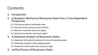
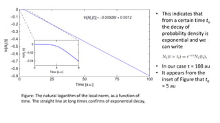
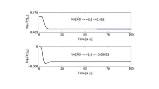
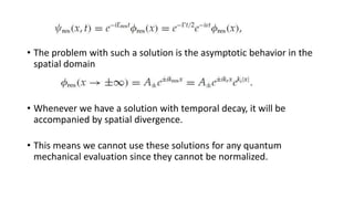
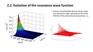
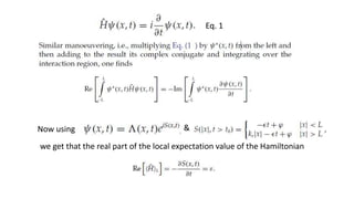
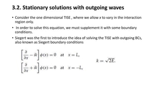
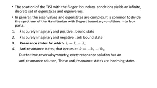
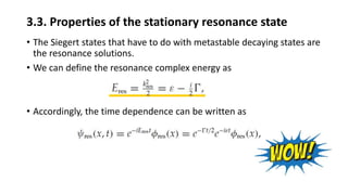
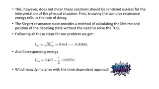
1. The document discusses quantum mechanical resonance states from both a time-dependent and stationary perspective. 2. From the time-dependent view, a resonance state begins as a bound state that decays exponentially over time within the interaction region, while developing an outgoing wavefront outside the region. 3. The stationary analysis models resonance states as solutions to the time-independent Schrodinger equation with outgoing boundary conditions, yielding complex energies whose imaginary parts determine lifetimes.

1. Quantum Mechanical
Resonance
A First Glance into
the Behavior of Unstable States#
Sumit Kale
Department of Chemistry
Indian Institute of Technology, Guwahati, Assam, India
# Shachar Klaiman and Ido Gilary , January 2012 ,Advances in Quantum Chemistry 63:1-31

2. Contents
1. Introduction
2. A Quantum Mechanical Resonance State from a Time-Dependent
Perspective
2.1. From bound state to metastable state
2.2. Evolution of the resonance wave function
2.3. Dynamics inside the interaction region
2.4. Dynamics outside the interaction region
3. A Stationary Analysis of Resonance States
3.1. Expansion of localized functions in terms of scattering states
3.2. Stationary solutions with outgoing waves
3.3. Properties of the stationary resonance state
4. Unified Picture of Resonance States

3. Introduction
• The word resonance is a very widespread term in the scientific world. Common
uses range from being in a or on resonance to resonance poles and peaks.
• This can lead to some confusion and ambiguity when different definitions are
evoked
• Here, we wish to explore the meaning of this term attributed to unstable states in
quantum mechanics
Quantum Mechanical System
Bound State Solutions Continuum State Solutions

4. • Quantization facilitates the understanding of quantum phenomena related to
bound states since one can often relate the desired phenomenon with the
occupation of only a few well-defined states.
• In the continuum, we are forced to use wave packets rather than a single
eigenstate to describe quantum particles.
• Wave packets are built by integrating over a continuous range of energy
eigenstates to create localized wave functions.
• Therefore, when describing phenomena that require the continuous part of the
spectrum, it becomes increasingly difficult to correlate an observed effect with a
single eigenstate of the TISE.

5. • Many physical situations allow for a simpler approach based on
resonance states. Resonance states are quantized solutions of
the TISE, which correspond to unstable quantum states, i.e.,
states with a finite lifetime.
• Therefore, describing a continuum wave packet using such
resonance states would circumvent one of the biggest difficulties
in the continuum
• The inability to associate the physical phenomenon with a finite
number of physical states.
• Most importantly we would be looking at a “stationary nature”
of the time-dependent dynamics.

6. 2. A Quantum Mechanical Resonance State from a Time-
Dependent Perspective
• 2.1. From bound state to metastable state
• The one-dimensional potential is
depicted for two different choices
of :
(a) α = 0
(b) α = 0.05
• The following parameters are the
same for both potentials: Vo=1
β =1

7. • A general time-dependent solution can be written as
• Perturbing the bound system such that the potential is changed and now α =
0.05.
• The new potential does not support any bound states, and the entire spectrum is
continuous.
• Particle previously inhabiting the bound state wave function Ψo is no longer in a
stationary state. The previous eigenstate is now a wave packet, a superposition of
the eigenstates of the perturbed Hamiltonian

8. 2.2. Evolution of the resonance wave function
• Clearly, the probability density decays inside
the interaction region pointing out the finite
lifetime of the previously bound particle, i.e.,

9. The phase drops linearly with time. In accordance with the snapshots. It
also shows the phase growing linearly with the position outside the
interaction region and remaining constant within it.

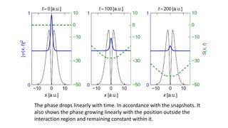
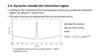
10. • The above evidences suggests the
following general form for 𝑆 𝑥, 𝑡
• In our case L = 5 au
• The rate of change of the local phase
obtained from a linear regression on
the outer part is
𝑑𝑠
𝑑𝑥
= 𝐾𝑟 = 0.965 [𝑎𝑢]
• The rate of change of the phase in time
is
𝑑𝑠
𝑑𝑡
= − ε = − 0.465 [𝑎𝑢]
• To sum-up Inside the interaction region, we have the phase behavior of a
bound state, whereas outside we have the behavior of a continuum state 

11. 2.3. Dynamics inside the interaction region
• The probability density in the interaction region decays exponentially.
• This can be verified by calculating the norm inside the interaction
region, which is given by

12. Figure: The natural logarithm of the local norm, as a function of
time. The straight line at long times confirms of exponential decay,
• This indicates that
from a certain time to
the decay of
probability density is
exponential and we
can write
• In our case τ = 108 au
• It appears from the
inset of Figure that t0
= 5 au

13. • Calculating the local expectation value of the Hamiltonian inside the
interaction region
Consider Ψ 𝑥, 𝑡 a solution of the TDSE satisfying
Eq. 1

14. Integrating from -L to +L, we find that
Eq. 2
we can conclude that for sufficiently long times

15. Eq. 1
Now using &
we get that the real part of the local expectation value of the Hamiltonian

17. • Therefore, the local expectation value of the Hamiltonian reads
• So wave function within the interaction region after t > t0 can be given by
• The wave packet inside the interaction region and at longer time behaves much
like a stationary state with a complex energy.
• Hopefully, we are now comfortable to state that a quantum mechanical
resonance state is an exponentially decaying metastable state of the system
localized in the interaction region with a finite lifetime and positioned at an
energy ε .

18. 2.4. Dynamics outside the interaction region
• Looking on the amplitude of the evolving wave packet just outside the interaction
region, we observe a “wave front.”
• This wave front has an exponential form as can be observed as
Outside the barriers
we can more or less
write
The probability density of the wave packet at time t = 200 on
a logarithmic scale.

19. 3. A Stationary Analysis of Resonance States
• Resonance states can be described using the solution of the TDSE by analyzing
the evolution of a wave packet.
• This kind of analysis is, however, usually difficult and time consuming as the wave
packet needs to be propagated to large times, which is often challenging
numerically.
• We observed that at the sufficient longer-time the wave packet in the interaction
region resembles that of a stationary state with a complex energy.
• Can we calculate this stationary state without the need to solve
the TDSE,i.e., without propagating the wave packet ?

20. 3.1. Expansion of localized functions in terms of
scattering states
• Consider the stationary solutions of the TISE for the perturbed potential.
Explicitly the solution of the following eigenvalue equation:
• The bound state of the unperturbed system becomes a superposition of the
eigenstates of the perturbed system (α = 0.05)
• We may attempt an analysis of the evolving wave packet based on the
eigenstates of the new problem.

21. • Since the potential is now unbound, it supports only a continuum of scattering
states φE. Fig. portrays several continuum eigenstates of the Hamiltonian.
The probability density of several continuum eigenstates of the
Hamiltonian plotted on the baseline of their corresponding energy.

22. • The wave packet will contain contributions from two “groups” of continuum
eigenstates, which will depend on the expansion coefficients C(E) given and can
now be separated to

23. 3.2. Stationary solutions with outgoing waves
• Consider the one dimensional TISE , where we allow x to vary in the interaction
region only.
• In order to solve this equation, we must supplement it with some boundary
conditions.
• Siegert was the first to introduce the idea of solving the TISE with outgoing BCs,
also known as Siegert boundary conditions

24. • The solution of the TISE with the Siegert boundary conditions yields an infinite,
discrete set of eigenstates and eigenvalues.
• In general, the eigenvalues and eigenstates are complex. It is common to divide
the spectrum of the Hamiltonian with Siegert boundary conditions into four
parts:
1. k is purely imaginary and positive : bound state
2. k is purely imaginary and negative : anti bound state
3. Resonance states for which
4. Anti-resonance states, that occurs at
Due to time-reversal symmetry, every resonance solution has an
anti-resonance solution, These anti-resonance states are incoming states

25. 3.3. Properties of the stationary resonance state
• The Siegert states that have to do with metastable decaying states are
the resonance solutions.
• We can define the resonance complex energy as
• Accordingly, the time dependence can be written as

26. • The problem with such a solution is the asymptotic behavior in the
spatial domain
• Whenever we have a solution with temporal decay, it will be
accompanied by spatial divergence.
• This means we cannot use these solutions for any quantum
mechanical evaluation since they cannot be normalized.

27. • This, however, does not mean these solutions should be rendered useless for the
interpretation of the physical situation. First, knowing the complex resonance
energy tells us the rate of decay.
• The Siegert resonance state provides a method of calculating the lifetime and
position of the decaying state without the need to solve the TDSE
• Following all these steps for our problem we got :
• And Corresponding energy
• Which exactly matches with the time dependent approach

28. 4. Unified Picture of Resonance States
• In the previous sections, we have seen that a resonance can be
described through both a time-dependent approach and a time-
independent approach.
• The goal of this section is to create a unified picture that joins both
methodologies

29. Lets recap the properties of a wave packet populating a resonant state
we observed in Section 2:
1. After some initial rearrangement time, a bound-like wave function
is obtained in the interaction region.
2. Outside the interaction region, one observes escaping particles with
constant velocity.
3. The local expectation of the energy inside the interaction region is
complex. This complex value saturates to a constant value as time
evolves
4. Outside the interaction region, the probability density seems to
increase exponentially in space.

30. Lets recap the properties of a stationary analysis of a resonant state we
observed in Section 3:
• The asymptotic behavior of a resonance state is of outgoing waves,
i.e.
• The energy of a resonance state is complex. This is the result of the
BCs that render the Hamiltonian non-Hermitian
• The time-dependent resonance wave function decays in time
because of the negative imaginary part of the complex energy.

31. • The joint properties of the two approaches above stem from the fact
that the time-dependent resonance ansatz of Section 2 is completely
reproduced by the stationary resonance solution of the TISE of
Section 3
• That’s what our Objective was “stationary” nature of time dependent
dynamics