Quantile Based Reliability Analysis 1st Edition N. Unnikrishnan Nair
Quantile Based Reliability Analysis 1st Edition N. Unnikrishnan Nair
Quantile Based Reliability Analysis 1st Edition N. Unnikrishnan Nair
Quantile Based Reliability Analysis 1st Edition N. Unnikrishnan Nair
Quantile Based Reliability Analysis 1st Edition N. Unnikrishnan Nair
1.
Quantile Based ReliabilityAnalysis 1st Edition
N. Unnikrishnan Nair pdf download
https://ebookgate.com/product/quantile-based-reliability-
analysis-1st-edition-n-unnikrishnan-nair/
Get the full ebook with Bonus Features for a Better Reading Experience on ebookgate.com
2.
Instant digital products(PDF, ePub, MOBI) available
Download now and explore formats that suit you...
Advances in Reliability 1st Edition N. Balakrishnan
https://ebookgate.com/product/advances-in-reliability-1st-edition-n-
balakrishnan/
ebookgate.com
Safety Reliability and Risk Analysis Theory Methods and
Applications 3rd Edition 4 Volumes Sebastián Martorell
https://ebookgate.com/product/safety-reliability-and-risk-analysis-
theory-methods-and-applications-3rd-edition-4-volumes-sebastian-
martorell/
ebookgate.com
Safety Reliability and Risk Analysis Beyond the Horizon
R.D.J.M. Steenbergen
https://ebookgate.com/product/safety-reliability-and-risk-analysis-
beyond-the-horizon-r-d-j-m-steenbergen/
ebookgate.com
Quantile Regression Theory and Applications 1st Edition
Cristina Davino
https://ebookgate.com/product/quantile-regression-theory-and-
applications-1st-edition-cristina-davino/
ebookgate.com
3.
Vascular Biology Protocols1st Edition Nair Sreejayan
https://ebookgate.com/product/vascular-biology-protocols-1st-edition-
nair-sreejayan/
ebookgate.com
Advances in Survival Analysis N. Balakrishnan
https://ebookgate.com/product/advances-in-survival-analysis-n-
balakrishnan/
ebookgate.com
World Clinics Diabetology Type 2 Diabetes Mellitus 1st
Edition Ranjit Unnikrishnan
https://ebookgate.com/product/world-clinics-diabetology-
type-2-diabetes-mellitus-1st-edition-ranjit-unnikrishnan/
ebookgate.com
Computer Ethics A Case based Approach 1st Edition Robert
N. Barger
https://ebookgate.com/product/computer-ethics-a-case-based-
approach-1st-edition-robert-n-barger/
ebookgate.com
Evidence based Management of Lipid Disorders 1st Edition
Maud N. Vissers
https://ebookgate.com/product/evidence-based-management-of-lipid-
disorders-1st-edition-maud-n-vissers/
ebookgate.com
5.
Statistics for Industryand Technology
Quantile-
Based
Reliability
Analysis
N. Unnikrishnan Nair
P.G. Sankaran
N. Balakrishnan
7.
Statistics for Industryand Technology
Series Editor
N. Balakrishnan
McMaster University
Hamilton, ON
Canada
Editorial Advisory Board
Max Engelhardt
EG&G Idaho, Inc.
Idaho Falls, ID, USA
Harry F. Martz
Los Alamos National Laboratory
Los Alamos, NM, USA
Gary C. McDonald
NAO Research & Development Center
Warren, MI, USA
Kazuyuki Suzuki
University of Electro Communications
Chofu-shi, Tokyo
Japan
For further volumes:
http://www.springer.com/series/4982
8.
N. Unnikrishnan Nair• P.G. Sankaran
N. Balakrishnan
Quantile-Based Reliability
Analysis
To Jamuna, Anoopand Arun
NUN
To Sandhya, Revathi and Nandana
PGS
To Julia, Sarah and Colleen
NB
12.
Foreword
Quantile functions area fundamental, and often the most natural, way of rep-
resenting probability distributions and data samples. In much of environmental
science, finance, and risk management, there is a need to know the event magnitude
corresponding to a given return period or exceedance probability, and the quantile
function provides the most direct expression of the solution. The book Statistical
Modelling with Quantile Functions by Warren Gilchrist provides an extensive
survey of quantile-based methods of inference for complete distributions.
Reliability analysis is another field in which quantile-based methods are partic-
ularly useful. In many applications one must deal with censored data and truncated
distributions, and concepts such as hazard rate and residual life become important.
Quantile-based methods need some extensions to deal with these issues, and the
present book goes beyond Prof. Gilchrist’s and provides a thorough grounding in
the relevant theory and practical methods for reliability analysis.
I have been fortunate in having been able for over 20 years to develop a theory
of L-moments, statistics that are simple and effective inferences about probability
distributions. Although not restricted to quantile-based inference, L-moments lend
themselves well to quantile methods since many of the key results regarding
L-moments are most conveniently expressed in terms of the quantile function.
As with quantile methods generally, an L-moment-based approach to reliability
analysis has not been developed in detail. In this book the authors have made
significant progress, and in particular the development of L-moment methods for
residual life analysis is a major step forward. I congratulate the authors on their
achievements, and I invite the readers of this book to enjoy a survey of material that
is rich in both theoretical depth and practical utility.
Yorktown Heights, NY J.R.M. Hosking
vii
14.
Preface
Reliability theory hastaken rapid strides in the last four decades to become
an independent discipline that influences our daily lives and schedules through
our dependence on good and reliable functioning of devices and systems that
we constantly use. The extensive literature on reliability theory, along with its
applications, is scattered over various disciplines including statistics, engineering,
applied probability, demography, economics, medicine, survival analysis, insurance
and public policy. Life distributions specified by their distribution functions and
various concepts and characteristics derived from it occupy a big portion of
reliability analysis. Although quantile functions also represent life distributions and
would facilitate one to carry out all the principal functions enjoyed by distribution
functions in the existing theory and practice, this feature is neither fully appreciated
nor exploited. The objective of this book is to attempt a systematic study of various
aspects of reliability analysis with the aid of quantile functions, so as to provide
alternative methodologies, new models and inferential results that are sometimes
difficult to accomplish through the conventional approach.
Due to the stated objective, the material presented in this book is loaded with a
quantile flavour. However, all through the discussion, we first present a concept or
methodology in terms of the conventional approach and only introduce the quantile-
based counterpart. This will enable the reader to transfer the methodology from one
form to the other and to choose the one that fits his/her taste and need. Being an
introductory text in quantile-based reliability methods, there is scope for further
improvements and extensions of the results discussed here.
The book is biased towards the mathematical theory, with examples intended to
clarify various notions and applications to real data being limited to demonstrate the
utility of quantile functions. For those with interest in practical aspects of quantile-
based model building, relevant tools and descriptive data analysis, the book by
Gilchrist would provide a valuable guidance.
This book is organized into nine chapters. Chapter 1 deals with the definition,
properties and various descriptive measures based on the quantile functions. Various
reliability concepts like hazard rate, and mean residual life, in the conventional form
as well as their quantile equivalents, are discussed in Chap. 2. This is followed, in
Chap. 3, by a detailed presentation of the distributional and reliability aspects of
ix
15.
x Preface
quantile functionmodels along with some applications to real data. Different ageing
concepts in quantile versions are described in Chap. 4. Total time on test transforms,
an essentially quantile-based notion, is detailed in Chap.5. As alternatives to the
conventional moments, the L-moments and partial moments in relation to residual
life are presented. In Chap. 6, the definitions, properties and characterizations of
these concepts are explained along with their use in inferential methods. Bathtub
hazard models are considered in Chap. 7 along with their quantile counterparts and
some new quantile functions that exhibit nonmonotone hazard quantile functions.
The definitions and properties of various stochastic orders encountered in reliability
theory are described in Chap. 8. Finally, Chap. 9 deals with various methods of
estimation and modelling problems. A more detailed account of the contents of
each chapter is provided in the Abstract at the beginning of each chapter.
Within the space available for this book, it has not been possible to include all
the topics pertinent to reliability analysis. Likewise, the work of many authors who
have contributed to these topics, as well as to those in the text, could not be included
in the book. Our sincere apologies for these shortcomings. Any suggestion for the
improvement in the contents and/or indication of possible errors in the book are
wholeheartedly welcomed.
Finally, we wish to thank Sanjai Varma, Vinesh Kumar and K. P. Sasidharan for
their contributions to the cause of this work. We are grateful to the colleagues in the
Department of Statistics and Administration of the Cochin University of Science
and Technology. Our sincere thanks also go to Ms. Debbie Iscoe for her help with
the final typesetting and production of the volume.
Finally, we would like to state formally that this project was catalysed and
supported by the Department of Science and Technology, Government of India,
under its Utilisation of Scientific Expertise of Retired Scientist Scheme.
Cochin, India N. Unnikrishnan Nair
Cochin, India P.G. Sankaran
Hamilton, ON, Canada N. Balakrishnan
16.
Contents
1 Quantile Functions...........................................................1
1.1 Introduction ............................................................ 1
1.2 Definitions and Properties ............................................. 3
1.3 Quantile Functions of Life Distributions ............................. 9
1.4 Descriptive Quantile Measures........................................ 9
1.5 Order Statistics......................................................... 16
1.6 Moments ............................................................... 20
1.7 Diagrammatic Representations........................................ 26
2 Quantile-Based Reliability Concepts ...................................... 29
2.1 Concepts Based on Distribution Functions ........................... 29
2.1.1 Hazard Rate Function ......................................... 30
2.1.2 Mean Residual Life Function ................................. 32
2.1.3 Variance Residual Life Function.............................. 36
2.1.4 Percentile Residual Life Function ............................ 39
2.2 Reliability Functions in Reversed Time .............................. 41
2.2.1 Reversed Hazard Rate ......................................... 41
2.2.2 Reversed Mean Residual Life................................. 43
2.2.3 Some Other Functions ........................................ 45
2.3 Hazard Quantile Function ............................................. 46
2.4 Mean Residual Quantile Function .................................... 51
2.5 Residual Variance Quantile Function ................................. 54
2.6 Other Quantile Functions.............................................. 56
3 Quantile Function Models .................................................. 59
3.1 Introduction ............................................................ 59
3.2 Lambda Distributions.................................................. 60
3.2.1 Generalized Lambda Distribution ............................ 62
3.2.2 Generalized Tukey Lambda Family .......................... 75
3.2.3 van Staden–Loots Model...................................... 81
3.2.4 Five-Parameter Lambda Family .............................. 85
3.3 Power-Pareto Distribution ............................................. 88
xi
17.
xii Contents
3.4 Govindarajulu’sDistribution .......................................... 93
3.5 Generalized Weibull Family........................................... 98
3.6 Applications to Lifetime Data......................................... 100
4 Ageing Concepts ............................................................. 105
4.1 Introduction ............................................................ 105
4.2 Reliability Operations ................................................. 107
4.2.1 Coherent Systems ............................................. 107
4.2.2 Convolution.................................................... 108
4.2.3 Mixture......................................................... 108
4.2.4 Shock Models ................................................. 109
4.2.5 Equilibrium Distributions ..................................... 110
4.3 Classes Based on Hazard Quantile Function ......................... 113
4.3.1 Monotone Hazard Rate Classes............................... 113
4.3.2 Increasing Hazard Rate(2) .................................... 122
4.3.3 New Better Than Used in Hazard Rate....................... 123
4.3.4 Stochastically Increasing Hazard Rates ...................... 125
4.3.5 Increasing Hazard Rate Average.............................. 126
4.3.6 Decreasing Mean Time to Failure ............................ 128
4.4 Classes Based on Residual Quantile Function ....................... 130
4.4.1 Decreasing Mean Residual Life Class........................ 130
4.4.2 Used Better Than Aged Class................................. 134
4.4.3 Decreasing Variance Residual Life ........................... 136
4.4.4 Decreasing Percentile Residual Life Functions .............. 139
4.5 Concepts Based on Survival Functions ............................... 140
4.5.1 New Better Than Used ........................................ 140
4.5.2 New Better Than Used in Convex Order ..................... 146
4.5.3 New Better Than Used in Expectation ....................... 149
4.5.4 Harmonically New Better Than Used ........................ 151
4.5.5 L and M Classes............................................. 153
4.5.6 Renewal Ageing Notions...................................... 154
4.6 Classes Based on Concepts in Reversed Time ....................... 156
4.7 Applications............................................................ 158
4.7.1 Analysis of Quantile Functions ............................... 158
4.7.2 Relative Ageing ............................................... 163
5 Total Time on Test Transforms ............................................. 167
5.1 Introduction ............................................................ 168
5.2 Definitions and Properties ............................................. 168
5.3 Relationships with Other Curves...................................... 174
5.4 Characterizations of Ageing Concepts................................ 182
5.5 Some Generalizations ................................................. 185
5.6 Characterizations of Distributions .................................... 191
5.7 Some Applications..................................................... 193
18.
Contents xiii
6 L-Momentsof Residual Life and Partial Moments....................... 199
6.1 Introduction ............................................................ 200
6.2 Definition and Properties of L-Moments of Residual Life........... 201
6.3 L-Moments of Reversed Residual Life ............................... 211
6.4 Characterizations ...................................................... 213
6.5 Ageing Properties...................................................... 224
6.6 Partial Moments ....................................................... 225
6.7 Some Applications..................................................... 230
7 Nonmonotone Hazard Quantile Functions................................ 235
7.1 Introduction ............................................................ 236
7.2 Two-Parameter BT and UBT Hazard Functions ..................... 236
7.3 Three-Parameter BT and UBT Models ............................... 248
7.4 More Flexible Hazard Rate Functions ................................ 261
7.5 Some General Methods of Construction.............................. 267
7.6 Quantile Function Models............................................. 269
7.6.1 Bathtub Hazard Quantile Functions Using Total
Time on Test Transforms...................................... 269
7.6.2 Models Using Properties of Score Function ................. 273
8 Stochastic Orders in Reliability ............................................ 281
8.1 Introduction ............................................................ 281
8.2 Usual Stochastic Order ................................................ 283
8.3 Hazard Rate Order ..................................................... 287
8.4 Mean Residual Life Order............................................. 291
8.5 Renewal and Harmonic Renewal Mean Residual Life Orders ...... 298
8.6 Variance Residual Life Order ......................................... 302
8.7 Percentile Residual Life Order ........................................ 303
8.8 Stochastic Order by Functions in Reversed Time .................... 306
8.8.1 Reversed Hazard Rate Order.................................. 306
8.8.2 Other Orders in Reversed Time............................... 308
8.9 Total Time on Test Transform Order.................................. 311
8.10 Stochastic Orders Based on Ageing Criteria ......................... 314
8.11 MTTF Order ........................................................... 320
8.12 Some Applications..................................................... 322
9 Estimation and Modelling................................................... 327
9.1 Introduction ............................................................ 327
9.2 Method of Percentiles ................................................. 328
9.3 Method of Moments ................................................... 334
9.3.1 Conventional Moments ....................................... 334
9.3.2 L-Moments .................................................... 336
9.3.3 Probability Weighted Moments............................... 341
9.4 Method of Maximum Likelihood ..................................... 344
9.5 Estimation of the Quantile Density Function......................... 346
9.6 Estimation of the Hazard Quantile Function ......................... 350
19.
xiv Contents
9.7 Estimationof Percentile Residual Life ............................... 352
9.8 Modelling Failure Time Data ......................................... 355
9.9 Model Identification ................................................... 356
9.10 Model Fitting and Validation.......................................... 358
References......................................................................... 361
Index ............................................................................... 385
Author Index...................................................................... 391
20.
List of Figures
Fig.1.1 Q-Q plot for Example 1.12............................................ 27
Fig. 1.2 Box plot for the data given in Example 1.12 ......................... 28
Fig. 3.1 Density plots of the generalized lambda distribution
(Ramberg and Schmeiser [503] model) for different
choices of (λ1,λ2,λ3,λ4). (a) (1,0.2,0.13,0.13);
(b) (1,0.6,1.5,-1.5); (c) (1,0.6,1.75,1.2); (d)
(1,0.2,0.13,0.013); (e) (1,0.2,0.0013,0.13); (f) (1,1,0.5,4) ........... 65
Fig. 3.2 Density plots of the GLD (Freimer et al. model) for
different choices of (λ1,λ2,λ3,λ4). (a) (2,1,2,0.5);
(b) (2,1,0.5,2); (c) (2,1,0.5,0.5); (d) (3,1,1.5,2.5); (e)
(3,1,1.5,1.6,); (f) (1,1,2,0.1); (g) (5,1,0.1,2) .......................... 77
Fig. 3.3 Density plots of the GLD proposed by van Staden and
Loots [572] for varying (λ1,λ2,λ3,λ4). (a) (1,1,0.5,2);
(b) (2,1,0.5,3); (c) (3,2,0.25,0.5); (d) (1,2,0.1,−1)................... 84
Fig. 3.4 Density plots of the five-parameter GLD for different
choices of (λ1,λ2,λ3,λ4,λ5). (q) (1,1,0,10,10); (b)
(1,1,0,2,2); (c) (1,1,0.5,-0.6,-0.5); (d) (1,1,-0.5,-0.6,
-0.5); (e) (1,1,0.5,0.5,5) ............................................... 86
Fig. 3.5 Density plots of power-Pareto distribution for some
choices of (C,λ1,λ2). (a) (1,0.5,0.01); (b) (1,1,0.2); (c)
(1,0.2,0.1); (d) (1,0.1,1); (e) (1,0.5,0.001); (f) (1,2,0.001) .......... 89
Fig. 3.6 Density plots of Govindarajulu’s distribution for some
choices of β. (a) β = 3; (b) β = 0.5; (c) β = 2...................... 94
Fig. 3.7 Q-Q plot for the data on lifetimes of aluminum coupons............ 101
Fig. 3.8 Q-Q plot for the data on times to first failure of electric carts....... 102
Fig. 3.9 Q-Q plot for the data on failure times of devices using
Govindarajulu’s model ................................................ 102
Fig. 4.1 Implications among different ageing concepts ....................... 157
Fig. 4.2 Plots of hazard quantile function when (1) β = 0.1,
σ = 1 and (2) β = 2, σ = 1 for Govindarajalu’s distribution ....... 160
xv
21.
xvi List ofFigures
Fig. 4.3 Plots of hazard quantile function when (1) C = 0.1,
λ1 = 0.5, λ2 = 0.01; (2) C = 0.5, λ1 = 2, λ2 = 0.01;
(3) C = 0.01, λ1 = 2, λ2 = 0.5; (4) C = 0.01, λ1 = 0.5,
λ2 = 0.5, for the power-Pareto distribution .......................... 160
Fig. 4.4 Plots of hazard quantile function when (1) λ1 = 0,
λ2 = 100, λ3 = −0.5, λ4 = −0.1; (2) λ1 = 0, λ2 = 500,
λ3 = 3, λ4 = 2; (3) λ1 = 0, λ2 = 2, λ3 = 10, λ4 = 5;
(4) λ1 = 0, λ2 = 100, λ3 = 2, λ4 = 0.5; (5) λ1 = 0,
λ2 = 250, λ3 = 2, λ4 = 0.001, for the generalized Tukey
lambda distribution .................................................... 161
Fig. 4.5 Plots of hazard quantile function when (1) λ1 = 1,
λ2 = 100, λ3 = 0.05, λ4 = 0.5; (2) λ1 = 0, λ2 = −1000,
λ3 = 0, λ4 = −2; (3) λ1 = 1, λ2 = 10, λ3 = 2, λ4 = 0;
(4) λ1 = 0, λ2 = −1000, λ3 = −2, λ4 = −1, for the
generalized lambda distribution....................................... 162
Fig. 4.6 Plots of hazard quantile function when (1) λ1 = 0,
λ2 = 0.01, λ3 = 0.5, λ4 = −2; (2) λ1 = 0, λ2 = 100,
λ3 = 0.5, λ4 = 10; (3) λ1 = 0, λ2 = 1, λ3 = 0.6,
λ4 = 0.5; (4) λ1 = 0, λ2 = 0.1, λ3 = 1, λ4 = −5, for the
van Staden–Loots model .............................................. 163
Fig. 6.1 Plot of M(u) and l2(u) for the data on lifetimes of
aluminum coupons .................................................... 207
Fig. 6.2 Plot of M(u) and l2(u) for the data on failure times of a
set of refrigerators ..................................................... 208
Fig. 6.3 Plot of M(u) and l2(u) for the data on failure times of
electric carts............................................................ 209
22.
Acronyms
X,Y,Z Continuous randomvariables
F(x) Distribution function of X
Q(u) Quantile function corresponding to F(x)
f(x) Probability density function of X
q(u) Quantile density function
Xt Residual life at age t
F̄(x) Survival function of X
F̄t(x) Survival function of Xt
M Median
S Galton’s coefficient of skewness
T Moors’ measure of kurtosis
Δ Gini’s mean difference
Xr:n rth order statistic in a sample of size n
Lr rth L-moment
τ2 L-coefficient of variation
τ3 L-coefficient of skewness
τ4 L-coefficient of kurtosis
h(x) Hazard rate of X
H(u) Hazard quantile function of X
m(x) Mean residual life function
M(u) Mean residual quantile function
σ2(x) Variance residual life function
V(u) Variance residual quantile function
pα(x) Percentile residual life function
Pα(u) Percentile residual quantile function
λ(x) Reversed hazard rate function
Λ(u) Reversed hazard quantile function
r(x) Reversed mean residual life
R(u) Reversed mean residual quantile function
v(x) Reversed variance residual life function
xvii
23.
xviii Acronyms
D(u) Reversedvariance quantile function
qα(x) Reversed percentile residual life function
σ2 Variance of X
μr rth central moment of X
lr rth sample Λ-moment
J(u) Score function
τ(·) Total time on test statistic
Fn(x) Empirical distribution function
T(u) Total time on test transform
φ(u) Scaled total time on test transform
L(u) Lorenz curve
G Gini index
B(u) Bonferroni curve
K(u) Leimkuhler curve
Tn(u) Total time on test transform of order n
Lr(t) rth L-moment of X|(X > t)
lr(u) Quantile version of Lr(t)
Br(t) rth L-moment of X|(X ≤ t)
θr(u) Quantile version of Br(t)
Pr(u) Upper partial moment of order r
P∗
r (u) Lower partial moment of order r
Qn(p) Empirical quantile function
ξp Sample quantile
Mp,rs Probability weighted moments
≤st Usual stochastic order
≤hr Hazard rate order
≤mrl Mean residual life order
≤rmrl Renewal mean residual life order
≤hrmrl Harmonic renewal mean residual life order
≤vrl Variance residual life order
≤prl−α Percentile residual life order
≤rh Reversed hazard rate order
≤MIT Mean inactivity time order
≤VIT Variance inactivity time order
≤TTT Total time on test transform order
≤c Convex transform order
≤∗ Star order
≤su Super additive order
≤NBUHR New better than used in hazard rate order
≤DMRL Decreasing mean residual life order
≤NBUE New better than used in expectation order
≤MTTF Mean time to failure order
BT (UBT) Bathtub-shaped hazard rate (upside-down bathtub-shaped hazard
rate)
24.
Acronyms xix
DCSS Decreasingcumulative survival class
DHRA Decreasing hazard rate average
DMERL Decreasing median residual life
DMRL Decreasing mean residual life
DMRLHA Decreasing mean residual life in harmonic average
DMTTF Decreasing mean time to failure
DPRL Decreasing percentile residual life
DRMRL Decreasing renewal mean residual life
DVRL Decreasing variance residual life
GIMRL Generalized increasing mean residual life
HNBUE Harmonically new better than used
HNWUE Harmonically new worse than used
HRNBUE Harmonically renewal new better than used in expectation
HUBAE Harmonically used better than aged
ICSS Increasing cumulative survival class
IHR (2) Increasing hazard rate of order 2
IHR (DHR) Increasing hazard rate (decreasing hazard rate)
IHRA Increasing hazard rate average
IMERL Increasing median residual life
IMIT Increasing mean inactivity time
IMRL Increasing mean residual life
IPRL Increasing percentile residual life
IQR Interquartile range
IRMRL Increasing renewal mean residual life
IVRL Increasing variance residual life
NBRU New better than renewal used
NBU New better than used
NBUC New better than used in convex order
NBUCA New better than used in convex average
NBUE New better than used in expectation
NBUHR New better than used in hazard rate
NBUHRA New better than used in hazard rate average
NBUL New better than used in Laplace order
NDMRL Net decreasing mean residual life
NWRU New worse than renewal used
NWU New worse than used
NWUC New worse than used in convex order
NWUE New worse than used in expectation
NWUHR New worse than used in hazard rate
NWUHRA New worse than used in hazard rate average
NWUL New worse than used in Laplace order
RNBRU Renewal new is better than renewal used
RNBRUE Renewal new is better than renewal used in expectation
RNBU Renewal new is better than used
RNBUE Renewal new is better than used in expectation
25.
xx Acronyms
RNWU Renewalnew is worse than used
SIHR Stochastically increasing hazard rate
SNBU Stochastically new better than used
TTT Total time on test transform
UBA Used better than aged
UBAE Used better than aged in expectation
UWA Used worse than aged
UWAE Used worse than aged in expectation
2 1 QuantileFunctions
an appropriate choice of the domain of observations, a better understanding of a
chance phenomenon can be achieved by the use of quantile functions, is fast gaining
acceptance.
Historically, many facts about the potential of quantiles in data analysis were
known even before the nineteenth century. It appears that the Belgian sociologist
Quetelet [499] initiated the use of quantiles in statistical analysis in the form of the
present day inter-quantile range. A formal representation of a distribution through
a quantile function was introduced by Galton (1822–1911) [206] who also initiated
the ordering of observations along with the concepts of median, quartiles and
interquartile range. Subsequently, the research on quantiles was directed towards
estimation problems with the aid of sample quantiles, their large sample behaviour
and limiting distributions (Galton [207, 208]). A major development in portraying
quantile functions to represent distributions is the work of Hastings et al. [264], who
introduced a family of distributions by a quantile function. This was refined later
by Tukey [568]. The symmetric distribution of Tukey [568] and his articulation
of exploratory data analysis sparked considerable interest in quantile functional
forms that continues till date. Various aspects of the Tukey family and general-
izations thereto were studied by a number of authors including Hogben [273],
Shapiro and Wilk [536], Filliben [197], Joiner and Rosenblatt [304], Ramberg
and Schmeiser [504], Ramberg [501], Ramberg et al. [502], MacGillivray [407],
Freimer et al. [203], Gilchrist [215] and Tarsitano [563]. We will discuss all these
models in Chap. 3. Another turning point in the development of quantile functions
is the seminal paper by Parzen [484], in which he emphasized the description
of a distribution in terms of the quantile function and its role in data modelling.
Parzen [485–487] exhibits a sequential development of the theory and application
of quantile functions in different areas and also as a tool in unification of various
approaches.
Quantile functions have several interesting properties that are not shared by
distributions, which makes it more convenient for analysis. For example, the sum
of two quantile functions is again a quantile function. There are explicit general dis-
tribution forms for the quantile function of order statistics. In Sect. 1.2, we mention
these and some other properties. Moreover, random numbers from any distribution
can be generated using appropriate quantile functions, a purpose for which lambda
distributions were originally conceived. The moments in different forms such as raw,
central, absolute and factorial have been used effectively in specifying the model,
describing the basic characteristics of distributions, and in inferential procedures.
Some of the methods of estimation like least squares, maximum likelihood and
method of moments often provide estimators and/or their standard errors in terms
of moments. Outliers have a significant effect on the estimates so derived. For
example, in the case of samples from the normal distribution, all the above methods
give sample mean as the estimate of the population mean, whose values change
significantly in the presence of an outlying observation. Asymptotic efficiency of the
sample moments is rather poor for heavy tailed distributions since the asymptotic
variances are mainly in terms of higher order moments that tend to be large in this
case. In reliability analysis, a single long-term survivor can have a marked effect
28.
1.2 Definitions andProperties 3
on mean life, especially in the case of heavy tailed models which are commonly
encountered for lifetime data. In such cases, quantile-based estimates are generally
found to be more precise and robust against outliers. Another advantage in choosing
quantiles is that in life testing experiments, one need not wait until the failure of
all the items on test, but just a portion of them for proposing useful estimates.
Thus, there is a case for adopting quantile functions as models of lifetime and base
their analysis with the aid of functions derived from them. Many other facets of
the quantile approach will be more explicit in the sequel in the form of alternative
methodology, new opportunities and unique cases where there are no corresponding
results if one adopts the distribution function approach.
1.2 Definitions and Properties
In this section, we define the quantile function and discuss some of its general
properties. The random variable considered here has the real line as its support, but
the results are valid for lifetime random variables which take on only non-negative
values.
Definition 1.1. Let X be a real valued continuous random variable with distribution
function F(x) which is continuous from the right. Then, the quantile function Q(u)
of X is defined as
Q(u) = F−1
(u) = inf{x : F(x) ≥ u}, 0 ≤ u ≤ 1. (1.1)
For every −∞ < x < ∞ and 0 < u < 1, we have
F(x) ≥ u if and only if Q(u) ≤ x.
Thus, if there exists an x such that F(x) = u, then F(Q(u)) = u and Q(u) is the
smallest value of x satisfying F(x) = u. Further, if F(x) is continuous and strictly
increasing, Q(u) is the unique value x such that F(x) = u, and so by solving the
equation F(x) = u, we can find x in terms of u which is the quantile function of X.
Most of the distributions we consider in this work are of this form and nature.
Definition 1.2. If f(x) is the probability density function of X, then f(Q(u)) is
called the density quantile function. The derivative of Q(u), i.e.,
q(u) = Q
(u),
is known as the quantile density function of X. By differentiating F(Q(u)) = u, we
find
q(u)f(Q(u)) = 1. (1.2)
29.
4 1 QuantileFunctions
Some important properties of quantile functions required in the sequel are as
follows.
1. From the definition of Q(u) for a general distribution function, we see that
(a) Q(u) is non-decreasing on (0,1) with Q(F(x)) ≤ x for all −∞ x ∞ for
which 0 F(x) 1;
(b) F(Q(u)) ≥ u for any 0 u 1;
(c) Q(u) is continuous from the left or Q(u−) = Q(u);
(d) Q(u+) = inf{x : F(x) u} so that Q(u) has limits from above;
(e) Any jumps of F(x) are flat points of Q(u) and flat points of F(x) are jumps
of Q(u).
2. If U is a uniform random variable over [0,1], then X = Q(U) has its distribution
function as F(x). This follows from the fact that
P(Q(U) ≤ x) = P(U ≤ F(x)) = F(x).
This property enables us to conceive a given data set as arising from the uniform
distribution transformed by the quantile function Q(u).
3. If T(x) is a non-decreasing function of x, then T(Q(u)) is a quantile function.
Gilchrist [215] refers to this as the Q-transformation rule. On the other hand, if
T(x) is non-increasing, then T(Q(1 − u)) is also a quantile function.
Example 1.1. Let X be a random variable with Pareto type II (also called Lomax)
distribution with
F(x) = 1 − αc
(x+ α)−c
, x 0; α,c 0.
Since F(x) is strictly increasing, setting F(x) = u and solving for x, we obtain
x = Q(u) = α[(1 − u)− 1
c − 1].
Taking T(X) = Xβ , β 0, we have a non-decreasing transformation which
results in
T(Q(u)) = αβ
[(1 − u)− 1
c − 1]β
.
When T(Q(u)) = y, we obtain, on solving for u,
u = G(y) = 1 −
⎛
⎝1 +
y
1
β
α
⎞
⎠
−c
which is a Burr type XII distribution with T(Q(u)) being the corresponding
quantile function.
30.
1.2 Definitions andProperties 5
Example 1.2. Assume X has Pareto type I distribution with
F(x) = 1 −
x
σ
α
, x σ; α 0, σ 0.
Then, working as in the previous example, we see that
Q(u) = σ(1 − u)− 1
α .
Apply the transformation T(X) = Y = X−1, which is non-increasing, we have
T(Q(1 − u)) = σ−1
u
1
α
and equating this to y and solving, we get
G(y) = (yσ)α
, 0 ≤ y ≤
1
σ
.
G(y) is the distribution function of a power distribution with T(Q(1 − u)) being
the corresponding quantile function.
4. If Q(u) is the quantile function of X with continuous distribution function
F(x) and T(u) is a non-decreasing function satisfying the boundary conditions
T(0) = 0 and T(1) = 1, then Q(T(u)) is a quantile function of a random variable
with the same support as X.
Example 1.3. Consider a non-negative random variable with continuous distri-
bution function F(x) and quantile function Q(u). Taking T(u) = u
1
θ , for θ 0,
we have T(0) = 0 and T(1) = 1. Then,
Q1(u) = Q(T(u)) = Q(u
1
θ ).
Further, if y = Q1(u), u
1
θ = y and so the distribution function corresponding to
Q1(u) is
G(x) = Fθ
(x).
The random variable Y with distribution function G(x) is called the proportional
reversed hazards model of X. There is considerable literature on such models in
reliability and survival analysis. If we take X to be exponential with
F(x) = 1 − e−λx
, x 0; λ 0,
so that
Q(u) = λ−1
(−log(1 − u)),
31.
6 1 QuantileFunctions
then
Q1(u) = λ−1
(−log(1 − u
1
θ ))
provides
G(x) = (1 − e−λx
)θ
,
the generalized or exponentiated exponential law (Gupta and Kundu [250]). In a
similar manner, Mudholkar and Srivastava [429] take the baseline distribution as
Weibull. For some recent results and survey of such models, we refer the readers
to Gupta and Gupta [240]. In Chap. 3, we will come across several quantile
functions that represent families of distributions containing some life distribu-
tions as special cases. They are highly flexible empirical models capable of
approximating many continuous distributions. The above transformation on these
models generates new proportional reversed hazards models of a general form.
The analysis of lifetime data employing such models seems to be an open issue.
Remark 1.1. From the form of G(x) above, it is clear that for positive integral
values of θ, it is simply the distribution function of the maximum of a random
sample of size θ from the exponential population with distribution function F(x)
above. Thus, G(x) may be simply regarded as the distribution function of the
maximum from a random sample of real size θ (instead of an integer). This
viewpoint was discussed by Stigler [547] under the general idea of ‘fractional
order statistics’; see also Rohatgi and Saleh [509].
Remark 1.2. Just as G(x) can be regarded as the distribution function of the
maximum from a random sample of (real) size θ from the population with
distribution function F(x), we can consider G∗(x) = 1 − (1 − F(x))θ as a
generalized form corresponding to the minimum of a random sample of (real)
size θ. The model G∗(x) is, of course, the familiar proportional hazards model.
It is important to mention here that these two models are precisely the ones
introduced by Lehmann [382], as early as in 1953, as stochastically ordered
alternatives for nonparametric tests of equality of distributions.
Remark 1.3. It is useful to bear in mind that for distributions closed under
minima such as exponential and Weibull (i.e., the distributions for which the
minima have the same form of the distribution but with different parameters),
the distribution function G(x) would provide a natural generalization while,
for distributions closed under maxima such as power and inverse Weibull (i.e.,
the distributions for which the maxima have the same form of the distribution
but with different parameters), the distribution function G∗(x) would provide a
natural generalization.
5. The sum of two quantile functions is again a quantile function. Likewise,
two quantile density functions, when added, produce another quantile density
function.
32.
1.2 Definitions andProperties 7
6. The product of two positive quantile functions is a quantile function. In this case,
the condition of positivity cannot be relaxed, as in general, there may be negative
quantile functions that affect the increasing nature of the product. Since we are
dealing primarily with lifetimes, the required condition will be automatically
satisfied.
7. If X has quantile function Q(u), then 1
X has quantile function 1/Q(1 − u).
Remark 1.4. Property 7 is illustrated in Example 1.2. Chapter 3 contains some
examples wherein quantile functions are generated as sums and products of
quantile functions of known distributions. It becomes evident from Properties
3–7 that they can be used to produce new distributions from the existing ones.
Thus, in our approach, a few basic forms are sufficient to begin with since
new forms can always be evolved from them that match our requirements and
specifications. This is in direct contrast to the abundance of probability density
functions built up, each to satisfy a particular data form in the distribution
function approach. In data analysis, the crucial advantage is that if one quantile
function is not an appropriate model, the features that produce lack of fit can
be ascertained and rectification can be made to the original model itself. This
avoids the question of choice of an altogether new model and the repetition of all
inferential procedures for the new one as is done in most conventional analyses.
8. The concept of residual life is of special interest in reliability theory. It represents
the lifetime remaining in a unit after it has attained age t. Thus, if X is the original
lifetime with quantile function Q(u), the associated residual life is the random
variable Xt = (X −t|X t). Using the definition of conditional probability, the
survival function of Xt is
F̄t(x) = P(Xt x) =
F̄(x+t)
F̄(t)
,
where F̄(x) = P(X x) = 1 − F(x) is the survival function. Thus, we have
Ft(x) =
F(x+t)− F(t)
1 − F(t)
. (1.3)
Let F(t) = u0, F(x+t) = v and Ft(x) = u. Then, with
x+t = Q(v), x = Q1(u), say,
we have
Q1(u) = Q(v)− Q(u0)
and consequently from (1.3),
u(1 − u0) = v− u0
33.
8 1 QuantileFunctions
or
v = u0 + (1 − u0)u.
Thus, the quantile function of the residual life Xt becomes
Q1(u) = Q(u0 + (1 − u0)u)− Q(u0). (1.4)
Equation (1.4) will be made use of later in defining mean residual quantile
function in Chap. 2.
9. In some reliability and quality control situations, truncated forms of lifetime
models arise naturally, and the truncation may be on the right or on the left or
on both sides. Suppose F(x) is the underlying distribution function and Q(u) is
the corresponding quantile function. Then, if the distribution is truncated on the
right at x = U (i.e., the observations beyond U cannot be observed), then the
corresponding distribution function is
FRT (x) =
F(x)
F(U)
, 0 ≤ x ≤ U,
and its quantile function is
QRT (x) = Q(uQ−1
(U)).
Similarly, if the distribution is truncated on the left at x = L (i.e., the obser-
vations below L cannot be observed), then the corresponding distribution func-
tion is
FLT (x) =
F(x)− F(L)
1 − F(L)
, x ≥ L,
and its quantile function is
QLT (u) = Q(u + (1 − u)Q−1
(L)).
Finally, if the distribution is truncated on the left at x = L and also on the right at
x = U, then the corresponding distribution function is
FDT (x) =
F(x)− F(L)
F(U)− F(L)
, L ≤ x ≤ U,
and its quantile function is
QDT (u) = Q(uQ−1
(U)+ (1 − u)Q−1
(L)).
34.
1.4 Descriptive QuantileMeasures 9
Example 1.4. Suppose the underlying distribution is logistic with distribution
function F(x) = 1/(1 + e−x) on the whole real line R. It is easily seen that
the corresponding quantile function is Q(u) = log
u
1−u . Further, suppose we
consider the distribution truncated on the left at 0, i.e., L = 0, for proposing a
lifetime model. Then, from the expression above and the fact that Q−1(0) = 1
2 ,
we arrive at the quantile function
QLT (u) = Q u + (1 − u)
1
2
= log
u + 1
2 (1 − u)
1 − u − 1
2 (1 − u)
= log
1 + u
1 − u
corresponding to the half-logistic distribution of Balakrishnan [47, 48]; see
Table 1.1.
1.3 Quantile Functions of Life Distributions
As mentioned earlier, we concentrate here on distributions of non-negative random
variables representing the lifetime of a component or unit. The distribution function
of such random variables is such that F(0−) = 0. Often, it is more convenient to
work with
F̄(x) = 1 − F(x) = P(X x),
which is the probability that the unit survives time (referred to as the age of the unit)
x. It is also called the reliability or survival function since it expresses the probability
that the unit is still reliable at age x.
In the previous section, some examples of quantile functions and a few methods
of obtaining them were explained. We now present in Table 1.1 quantile functions of
many distributions considered in the literature as lifetime models. The properties of
these distributions are discussed in the references cited below each of them. Models
like gamma, lognormal and inverse Gaussian do not find a place in the list as their
quantile functions are not in a tractable form. However, in the next chapter, we will
see quantile forms that provide good approximations to them.
1.4 Descriptive Quantile Measures
The advent of the Pearson family of distributions was a major turning point in
data modelling using distribution functions. The fact that members of the family
can be characterized by the first four moments gave an impetus to the extensive
use of moments in describing the properties of distributions and their fitting to
observed data. A familiar pattern of summary measures took the form of mean
35.
10 1 QuantileFunctions
Table 1.1 Quantile functions of some lifetime distributions
No. Distribution F̄(x) Q(u)
1 Exponential exp[−λx] λ−1(−log(1−u))
(Marshall and Olkin [412]) x 0; λ 0
2 Weibull exp[−( x
σ )λ ] σ(−log(1−u))
1
λ
(Murthy et al. [434], x 0; λ,σ 0
Hahn and Shapiro [257])
3 Pareto II αc(x+α)−c α[(1−u))− 1
c −1]
(Marshall and Olkin [412]) x 0; α,c 0
4 Rescaled beta (1− x
R )c R[1−(1−u))
1
c ]
(Marshall and Olkin [412]) 0 ≤ x ≤ R; c,R 0
5 Half-logistic 2
1+exp
x
σ
−1
σ log
1+u
1−u
(Balakrishnan [47,48], x 0; σ 0
Balakrishnan and Wong [61])
6 Power 1−( x
α )β αu
1
β
(Marshall and Olkin [412]) 0 ≤ x ≤ α; α,β 0
7 Pareto I ( x
σ )−α σ(1−u)− 1
α
(Marshall and Olkin [412]) x σ 0; α,σ 0
8 Burr type XII (1+xc)−k [(1−u)
1
k −1]
1
c
(Zimmer et al. [604], x 0; c,k 0
Fry [204])
9 Gompertz exp[−B(Cx−1)
logC ] 1
logC [1− logClog(1−u)
B ]
(Lai and Xie [368]) x 0; B,C 0
10 Greenwich [225] (1+ x2
b2 )− a
2 b[(1−u)
2
a −1]
1
2
x ≥ 0; a,b 0
11 Kus [364] 1−eλe−βx
1−eλ − 1
β log[λ−1 log{1−(1−u)
x 0; λ,β 0 (1−e−λ )}]
12 Logistic exponential 1+(eλθ −1)k
1+(eλ(x+θ)−1)k
1
λ log[1+{(eλθ −1)k+u
1−u }
1
k ]
(Lan and Leemis [372]) x ≥ 0; λ 0,
k 0, θ ≥ 0
13 Dimitrakopoulou et al. [178] exp[1−(1+λxβ )α ] λ−1[{1−log(1−u)}
1
α −1]
1
β
x 0; α,β,λ 0
14 Log Weibull exp[−(log(1+ρx))k] ρ−1[exp(−log(1−u))
1
k −1]
(Avinadav and Raz [41]) x 0; ρ,k 0
15 Modified Weibull exp[−ασ(e( x
σ )λ
−1)] σ[log(1+ log(1−u)
ασ )]
1
λ
extension (Xie et al. [595]) x 0; α,σ,λ 0
16 Exponential power exp[e−(λt)α
−1] 1
λ [−log(1+log(1−u))]
1
α
(Paranjpe et al. [482]) x 0; λ,α 0
17 Generalized Pareto (1+ ax
b )− a+1
a b
a [(1−u)− a
a+1 −1]
(Lai and Xie [368]) x 0,b 0,a −1
18 Inverse Weibull 1−exp[−(σ
x )λ ] σ(−logu)− 1
λ
(Erto [188]) x 0; σ,λ 0
(continued)
36.
1.4 Descriptive QuantileMeasures 11
Table 1.1 (continued)
No. Distribution F̄(x) Q(u)
19 Extended Weibull
θ exp[−( x
σ )λ ]
1−(1−θ)exp[−( x
σ )λ ]
σ[log θ+(1−θ)(1−u)
1−u ]
1
λ
(Marshall and Olkin [411]) x 0; θ,λ,σ 0
20 Generalized exponential 1−[1−exp(− x
σ )]θ σ[−log(1−u
1
θ )]
(Gupta et al. [239]) x 0; σ,θ 0
21 Exponentiated Weibull 1−[1−exp(− x
σ )λ ]θ σ[−log(1−u
1
θ )]
1
λ
(Mudholkar et al. [427]) x 0; σ,θ,λ 0
22 Generalized Weibull [1−λ( x
β )α ][ 1
λ
]
β[1−(1−u)λ
λ ]
1
α , λ = 0
(Mudholkar and Kollia [426]) x 0 for λ ≤ 0
0 x β
λ
1
α
, λ 0 β[−log(1−u)]
1
α , λ = 0
α,β 0
23 Exponential geometric (1− p)e−λx(1− pe−λx)−1 1
λ log(1−pu
1−u )
(Adamidis and
Loukas [18])
x 0, λ 0, 0 p 1
24 Log logistic (1+(αx)β )−1 α−1( u
1−u )
1
β
(Gupta et al. [237]) x 0, α,β 0
25 Generalized half-logistic 2(1−kx)1/k
1+(1−kx)1/k
1
k
1−
1−u
1+u
k
(Balakrishnan and
Sandhu [59],
0 ≤ x ≤ 1
k , k ≥ 0
Balakrishnan and
Aggarwala [49])
for location, variance for dispersion, and the Pearson’s coefficients β1 =
μ2
3
μ3
2
for
skewness and β2 = μ4
μ2
2
for kurtosis. While the mean and variance claimed universal
acceptance, several limitations of β1 and β2 were subsequently exposed. Some of
the concerns with regard to β1 are: (1) it becomes arbitrarily large or even infinite
making it difficult for comparison and interpretation as relatively small changes in
parameters produce abrupt changes, (2) it does not reflect the sign of the difference
(mean-median) which is a traditional basis for defining skewness, (3) there exist
asymmetric distributions with β1 = 0 and (4) instability of the sample estimate of
β1 while matching with the population value. Similarly, for a standardized variable
X, the relationship
E(X4
) = 1 +V(X2
) (1.5)
would mean that the interpretation of kurtosis depends on the concentration of the
probabilities near μ ± σ as well as in the tails of the distribution.
The specification of a distribution through its quantile function takes away the
need to describe a distribution through its moments. Alternative measures in terms
of quantiles that reduce the shortcomings of the moment-based ones can be thought
of. A measure of location is the median defined by
37.
12 1 QuantileFunctions
M = Q(0.5). (1.6)
Dispersion is measured by the interquartile range
IQR = Q3 − Q1, (1.7)
where Q3 = Q(0.75) and Q1 = Q(0.25).
Skewness is measured by Galton’s coefficient
S =
Q1 + Q3 − 2M
Q3 − Q1
. (1.8)
Note that in the case of extreme positive skewness, Q1 → M while in the case of
extreme negative skewness Q3 → M so that S lies between −1 and +1. When the
distribution is symmetric, M = Q1+Q3
2 and hence S = 0. Due to the relation in (1.5),
kurtosis can be large when the probability mass is concentrated near the mean or in
the tails. For this reason, Moors [421] proposed the measure
T = [Q(0.875)− Q(0.625)+ Q(0.375)−Q(0.125)]/IQR (1.9)
as a measure of kurtosis. As an index, T is justified on the grounds that the
differences Q(0.875) − Q(0.625) and Q(0.375) − Q(0.125) become large (small)
if relatively small (large) probability mass is concentrated around Q3 and Q1
corresponding to large (small) dispersion in the vicinity of μ ± σ.
Given the form of Q(u), the calculations of all the coefficients are very simple,
as we need to only substitute the appropriate fractions for u. On the other hand,
calculation of moments given the distribution function involves integration, which
occasionally may not even yield closed-form expressions.
Example 1.5. Let X follow the Weibull distribution with (see Table 1.1)
Q(u) = σ(−log(1 − u))
1
λ .
Then, we have
M = Q
1
2
= σ(log2)
1
λ ,
S =
(log4)
1
λ + (log 4
3 )
1
λ − 2(log2)
1
λ
(log4)
1
λ −
log 4
3
1
λ
,
IQR = σ
(log4)
1
λ − log
4
3
1
λ
,
38.
1.4 Descriptive QuantileMeasures 13
and
T =
(log8)
1
λ −
log 8
3
1
λ +
log 8
5
1
λ −
log 8
7
1
λ
(log4)
1
λ −
log 4
3
1
λ
.
The effect of a change of origin and scale on Q(u) and the above four measures
are of interest in later studies. Let X and Y be two random variables such that Y =
aX + b. Then,
FY (y) = P(Y ≤ y) = P X ≤
y− b
a
= FX
y− a
b
.
If QX (u) and QY (u) denote the quantile functions of X and Y, respectively,
FX
y− a
b
= u ⇒ QX (u) =
y− b
a
=
QY (u)− b
a
or
QY (u) = aQX (u)+ b.
So, we simply have
MY = QY (0.5) = aQX(0.5)+ b = aMX + b.
Similar calculations using (1.7), (1.8) and (1.9) yield
IQRY = aIQRX , SY = SX and TY = TX .
Other quantile-based measures have also been suggested for quantifying spread,
skewness and kurtosis. One measure of spread, similar to mean deviation in
the distribution function approach, is the median of absolute deviation from the
median, viz.,
A = Med(|X − M|). (1.10)
For further details and justifications for (1.10), we refer to Falk [194]. A second
popular measure that has received wide attention in economics is Gini’s mean
difference defined as
Δ =
∞
−∞
∞
−∞
|x− y|f(x)f(y)dxdy
= 2
∞
−∞
F(x)(1 − F(x))dx, (1.11)
where f(x) is the probability density function of X. Setting F(x) = u in (1.11), we
have
39.
14 1 QuantileFunctions
Δ = 2
1
0
u(1 − u)q(u)du (1.12)
= 2
1
0
(2u − 1)Q(u)du. (1.13)
The expression in (1.13) follows from (1.12) by integration by parts. One
may use (1.12) or (1.13) depending on whether q(u) or Q(u) is specified.
Gini’s mean difference will be further discussed in the context of reliability in
Chap. 4.
Example 1.6. The generalized Pareto distribution with (see Table 1.1)
Q(u) =
b
a
(1 − u)− a
a+1 − 1
has its quantile density function as
q(u) =
b
a + 1
(1 − u)− a
a+1 −1
.
Then, from (1.12), we obtain
Δ =
2b
a + 1
1
0
u(1 − u)− a
a+1 du =
2b
a + 1
B 2,
1
a + 1
,
where B(m,n) =
1
0 tm−1(1−t)n−1dt is the complete beta function. Thus, we obtain
the simplified expression
Δ =
2b(a + 1)
a + 2
.
Hinkley [271] proposed a generalization of Galton’s measure of skewness of the
form
S(u) =
Q(u)+ Q(1 − u)− 2Q(0.5)
Q(u)− Q(1 − u)
. (1.14)
Obviously, (1.14) reduces to Galton’s measure when u = 0.75. Since (1.14)
is a function of u and u is arbitrary, an overall measure of skewness can be
provided as
S2 = sup
1
2 ≤u≤1
S(u).
Groeneveld and Meeden [227] suggested that the numerator and denominator
in (1.14) be integrated with respect to u to arrive at the measure
40.
1.4 Descriptive QuantileMeasures 15
S3 =
1
1
2
{Q(u)+ Q(1 − u)− 2Q(0.5)}du
1
1
2
{Q(u)+ Q(1 − u)}du
.
Now, in terms of expectations, we have
1
1
2
Q(u)du =
x
M
xf(x)dx,
1
1
2
Q(1 − u)du =
1
2
0
Q(u)du =
M
0
xf(x)dx,
1
1
2
Q(0.5)du =
1
2
M,
and thus
S3 =
E(X)− M
∞
M xf(x)dx−
M
0 xf(x)dx
=
μ − M
E(|X − M|)
. (1.15)
The numerator of (1.15) is the traditional term (being the difference between the
mean and the median) indicating skewness and the denominator is a measure of
spread used for standardizing S3. Hence, (1.15) can be thought of as an index of
skewness in the usual sense. If we replace the denominator by the standard deviation
σ of X, the classical measure of skewness will result.
Example 1.7. Consider the half-logistic distribution with (see Table 1.1)
Q(u) = σ log
1 + u
1 − u
,
μ =
1
0
Q(u)du = σ log4,
1
1
2
Q(u)du = σ log16 −
3
2
log3 ,
1
2
0
Q(u)du = σ
3
2
log3 − 2log2 ,
and hence S3 = log(4
3 )/log(64
27 ).
Instead of using quantiles, one can also use percentiles to define skewness.
Galton [206] in fact used the middle 50 % of observations, while Kelly’s measure
takes 90 % of observations to propose the measure
S4 =
Q(0.90)+ Q(0.10)− 2M
Q(0.90)− Q(0.10)
.
41.
16 1 QuantileFunctions
For further discussion of alternative measures of skewness and kurtosis, a review of
the literature and comparative studies, we refer to Balanda and MacGillivray [63],
Tajuddin [559], Joannes and Gill [299], Suleswki [552] and Kotz and Seier [355].
1.5 Order Statistics
In life testing experiments, a number of units, say n, are placed on test and the
quantity of interest is their failure times which are assumed to follow a distribution
F(x). The failure times X1,X2,...,Xn of the n units constitute a random sample
of size n from the population with distribution function F(x), if X1,X2,...,Xn are
independent and identically distributed as F(x). Suppose the realization of Xi in
an experiment is denoted by xi. Then, the order statistics of the random sample
(X1,X2,...,Xn) are the sample values placed in ascending order of magnitude de-
noted by X1:n ≤ X2:n ≤ ··· ≤ Xn:n, so that X1:n = min1≤i≤n Xi and Xn:n = max1≤i≤n Xi.
The sample median, denoted by m, is the value for which approximately 50 % of the
observations are less than m and 50 % are more than m. Thus
m =
⎧
⎨
⎩
Xn+1
2 :n if n is odd
1
2 (Xn
2 :n + Xn
2 +1:n) if n is even.
(1.16)
Generalizing, we have the percentiles. The 100p-th percentile, denoted by xp, in
the sample corresponds to the value for which approximately np observations are
smaller than this value and n(1 − p) observations are larger. In terms of order
statistics we have
xp =
X[np]:n if 1
2n p 0.5
X(n+1)−[n(1−p)] if 0.5 p 1 − 1
2n
, (1.17)
where the symbol [t] is defined as [t] = r whenever r − 0.5 ≤ t r + 0.5, for all
positive integers r. We note that in the above definition, if xp is the ith smallest
observation, then the ith largest observation is x1−p. Obviously, the median m is the
50th percentile and the lower quartile q1 and the upper quartile q3 of the sample are,
respectively, the 25th and 75th percentiles. The sample interquartile range is
iqr = q3 − q1. (1.18)
All the sample descriptive measures are defined in terms of the sample median,
quartiles and percentiles analogous to the population measures introduced in
Sect. 1.4. Thus, iqr in (1.18) describes the spread, while
s =
q3 + q1 − 2m
q3 − q1
(1.19)
42.
1.5 Order Statistics17
and
t =
e7 − e5 + e3 − e1
iqr
, (1.20)
where ei = i
8 , i = 1,3,5,7, describes the skewness and kurtosis.
Parzen [484] introduced the empirical quantile function
Q̄(u) = F−1
n (u) = inf(x : Fn(x) ≥ u),
where Fn(x) is the proportion of X1,X2,...,Xn that is at most x. In other words,
Q̄(u) = Xr:n for
r − 1
n
u
r
n
, r = 1,2,...,n, (1.21)
which is a step function with jump 1
n . For u = 0, Q̄(u) is taken as X1:n or a
natural minimum if one is available. In the case of lifetime variables, this becomes
Q̄(0). When a smooth function is required for Q̄(u), Parzen [484] suggested the
use of
Q̄1(u) = n
r
n
− u
Xr−1:n + n u −
r − 1
n
Xr:n
for r−1
n ≤ u ≤ r
n , r = 1,2,...,n. The corresponding empirical quantile density
function is
q̄1(u) =
d
du
Q̄1(u) = n(Xr:n − Xr−1:n), for
r − 1
n
u
r
n
.
In this set-up, we have qi = Q̄( i
4 ), i = 1,3 and ei = Q̄( i
8 ), i = 1,3,7,8.
It is well known that the distribution of the rth order statistic Xr:n is given by
Arnold et al. [37]
Fr(x) = P(Xr:n ≤ x) =
n
∑
k=r
n
k
Fk
(x)(1 − F(x))n−k
. (1.22)
In particular, Xn:n and X1:n have their distributions as
Fn(x) = Fn
(x) (1.23)
and
F1(x) = 1 − (1 − F(x))n
. (1.24)
43.
18 1 QuantileFunctions
Recalling the definitions of the beta function
B(m,n) =
1
0
tm−1
(1 −t)n−1
dt, m,n 0,
and the incomplete beta function ratio
Ix(m,n) =
Bx(m,n)
B(m,n)
,
where
Bx(m,n) =
x
0
tm−1
(1 −t)n−1
dt,
we have the upper tail of the binomial distribution and the incomplete beta function
ratio to be related as (Abramowitz and Stegun [15])
n
∑
k=r
n
k
pk
(1 − p)n−k
= Ip(r,n − r + 1). (1.25)
Comparing (1.22) and (1.25) we see that, if a sample of n observations from a
distribution with quantile function Q(u) is ordered, then the quantile function of
the rth order statistic is given by
Qr(ur) = Q(I−1
ur
(r,n − r + 1)), (1.26)
where
ur = Iu(r,n − r + 1) (1.27)
and I−1
is the inverse of the beta function ratio I. Thus, the quantile function of
the rth order statistic has an explicit distributional form, unlike the expression for
distribution function in (1.22). However, the expression for Qr(ur) is not explicit
in terms of Q(u). This is not a serious handicap as the Iu(·,·) function is tabulated
for various values of n and r (Pearson [489]) and also available in all statistical
softwares for easy computation. The distributions of Xn:n and X1:n have simple
quantile forms
Qn(un) = Q u
1
n
n
and
Q1(u1) = Q[1 − (1 − u1)
1
n ].
44.
1.5 Order Statistics19
The probability density function of Xr:n becomes
fr(x) =
n!
(r − 1)!(n − r)!
Fr−1
(x)(1 − F(x))n−r
f(x)
and so
μr:n = E(Xr:n) =
xfr(x)dx
=
n!
(r − 1)!(n − 1)!
1
0
ur−1
(1 − u)n−r
Q(u)du. (1.28)
This mean value is referred to as the rth mean rankit of X. For reasons explained
earlier with reference to the use of moments, often the median rankit
Mr:n = Q(I−1
0.5 (r,n − r + 1)), (1.29)
which is robust, is preferred over the mean rankit.
The importance and role of order statistics in the study of quantile function
become clear from the discussions in this section. Added to this, there are several
topics in reliability analysis in which order statistics appear quite naturally. One of
them is system reliability. We consider a system consisting of n components whose
lifetimes X1,X2,...,Xn are independent and identically distributed. The system is
said to have a series structure if it functions only when all the components are func-
tioning, and the lifetime of this system is the smallest among the Xi’s or X1:n. In the
parallel structure, on the other hand, the system functions if and only if at least one
of the components work, so that the system life is Xn:n. These two structures are em-
bedded in what is called a k-out-of-n system, which functions if and only if at least
k of the components function. The lifetime of such a system is obviously Xn−k+1:n.
In life testing experiments, when n identical units are put on test to ascertain
their lengths of life, there are schemes of sampling wherein the experimenter need
not have to wait until all units fail. The experimenter may choose to observe only
a prefixed number of failures of, say, n − r units and terminate the experiment
as soon as the (n − r)th unit fails. Thus, the lifetimes of r units that are still
working get censored. This sampling scheme is known as type II censoring. The
data consists of realizations of X1:n,X2:n,...,Xn−r:n. Another sampling scheme is
to prefix a time T∗ and observe only those failures that occur up to time T∗. This
scheme is known as type I censoring, and in this case the number of failures to
be observed is random. One may refer to Balakrishnan and Cohen [51] and Cohen
[154] for various methods of inference for type I and type II censored samples from
a wide array of lifetime distributions. Yet another sampling scheme is to prefix the
number of failures at n − r and also a time T∗. If (n − r) failures occur before time
T∗, then the experiment is terminated; otherwise, observe all failures until time
T∗. Thus, the time of truncation of the experiment is now min(T,Xn−r:n). This is
referred to as type I hybrid censoring; see Balakrishnan and Kundu [53] for an
overview of various developments on this and many other forms of hybrid censoring
45.
20 1 QuantileFunctions
schemes. A third important application of order statistics is in the construction of
tests regrading the nature of ageing of a device; see Lai and Xie [368]. For an
encyclopedic treatment on the theory, methods and applications of order satistics,
one may refer to Balakrishnan and Rao [56,57].
1.6 Moments
The emphasis given to quantiles in describing the basic properties of a distribution
does not in any way minimize the importance of moments in model specification and
inferential problems. In this section, we look at various types of moments through
quantile functions. The conventional moments
μ
r = E(Xr
) =
∞
0
xr
f(x)dx
are readily expressible in terms of quantile functions, by the substitution x =
Q(u), as
μ
r =
1
0
{Q(u)}r
du. (1.30)
In particular, as already seen, the mean is
μ =
1
0
Q(u)du =
1
0
(1 − u)q(u)du. (1.31)
The central moments and other quantities based on it are obtained through the well-
known relationships they have with the raw moments μ
r in (1.30).
Some of the difficulties experienced while employing the moments in descriptive
measures as well as in inferential problems have been mentioned in the previous
sections. The L-moments to be considered next can provide a competing alternative
to the conventional moments. Firstly, by definition, they are expected values of
linear functions of order statistics. They have generally lower sampling variances
and are also robust against outliers. Like the conventional moments, L-moments can
be used as summary measures (statistics) of probability distributions (samples), to
identify distributions and to fit models to data. The origin of L-moments can be
traced back to the work on linear combination of order statistics in Sillito [537] and
Greenwood et al. [226]. It was Hosking [276] who presented a unified theory on
L-moments and made a systematic study of their properties and role in statistical
analysis. See also Hosking [277, 279, 280] and Hosking and Wallis [282] for more
elaborate details on this topic.
The rth L-moment is defined as
Lr =
1
r
r−1
∑
k=0
(−1)k r − 1
k
E(Xr−k:r), r = 1,2,3,... (1.32)
46.
1.6 Moments 21
Using(1.28), we can write
Lr =
1
r
r−1
∑
k=0
(−1)k r − 1
k
r!
(r − k − 1)!k!
1
0
ur−k−1
(1 − u)k
Q(u)du.
Expanding (1 − u)k in powers of u using binomial theorem and combining powers
of u, we get
Lr =
1
0
r−1
∑
k=0
(−1)r−1−k r − 1
k
r − 1 + k
k
uk
Q(u)du. (1.33)
Jones [306] has given an alternative method of establishing the last relationship. In
particular, we obtain:
L1 =
1
0
Q(u)du = μ, (1.34)
L2 =
1
0
(2u − 1)Q(u)du, (1.35)
L3 =
1
0
(6u2
− 6u + 1)Q(u)du, (1.36)
L4 =
1
0
(20u3
− 30u2
+ 12u − 1)Q(u)du. (1.37)
Sometimes, it is convenient (to avoid integration by parts while computing the
integrals in (1.34)–(1.37)) to work with the equivalent formulas
L1 =
1
0
(1 − u)q(u)du, (1.38)
L2 =
1
0
(u − u2
)q(u)du, (1.39)
L3 =
1
0
(3u2
− 2u3
− u)q(u)du, (1.40)
L4 =
1
0
(u − 6u2
+ 10u3
− 5u4
)q(u)du. (1.41)
Example 1.8. For the exponential distribution with parameter λ, we have
Q(u) = −λ−1
log(1 − u) and q(u) =
1
λ(1 − u)
.
47.
22 1 QuantileFunctions
Hence, using (1.38)–(1.41), we obtain
L1 =
1
0
1
λ
du = λ−1
,
L2 =
1
0
u(1 − u)q(u)du =
1
0
u
λ
du = (2λ)−1
,
L3 =
1
0
u(1 − u)(2u − 1)q(u)du = (6λ)−1
,
L4 =
1
0
u(1 − u)(1 − 5u + 5u2
)q(u)du = (12λ)−1
.
More examples are presented in Chap. 3 when properties of various distributions are
studied.
The L-moments have the following properties that distinguish themselves from
the usual moments:
1. The L-moments exist whenever E(X) is finite, while additional restrictions may
be required for the conventional moments to be finite for many distributions;
2. A distribution whose mean exists is characterized by (Lr : r = 1,2,...). This
result can be compared with the moment problem discussed in probability theory.
However, any set that contains all L-moments except one is not sufficient to
characterize a distribution. For details, see Hosking [279,280];
3. From (1.12), we see that L2 = 1
2 Δ, and so L2 is a measure of spread. Thus,
the first (being the mean) and second L-moments provide measures of location
and spread. In a recent comparative study of the relative merits of the variance
and the mean difference Δ, Yitzhaki [596] noted that the mean difference is
more informative than the variance in deriving properties of distributions that
depart from normality. He also compared the algebraic structure of variance
and Δ and examined the relative superiority of the latter from the stochastic
dominance, exchangability and stratification viewpoints. For further comments
on these aspects and some others in the reliability context, see Chap. 7;
4. Forming the ratios τr = Lr
L2
, r = 3,4,..., for any non-degenerateX with μ ∞, the
result |τr| 1 holds. Hence, the quantities τr’s are dimensionless and bounded;
5. The skewness and kurtosis of a distribution can be ascertained through the
moment ratios. The L-coefficient of skewness is
τ3 =
L3
L2
(1.42)
and the L-coefficient of kurtosis is
τ4 =
L4
L2
. (1.43)
These two measures satisfy the criteria presented for coefficients of skewness
and kurtosis in terms of order relations. The range of τ3 is (−1,1) while that
of τ4 is 1
4 (5τ2
3 − 1) ≤ τ4 1. These results are proved in Hosking [279] and
48.
1.6 Moments 23
Jones[306] using different approaches. It may be observed that both τ3 and τ4
are bounded and do not assume arbitrarily large values as β1 (for example, in the
case of F(x) = 1 − x−3, x 1);
6. The ratio
τ2 =
L2
L1
(1.44)
is called L-coefficient of variation. Since X is non-negative in our case, L1 0,
L2 0 and further
L2 =
1
0
u(1 − u)q(u)du
1
0
(1 − u)q(u)du = L1
so that 0 τ2 1.
The above properties of L-moments have made them popular in diverse applications,
especially in hydrology, civil engineering and meteorology. Several empirical
studies (as the one by Sankarasubramonian and Sreenivasan [517]) comparing L-
moments and the usual moments reveal that estimates based on the former are less
sensitive to outliers. Just as matching the population and sample moments for the
estimation of parameters, the same method (method of L-moments) can be applied
with L-moments as well. Asymptotic approximations to sampling distributions are
better achieved with L-moments. An added advantage is that standard errors of
sample L-moments exist whenever the underlying distribution has a finite variance,
whereas for the usual moments this may not be enough in many cases.
When dealing with the conventional moments, the (β1,β2) plot is used as a
preliminary tool to discriminate between candidate distributions for the data. For
example, if one wishes to choose a distribution from the Pearson family as a model,
(β1,β2) provide exclusive classification of the members of this family. Distributions
with no shape parameters are represented by points in the β1-β2 plane, those with a
single shape parameter have their (β1,β2) values lie on the line 2β2 − 3β1 − 6 = 0,
while two shape parameters in the distribution ensure that for them, (β1,β2) falls in
a region between the lines 2β2 − 3β1 − 6 = 0 and β2 − β1 − 1 = 0. These cases are,
respectively, illustrated by the exponential distribution (which has (β1,β2) = (4,9)
as a point), the gamma family and the beta family; see Johnson et al. [302]
for details. In a similar manner, one can construct (τ2,τ3)-plots or (τ3,τ4)-plots
for distribution functions or quantile functions to give a visual identification of
which distribution can be expected to fit a given set of observations. Vogel and
Fennessey [574] articulate the need for such diagrams and provide several examples
on how to construct them. Some refinements of the L-moments are also studied in
the name of trimmed L-moments (Elamir and Seheult [187], Hosking [281]) and
LQ-moments (Mudholkar and Hutson [424]).
Example 1.9. The L-moments of the exponential distribution were calculated ear-
lier in Example 1.8. Applying the formulas for τ2, τ3 and τ4 in (1.44), (1.42)
and (1.43), we have
49.
24 1 QuantileFunctions
τ2 =
1
2
, τ3 =
1
3
, τ4 =
1
6
.
Thus, (τ2,τ3) = (1
2 , 1
3 ) and (τ3,τ4) = (1
3 , 1
6 ) are points in the τ2-τ3 and τ3-τ4 planes,
respectively.
Example 1.10. The random variable X has generalized Pareto distribution with
Q(u) =
b
a
{(1 − u)− a
a+1 − 1}, a −1, b 0.
Then, straightforward calculations yield
L1 = b, L2 = b(a + 1)(a + 2)−1
,
L3 = b(a + 1)(2a + 1)[(2a +3)(a +2)]−1
,
L4 = b(a + 1)(6a2
+ 7a + 2)[(a + 2)(2a+3)(3a+4)]−1
,
so that
τ2 =
a + 1
a + 2
, τ3 =
2a + 1
2a + 3
and τ4 =
6a2 + 7a + 2
6a2 + 17a + 12
.
Then, eliminating a between τ2 and τ3, we obtain
τ3 =
3τ2 − 1
τ2 + 1
.
Thus, the plot of (τ2,τ3) for all values of a and b lies on the curve
(τ2 + 1)(3 − τ3) = 4. Note that the exponential plot is (1
2 , 1
3 ) which lies on the curve
when a → 0. The estimation and other related inferential problems are discussed
in Chap. 7.
We now present probability weighted moments (PWM) which is a forerunner
to the concept of L-moments. Introduced by Greenwood et al. [226], PWMs are of
considerable interest when the distribution is expressed in quantile form. The PWMs
are defined as
Mp,r,s = E[X p
Fr
(X)F̄s
(X)], (1.45)
where p,r,s are non-negative real numbers and E|X|p
∞. Two special cases
of (1.45) in general use are
βp,r = E(X p
Fr
(X))
=
xp
Fr
(x)f(x)dx
=
1
0
(Q(u))p
ur
du (1.46)
cattle, and followedhim into the door of the shed where the
afternoon’s milking was in progress. Mrs. Martin waited for them
near the ricks, because she did not like the dirty cobbles of the
farmyard; she was perfectly happy again; this was what she had
always foreseen, and she liked things to turn out exactly according to
the picture she had been in the habit of making in advance in her
own mind; she was only disconcerted when they fell out differently.
How good was Henry’s manner with Lynes! she watched the two
men as they stood in the doorway of the cowshed; Henry had said
something and Lynes was laughing; he pushed back his cap off his
forehead and scratched his head, and she heard him say, “That’s
right, sir, that’s just about the size of it.” Her heart swelled with pride
in Henry. He was getting on with Lynes; Lynes approved of him, that
was obvious, and Lynes’ approval was not easily won. He was a
scornful man, not always very tractable either, and very
contemptuous of most people’s knowledge of agriculture; but here he
was approving of Henry. Her own esteem of Henry rose in
proportion as she saw Lynes’ esteem. She felt that a little of the credit
belonged to her for being Henry’s mother.
They came towards her, walking slowly and talking, across the soft
ground of the rickyard, where the cartwheels had cut deep ruts and
the wisps of straw were sodden into the black earth. It was a great
satisfaction to her to see Henry and Lynes thus together. She was the
impresario exhibiting them to one another. The afternoon was
drawing very gently to a close. A little cold, perhaps, a little grey, but
still tender; a dove-like grey, hovering over the trees, over the ricks,
and over the barn with the yellow lichen on the roof. A tang of damp
farmyard was, not unpleasantly, on the air.
“We’ll go in now, shall we, Henry? It’s getting chilly,” said Mrs.
Martin, wrapping herself more closely in her brown cloak, and
nodding and smiling to Lynes.
As they went towards the house, Henry said, looking down at her
in that confidential way he had, “Well, that’s a great duty
accomplished, isn’t it?”
“Duty, Henry?”
“Yes. Talking to Lynes, I mean.”
52.
“Oh! talking toLynes. To be sure—— You were so nice to him, dear
boy; thank you.”
Duty—the word gave her a small chill. She bent over the fire in the
sitting-room, poking it into a blaze; the logs fell apart and shot up
into flame.
“I do like a wood fire,” said Mrs. Martin. She held out her hands
towards it; they were cold. She had not known, until that moment,
how cold she had been.
53.
VIII
They were atdinner. How nice Henry looked in his evening
clothes; she liked his lean brown hands, and the gesture with which
he smoothed back his hair. She smiled fondly as she thought how
attractive all women must find Henry. Life on a ranch had not
coarsened him; far from it. He was sensitive and masculine both, an
ideal combination.
“Dear Henry!” she murmured.
He leant over and patted her hand, but there was an absent look in
his eyes, and his manner was slightly more perfunctory than it had
been at luncheon. Anyone but Mrs. Martin would have suspected
that he could assume that manner at will—had, in fact, assumed it
often, towards many women who had misinterpreted it, and whom
he had forgotten as soon as they were out of sight. They had
reproached him sometimes; there was a fair echo of reproaches in
Henry’s life. He had always felt aggrieved when they reproached him;
couldn’t they understand that he was kind-hearted really? that he
only wanted to please? To make life agreeable? He hated saying
anything disagreeable to anybody, but greatly preferred enrolling
them among the victims of his charm—which he could turn on, at a
moment’s notice, like turning on a tap—and if they misunderstood
him, he did not consider that he had been to blame. Not that he
remained to argue the matter out. It was far easier, in most cases,
simply to go right away instead, without giving any explanation, right
away to where the clamour that was sure to arise would not reach his
ears at all. And sometimes, when he had not managed so skilfully as
usual, and things had been, briefly, tiresome, he would criticize
himself to the extent of thinking that he was a damned fool to have,
incorrigibly, so little foresight of where the easy path was leading
him.
Yet he was not quite right about this, for he was perfectly well able
to recognize the progress of his own drifting; but he recognized it as
though it applied to some other person, in whose affairs he was
himself unable to interfere. He watched himself as he might have
54.
watched another man,thinking meanwhile, with an amused
contempt and a certain compassion, “How the dickens is he going to
get himself out of this?”
55.
IX
He could, ifhe had been so inclined, have observed the process at
work after dinner, when, his mother seated with knitting in an arm-
chair on the one side of the fire, and he with a cigar in another arm-
chair on the other side of the fire, his legs stretched out straight to
the blaze, they talked intermittently, a conversation in which the
future played more part than the past. Henry found that his mother
had definite ideas about the future, ideas which she took for granted
that he would share. He knew that he ought to say at once that he did
not share them; but that would entail disappointing his mother, and
this he was reluctant to do—at any rate on the first day. Poor old lady
—let her be happy. What was the good of sending her to bed worried?
In a day or two he would give her a hint. He remembered that she
was not usually slow at taking a hint. He hoped she would not make a
fuss. Really, it would be unreasonable if she made a fuss; she could
not seriously expect him to spend his life in talking to Lynes! But for
the present, let her keep her illusions; she seemed so greatly to enjoy
telling him about her farm, and he needn’t listen; he could say “Yes,”
and “Fancy,” from time to time, since that seemed to satisfy her, and,
meanwhile, he could think about Isabel. He had promised Isabel that
he would not be away for more than three days at the outside. He
hoped he would not find it too difficult to get away back to London at
the end of three days; there would be a fuss if he went, but on the
other hand Isabel would make a far worse fuss if he stayed. Isabel
was not as easy-going as he could have wished, though her flares of
temper, when they were not so prolonged as to become inconvenient,
amused him and constituted part of the attraction she had for him.
He rendered to Isabel the homage that she attracted him just as
much now as five years ago, before he left for the Argentine. She had
even improved in the interval; improved with experience, he told
himself cynically, not resenting the experience in the least; she had
improved in appearance too, having found her type; and he recalled
the shock of delight with which he had seen her again: the curious
pale eyes, and the hard line of the clubbed black hair, cut square
across her brows; certainly Isabel had attraction, and was as wild as
56.
she could be,not a woman one could neglect with impunity, if one
didn’t want her to be off and away.... No. There was a flick and a
spirit about Isabel; that was what he liked. How his mother would
disapprove of Isabel! he sent out, to disguise a little chuckle, a long
stream of smoke, and the thought of his mother’s disapproval tickled
him much. His mother, rambling on about foot-and-mouth disease,
and about how afraid they had been, last year, that it would come
across into Gloucestershire, while Isabel, probably, was at some
supper-party sitting on a table and singing to her guitar those
Moorish songs in her husky, seductive voice. He was not irritated
with his mother for her difference; at another moment he might have
been irritated; but at present he was too comfortable, too warm, too
full of a good dinner, to find her unconsciousness anything but
diverting; and, as the contrast appeared to him more and more as a
good joke, he encouraged her with sympathetic comments and with
the compliment of his grave attention, so that she put behind her
finally and entirely the disappointment she had had over the three
hundred acres, and expounded to him all her dearest schemes,
leaning forward tapping him on the knee with her long knitting-
needle to enforce her points, enlisting his sympathy in all her
difficulties with Lynes and Lynes’ obstinacy, exactly as she had
planned to do, and as, up to the present, she had not secured a very
good opportunity of doing. This was ideal: to sit by the fireside after
dinner with Henry, long, slender, nodding gravely, his eyes on the
fire intent with concentration, and to pour out to him all the little
grievances of years, and the satisfactions too, for she did not believe
in dwelling only upon what went wrong, but also upon that which
went right.
“And so you see, dear boy, I have really been able to make both
ends meet; it was a little difficult at times, I own, but now I am
bound to say the farm is paying very nicely. Lynes could show you
the account-books, any time; I think perhaps you ought to run your
eye over them. You must have picked up a lot of useful knowledge,
out there?”
“Oh yes,” said Henry, broadly.
“Well, it will all come in very useful here, won’t it? although I
daresay English practice is different in many ways. I could see that
Lynes very quickly discovered that you knew what you were talking
57.
about. It willbe a great thing for me, Henry, a very great thing, to
have your support and advice in future.”
Henry made an attempt; he said, “But if I don’t happen to be on
the spot?”
“Oh, well, you won’t be very far away,” said Mrs. Martin
comfortably. “Even if you do like to have rooms in London I could
always get you at a moment’s notice.”
Henry found great consolation in this remark; it offered a
loophole, and he readily placed his faith in loopholes. He was also
relieved, because he considered, his mother having said that, there
was no necessity now for him to say anything. Let her prattle about
the estate, and about the use he was going to be to her; there would
always be, now, those rooms in London in which he could take
refuge. “Why, you suggested it yourself,” he could say, raising
aggrieved eyebrows, if any discussion arose in the future. It was true
that her next observations diminished the value of his loophole, but
he chose to ignore that; what was said, was said. Rooms in London,
Christmas with his mother, and perhaps a week-end in the summer,
and a couple of days’ shooting in the autumn; he wouldn’t mind a
little rough shooting, and had already ascertained from Lynes that
there were a good many partridges and a few pheasants; and he
could always take back some birds to Isabel. He saw himself, on the
station platform, with his flat gun-case and cartridge bag, and the
heavy bundle of limp game, rabbits, partridges, and pheasants tied
together by the legs. He would go out to-morrow, and see what he
could pick up for Isabel. His mother would never object; she would
think the game was for his own use, in those rooms she, thank
goodness, so conveniently visualized. And if it wasn’t for Isabel, in
future years, well, no doubt it would be for somebody else.
He awoke from these plans to what his mother was saying.
“I don’t think it would be good for you to live entirely in the
country. So I shall drive you away, Henry dear, whenever you show
signs of becoming a vegetable. I shall be able to carry on perfectly
well without you, as I have done all these years. You need never
worry about that. Besides, you must go to London to look for Mrs.
Henry.”
“What?” said Henry, genuinely startled.
58.
His mother, said,smiling, that some day he would have to marry.
She would like to know her grandchildren before she died. There was
the long attic at the top of the house which they could have as a
playroom.
“Sure there is no one?” she questioned him again, more urgently,
more archly this time, and he denied it laughing, to reassure her; and
suddenly the laughter which he had affected, became hearty, for he
had thought of Isabel, Isabel whom he would never dream of
marrying, and who would never dream of marrying him; Isabel,
insolent, lackadaisical, exasperating, with the end of a cigarette—a
fag, she called it—smouldering between her lips; Isabel with her
hands stuck in the pockets of her velveteen jacket, and her short
black hair; Isabel holding forth, perched on the corner of a table,
contradicting him, getting angry, pushing him away when he tried to
catch hold of her and kiss her—“Oh, you think the idea of marrying
funny enough now,” said his mother sagely, hearing him laugh, “but
you may be coming to me with a very different tale in a few months’
time.”
He was in a thoroughly good temper by now; he lounged deeper
into his arm-chair and stirred the logs with his foot. “Good cigars
these, mother,” he said, critically examining the one he took from
between his teeth; “who advises you about cigars?”
“Mr. Thistlethwaite recommended those,” Mrs. Martin replied
enchanted.
“Mr. Thistlethwaite? Who’s Mr. Thistlethwaite?” asked Henry.
She had an impulse to tell him, even now, the story of Mr.
Thistlethwaite and the three hundred acres; to ask him whether he
thought she had acted very unscrupulously; but a funny inexplicable
pride held her back. She said quietly that Mr. Thistlethwaite was the
local M.P. Henry, to her relief, betrayed no further interest. He
continued to stir the fire absently with the toe of his shoe, and his
mother, watching him, looked down a long vista of such evenings,
when the lamplight would fall on to the bowl of flowers she placed so
skilfully to receive it, and on the black satin head of Henry.
59.
X
She opened herwindow before getting into bed, and looked out
upon a clear night and the low-lying mists of autumn. It was very
still; the church clock chimed, a dog barked in the distance, and the
breathless silence spread once more like a lake round the ripple of
those sounds. She looked towards that bit of England which was
sufficient to her, milky and invisible; she thought of the ricks
standing in the silent rickyard, and the sleeping beasts near by in the
sheds; she, who had been brisk and practical for so many years,
became a little dreamy. Then bestirring herself, she crossed the room
to bed. All was in order: a glass of milk by the bed, a box of matches,
a clean handkerchief, her big repeater watch. She wound it carefully,
and put it away under the many pillows. She sank luxuriously into
the pillows—that little pleasure which was every night renewed. She
thought to herself that she was really almost too happy; such
happiness was a pain; there was no means of expressing it; she could
not shout and sing, so it had to be bottled up, and the compression
was pain, exquisitely. For about five minutes, during which she lived,
with a swimming head, through a lifetime of sensations, she lay
awake; then amongst her pillows she fell asleep.
60.
XI
Next morning shewas awakened by some sound she could not at
first define, but which she presently identified as the remote ringing
of the telephone bell. She listened. The servants would answer it, of
course, but she wondered who could be calling the house so early in
the day. Feeling very wide awake she slipped into her dressing-gown
and slippers and went to the top of the stairs to listen. She heard
Henry’s voice, downstairs in the hall.
“Yes, yes, hullo. Yes, I’m here. Is that you, darling? Sorry to ring
you up at this hour, but later on every word I said would be
overheard. Yes, infernally public.” He laughed softly. “No, I don’t
suppose anyone ever uses this telephone for purposes they’d rather
keep to themselves. Oh, all right, thanks. Pleased to see me? Yes, I
think so. Look here, things are going to be deuced awkward. Well,
she expects me to spend most of my time here—Yes, an awful bore—
Oh, well, it’s natural enough, I suppose. Five years, and all that, don’t
you know. Well, but what am I to say? Can’t be too brutal, can one?—
Oh, bored stiff in two days, of course, I simply don’t know what to do
about it. Besides, I’m dying to get back to you.—Yes, silly, of course.
—I wish you’d help, Isabel. Tell me what to say to the old lady.—No,
she seems to take it quite for granted. Oh, all the year round, with an
occasional week in London.—I can’t say I think it in the least funny.
—Well, of course, if I was a downright brute....”
Mrs. Martin turned and went back into her bedroom. She shut the
door very gently behind her. Presently she heard Henry come
upstairs and go into his room.
I
Once upon atime there was a small green parrot, with a coral-
coloured head. It should have lived in Uruguay, but actually it lived
in Pimlico, in a cage, a piece of apple stuck between the bars at one
end of its perch, and a lump of sugar between the bars at the other. It
was well-cared for; its drinking water was fresh every day, the seed in
its little trough was daily renewed, and the cage stood on a table in
the window to get the yellow sunlight that occasionally penetrated
the muslin curtains. The room, furthermore, was well-warmed, and
all cats and such dangers kept rigorously away. In spite of all this, the
bird was extremely disagreeable. If anyone went to stand beside its
cage, in order to admire its beautiful and brilliant colouring, it took
refuge in a corner, buried its head beneath the seed-trough, and
screamed on a harsh, shrill note like a pig in the shambles. Whenever
it believed itself to be unobserved, it returned to the eternal and
unavailing occupation of trying to get out of its cage.
In early days, it had had a cage of less substantial make: being a
strong little bird it had contrived to loosen a bar and to make its
escape once or twice into the room; but, consequent on this, a more
adequate cage had been procured, the bars of which merely twanged
like harp-strings under the assault of the beak, and yielded not at all.
Nevertheless the parrot was not discouraged. It had twenty-four
hours out of every day at its disposal, and three hundred and sixty-
five days out of every year. It worked at the bars with its beak; it
stuck its feet against the sides, and tugged at the bar. Once it
discovered how to open the door, after which the door had to be
secured with a piece of string. The owners of the parrot explained to
it, that, should it make good its escape from the house, it would
surely fall a prey to a cat, a dog, or a passing motor; and if to none of
these things, then to the climate of England, which in no way
resembled the climate of Uruguay. When they stood beside its cage
giving those explanations, it got down into the corner, cowered, and
screamed.
The parrot was looked after by the under-housemaid, a slatternly
girl of eighteen, with smudges of coal on her apron, and a smear of
63.
violet eyes ina white sickly face. She used to talk to the parrot while
she was cleaning out the tray at the bottom of the cage, confiding to
it all her perplexities, which she could safely do without fear of being
overheard, by reason of the din the parrot maintained meanwhile. In
spite of its lack of response, she had for the parrot a passion which
transformed it into a symbol. Its jade-green and coral seemed to give
her a hint of something marvellously far removed from Pimlico. Her
fifteen minutes with the parrot every morning remained the one
fabulous excursion of her day; it was a journey to Bagdad, a peep into
the caves of Aladdin. “Casting down their golden crowns upon a
glassy sea,” she murmured, in a hotch-potch of religion and romance
—for the two in her mind were plaited together into an unexplained
but beautiful braid, that was a source of confusion, rapture, and a
strange unhappiness.
Apart from the function of cleaning out the cage, which she
performed with efficiency, she was, considered as a housemaid, a
failure. Perpetually in trouble, she tried to mend her ways; would
turn energetic, would scrub and polish; then, as she relapsed into
day-dreams, the most important part of her work would be left
forgotten. Scolding and exasperation stormed around her ears.
Sometimes she appeared disheartened and indifferent; sometimes
she gazed in a scared fashion at the indignant authority and set about
her work with a dazed vehemence. But black-lead and Brasso
remained to her, in spite of her efforts, of small significance.
Meanwhile the parrot gave up the attempt to get out of its cage,
and spent its days moping upon the topmost perch.
64.
II
Peace reigned inthe house. The parrot no longer tore at its bars or
screamed, and as for the under-housemaid, she was a transformed
creature: punctual, orderly, competent, and unobtrusive. The cook
said she didn’t know what had come over the bird and the girl.
According to her ideas, the situation was now most satisfactory. The
two rebels had at last fallen into line with the quiet conduct of the
house, and there was no longer anything to complain of, either in the
sitting-room or the basement. It would have been hypercritical to
complain that the girl’s quietness was disconcerting. When her tasks
were done, she retired to her bedroom, where she might be found at
any moment sitting with her hands lying in her lap, the violet eyes
looking out of the window. Well, if she chose so to spend her time....
The parrot sat huddled on its perch, flaunting in plumage indeed, for
that was beyond its control, but irreproachable in demeanour. It
appeared almost to apologize by its humility for the garishness of
colour wherewith Nature had afflicted it.
One morning the cook came down as was her custom, and found
the following note addressed to her, propped up on the kitchen
dresser:
“Dear Mrs. White, i have gone to wear the golden crown but i
have lit the stokhole and laid the brekfast.”
Very much annoyed, and wondering what tricks the girl had been
up to, she climbed the stairs to the girl’s bedroom. The room had
been tidied, and the slops emptied away, and the girl was lying dead
upon the bed.
She flew downstairs with the news. In the sitting-room, where she
collided with her mistress, she noticed the parrot on its back on the
floor of the cage, its two little legs sticking stiffly up into the air.
TRANSCRIBER’S NOTES
1. Silentlycorrected typographical errors and variations in
spelling.
2. Retained anachronistic, non-standard, and uncertain
spellings as printed.
68.
*** END OFTHE PROJECT GUTENBERG EBOOK THE HEIR: A LOVE
STORY ***
Updated editions will replace the previous one—the old editions
will be renamed.
Creating the works from print editions not protected by U.S.
copyright law means that no one owns a United States
copyright in these works, so the Foundation (and you!) can copy
and distribute it in the United States without permission and
without paying copyright royalties. Special rules, set forth in the
General Terms of Use part of this license, apply to copying and
distributing Project Gutenberg™ electronic works to protect the
PROJECT GUTENBERG™ concept and trademark. Project
Gutenberg is a registered trademark, and may not be used if
you charge for an eBook, except by following the terms of the
trademark license, including paying royalties for use of the
Project Gutenberg trademark. If you do not charge anything for
copies of this eBook, complying with the trademark license is
very easy. You may use this eBook for nearly any purpose such
as creation of derivative works, reports, performances and
research. Project Gutenberg eBooks may be modified and
printed and given away—you may do practically ANYTHING in
the United States with eBooks not protected by U.S. copyright
law. Redistribution is subject to the trademark license, especially
commercial redistribution.
START: FULL LICENSE
PLEASE READ THISBEFORE YOU DISTRIBUTE OR USE THIS WORK
To protect the Project Gutenberg™ mission of promoting the
free distribution of electronic works, by using or distributing this
work (or any other work associated in any way with the phrase
“Project Gutenberg”), you agree to comply with all the terms of
the Full Project Gutenberg™ License available with this file or
online at www.gutenberg.org/license.
Section 1. General Terms of Use and
Redistributing Project Gutenberg™
electronic works
1.A. By reading or using any part of this Project Gutenberg™
electronic work, you indicate that you have read, understand,
agree to and accept all the terms of this license and intellectual
property (trademark/copyright) agreement. If you do not agree
to abide by all the terms of this agreement, you must cease
using and return or destroy all copies of Project Gutenberg™
electronic works in your possession. If you paid a fee for
obtaining a copy of or access to a Project Gutenberg™
electronic work and you do not agree to be bound by the terms
of this agreement, you may obtain a refund from the person or
entity to whom you paid the fee as set forth in paragraph 1.E.8.
1.B. “Project Gutenberg” is a registered trademark. It may only
be used on or associated in any way with an electronic work by
people who agree to be bound by the terms of this agreement.
There are a few things that you can do with most Project
Gutenberg™ electronic works even without complying with the
full terms of this agreement. See paragraph 1.C below. There
are a lot of things you can do with Project Gutenberg™
electronic works if you follow the terms of this agreement and
help preserve free future access to Project Gutenberg™
electronic works. See paragraph 1.E below.
71.
1.C. The ProjectGutenberg Literary Archive Foundation (“the
Foundation” or PGLAF), owns a compilation copyright in the
collection of Project Gutenberg™ electronic works. Nearly all the
individual works in the collection are in the public domain in the
United States. If an individual work is unprotected by copyright
law in the United States and you are located in the United
States, we do not claim a right to prevent you from copying,
distributing, performing, displaying or creating derivative works
based on the work as long as all references to Project
Gutenberg are removed. Of course, we hope that you will
support the Project Gutenberg™ mission of promoting free
access to electronic works by freely sharing Project Gutenberg™
works in compliance with the terms of this agreement for
keeping the Project Gutenberg™ name associated with the
work. You can easily comply with the terms of this agreement
by keeping this work in the same format with its attached full
Project Gutenberg™ License when you share it without charge
with others.
1.D. The copyright laws of the place where you are located also
govern what you can do with this work. Copyright laws in most
countries are in a constant state of change. If you are outside
the United States, check the laws of your country in addition to
the terms of this agreement before downloading, copying,
displaying, performing, distributing or creating derivative works
based on this work or any other Project Gutenberg™ work. The
Foundation makes no representations concerning the copyright
status of any work in any country other than the United States.
1.E. Unless you have removed all references to Project
Gutenberg:
1.E.1. The following sentence, with active links to, or other
immediate access to, the full Project Gutenberg™ License must
appear prominently whenever any copy of a Project
Gutenberg™ work (any work on which the phrase “Project
72.
Gutenberg” appears, orwith which the phrase “Project
Gutenberg” is associated) is accessed, displayed, performed,
viewed, copied or distributed:
This eBook is for the use of anyone anywhere in the United
States and most other parts of the world at no cost and
with almost no restrictions whatsoever. You may copy it,
give it away or re-use it under the terms of the Project
Gutenberg License included with this eBook or online at
www.gutenberg.org. If you are not located in the United
States, you will have to check the laws of the country
where you are located before using this eBook.
1.E.2. If an individual Project Gutenberg™ electronic work is
derived from texts not protected by U.S. copyright law (does not
contain a notice indicating that it is posted with permission of
the copyright holder), the work can be copied and distributed to
anyone in the United States without paying any fees or charges.
If you are redistributing or providing access to a work with the
phrase “Project Gutenberg” associated with or appearing on the
work, you must comply either with the requirements of
paragraphs 1.E.1 through 1.E.7 or obtain permission for the use
of the work and the Project Gutenberg™ trademark as set forth
in paragraphs 1.E.8 or 1.E.9.
1.E.3. If an individual Project Gutenberg™ electronic work is
posted with the permission of the copyright holder, your use and
distribution must comply with both paragraphs 1.E.1 through
1.E.7 and any additional terms imposed by the copyright holder.
Additional terms will be linked to the Project Gutenberg™
License for all works posted with the permission of the copyright
holder found at the beginning of this work.
1.E.4. Do not unlink or detach or remove the full Project
Gutenberg™ License terms from this work, or any files
73.
containing a partof this work or any other work associated with
Project Gutenberg™.
1.E.5. Do not copy, display, perform, distribute or redistribute
this electronic work, or any part of this electronic work, without
prominently displaying the sentence set forth in paragraph 1.E.1
with active links or immediate access to the full terms of the
Project Gutenberg™ License.
1.E.6. You may convert to and distribute this work in any binary,
compressed, marked up, nonproprietary or proprietary form,
including any word processing or hypertext form. However, if
you provide access to or distribute copies of a Project
Gutenberg™ work in a format other than “Plain Vanilla ASCII” or
other format used in the official version posted on the official
Project Gutenberg™ website (www.gutenberg.org), you must,
at no additional cost, fee or expense to the user, provide a copy,
a means of exporting a copy, or a means of obtaining a copy
upon request, of the work in its original “Plain Vanilla ASCII” or
other form. Any alternate format must include the full Project
Gutenberg™ License as specified in paragraph 1.E.1.
1.E.7. Do not charge a fee for access to, viewing, displaying,
performing, copying or distributing any Project Gutenberg™
works unless you comply with paragraph 1.E.8 or 1.E.9.
1.E.8. You may charge a reasonable fee for copies of or
providing access to or distributing Project Gutenberg™
electronic works provided that:
• You pay a royalty fee of 20% of the gross profits you derive
from the use of Project Gutenberg™ works calculated using the
method you already use to calculate your applicable taxes. The
fee is owed to the owner of the Project Gutenberg™ trademark,
but he has agreed to donate royalties under this paragraph to
the Project Gutenberg Literary Archive Foundation. Royalty
74.
payments must bepaid within 60 days following each date on
which you prepare (or are legally required to prepare) your
periodic tax returns. Royalty payments should be clearly marked
as such and sent to the Project Gutenberg Literary Archive
Foundation at the address specified in Section 4, “Information
about donations to the Project Gutenberg Literary Archive
Foundation.”
• You provide a full refund of any money paid by a user who
notifies you in writing (or by e-mail) within 30 days of receipt
that s/he does not agree to the terms of the full Project
Gutenberg™ License. You must require such a user to return or
destroy all copies of the works possessed in a physical medium
and discontinue all use of and all access to other copies of
Project Gutenberg™ works.
• You provide, in accordance with paragraph 1.F.3, a full refund of
any money paid for a work or a replacement copy, if a defect in
the electronic work is discovered and reported to you within 90
days of receipt of the work.
• You comply with all other terms of this agreement for free
distribution of Project Gutenberg™ works.
1.E.9. If you wish to charge a fee or distribute a Project
Gutenberg™ electronic work or group of works on different
terms than are set forth in this agreement, you must obtain
permission in writing from the Project Gutenberg Literary
Archive Foundation, the manager of the Project Gutenberg™
trademark. Contact the Foundation as set forth in Section 3
below.
1.F.
1.F.1. Project Gutenberg volunteers and employees expend
considerable effort to identify, do copyright research on,
transcribe and proofread works not protected by U.S. copyright
75.
law in creatingthe Project Gutenberg™ collection. Despite these
efforts, Project Gutenberg™ electronic works, and the medium
on which they may be stored, may contain “Defects,” such as,
but not limited to, incomplete, inaccurate or corrupt data,
transcription errors, a copyright or other intellectual property
infringement, a defective or damaged disk or other medium, a
computer virus, or computer codes that damage or cannot be
read by your equipment.
1.F.2. LIMITED WARRANTY, DISCLAIMER OF DAMAGES - Except
for the “Right of Replacement or Refund” described in
paragraph 1.F.3, the Project Gutenberg Literary Archive
Foundation, the owner of the Project Gutenberg™ trademark,
and any other party distributing a Project Gutenberg™ electronic
work under this agreement, disclaim all liability to you for
damages, costs and expenses, including legal fees. YOU AGREE
THAT YOU HAVE NO REMEDIES FOR NEGLIGENCE, STRICT
LIABILITY, BREACH OF WARRANTY OR BREACH OF CONTRACT
EXCEPT THOSE PROVIDED IN PARAGRAPH 1.F.3. YOU AGREE
THAT THE FOUNDATION, THE TRADEMARK OWNER, AND ANY
DISTRIBUTOR UNDER THIS AGREEMENT WILL NOT BE LIABLE
TO YOU FOR ACTUAL, DIRECT, INDIRECT, CONSEQUENTIAL,
PUNITIVE OR INCIDENTAL DAMAGES EVEN IF YOU GIVE
NOTICE OF THE POSSIBILITY OF SUCH DAMAGE.
1.F.3. LIMITED RIGHT OF REPLACEMENT OR REFUND - If you
discover a defect in this electronic work within 90 days of
receiving it, you can receive a refund of the money (if any) you
paid for it by sending a written explanation to the person you
received the work from. If you received the work on a physical
medium, you must return the medium with your written
explanation. The person or entity that provided you with the
defective work may elect to provide a replacement copy in lieu
of a refund. If you received the work electronically, the person
or entity providing it to you may choose to give you a second
opportunity to receive the work electronically in lieu of a refund.
76.
If the secondcopy is also defective, you may demand a refund
in writing without further opportunities to fix the problem.
1.F.4. Except for the limited right of replacement or refund set
forth in paragraph 1.F.3, this work is provided to you ‘AS-IS’,
WITH NO OTHER WARRANTIES OF ANY KIND, EXPRESS OR
IMPLIED, INCLUDING BUT NOT LIMITED TO WARRANTIES OF
MERCHANTABILITY OR FITNESS FOR ANY PURPOSE.
1.F.5. Some states do not allow disclaimers of certain implied
warranties or the exclusion or limitation of certain types of
damages. If any disclaimer or limitation set forth in this
agreement violates the law of the state applicable to this
agreement, the agreement shall be interpreted to make the
maximum disclaimer or limitation permitted by the applicable
state law. The invalidity or unenforceability of any provision of
this agreement shall not void the remaining provisions.
1.F.6. INDEMNITY - You agree to indemnify and hold the
Foundation, the trademark owner, any agent or employee of the
Foundation, anyone providing copies of Project Gutenberg™
electronic works in accordance with this agreement, and any
volunteers associated with the production, promotion and
distribution of Project Gutenberg™ electronic works, harmless
from all liability, costs and expenses, including legal fees, that
arise directly or indirectly from any of the following which you
do or cause to occur: (a) distribution of this or any Project
Gutenberg™ work, (b) alteration, modification, or additions or
deletions to any Project Gutenberg™ work, and (c) any Defect
you cause.
Section 2. Information about the Mission
of Project Gutenberg™
77.
Project Gutenberg™ issynonymous with the free distribution of
electronic works in formats readable by the widest variety of
computers including obsolete, old, middle-aged and new
computers. It exists because of the efforts of hundreds of
volunteers and donations from people in all walks of life.
Volunteers and financial support to provide volunteers with the
assistance they need are critical to reaching Project
Gutenberg™’s goals and ensuring that the Project Gutenberg™
collection will remain freely available for generations to come. In
2001, the Project Gutenberg Literary Archive Foundation was
created to provide a secure and permanent future for Project
Gutenberg™ and future generations. To learn more about the
Project Gutenberg Literary Archive Foundation and how your
efforts and donations can help, see Sections 3 and 4 and the
Foundation information page at www.gutenberg.org.
Section 3. Information about the Project
Gutenberg Literary Archive Foundation
The Project Gutenberg Literary Archive Foundation is a non-
profit 501(c)(3) educational corporation organized under the
laws of the state of Mississippi and granted tax exempt status
by the Internal Revenue Service. The Foundation’s EIN or
federal tax identification number is 64-6221541. Contributions
to the Project Gutenberg Literary Archive Foundation are tax
deductible to the full extent permitted by U.S. federal laws and
your state’s laws.
The Foundation’s business office is located at 809 North 1500
West, Salt Lake City, UT 84116, (801) 596-1887. Email contact
links and up to date contact information can be found at the
Foundation’s website and official page at
www.gutenberg.org/contact
78.
Welcome to OurBookstore - The Ultimate Destination for Book Lovers
Are you passionate about books and eager to explore new worlds of
knowledge? At our website, we offer a vast collection of books that
cater to every interest and age group. From classic literature to
specialized publications, self-help books, and children’s stories, we
have it all! Each book is a gateway to new adventures, helping you
expand your knowledge and nourish your soul
Experience Convenient and Enjoyable Book Shopping Our website is more
than just an online bookstore—it’s a bridge connecting readers to the
timeless values of culture and wisdom. With a sleek and user-friendly
interface and a smart search system, you can find your favorite books
quickly and easily. Enjoy special promotions, fast home delivery, and
a seamless shopping experience that saves you time and enhances your
love for reading.
Let us accompany you on the journey of exploring knowledge and
personal growth!
ebookgate.com


![List of Figures
Fig. 1.1 Q-Q plot for Example 1.12............................................ 27
Fig. 1.2 Box plot for the data given in Example 1.12 ......................... 28
Fig. 3.1 Density plots of the generalized lambda distribution
(Ramberg and Schmeiser [503] model) for different
choices of (λ1,λ2,λ3,λ4). (a) (1,0.2,0.13,0.13);
(b) (1,0.6,1.5,-1.5); (c) (1,0.6,1.75,1.2); (d)
(1,0.2,0.13,0.013); (e) (1,0.2,0.0013,0.13); (f) (1,1,0.5,4) ........... 65
Fig. 3.2 Density plots of the GLD (Freimer et al. model) for
different choices of (λ1,λ2,λ3,λ4). (a) (2,1,2,0.5);
(b) (2,1,0.5,2); (c) (2,1,0.5,0.5); (d) (3,1,1.5,2.5); (e)
(3,1,1.5,1.6,); (f) (1,1,2,0.1); (g) (5,1,0.1,2) .......................... 77
Fig. 3.3 Density plots of the GLD proposed by van Staden and
Loots [572] for varying (λ1,λ2,λ3,λ4). (a) (1,1,0.5,2);
(b) (2,1,0.5,3); (c) (3,2,0.25,0.5); (d) (1,2,0.1,−1)................... 84
Fig. 3.4 Density plots of the five-parameter GLD for different
choices of (λ1,λ2,λ3,λ4,λ5). (q) (1,1,0,10,10); (b)
(1,1,0,2,2); (c) (1,1,0.5,-0.6,-0.5); (d) (1,1,-0.5,-0.6,
-0.5); (e) (1,1,0.5,0.5,5) ............................................... 86
Fig. 3.5 Density plots of power-Pareto distribution for some
choices of (C,λ1,λ2). (a) (1,0.5,0.01); (b) (1,1,0.2); (c)
(1,0.2,0.1); (d) (1,0.1,1); (e) (1,0.5,0.001); (f) (1,2,0.001) .......... 89
Fig. 3.6 Density plots of Govindarajulu’s distribution for some
choices of β. (a) β = 3; (b) β = 0.5; (c) β = 2...................... 94
Fig. 3.7 Q-Q plot for the data on lifetimes of aluminum coupons............ 101
Fig. 3.8 Q-Q plot for the data on times to first failure of electric carts....... 102
Fig. 3.9 Q-Q plot for the data on failure times of devices using
Govindarajulu’s model ................................................ 102
Fig. 4.1 Implications among different ageing concepts ....................... 157
Fig. 4.2 Plots of hazard quantile function when (1) β = 0.1,
σ = 1 and (2) β = 2, σ = 1 for Govindarajalu’s distribution ....... 160
xv](https://image.slidesharecdn.com/43349-250706133453-f9be5670/75/Quantile-Based-Reliability-Analysis-1st-Edition-N-Unnikrishnan-Nair-20-2048.jpg)
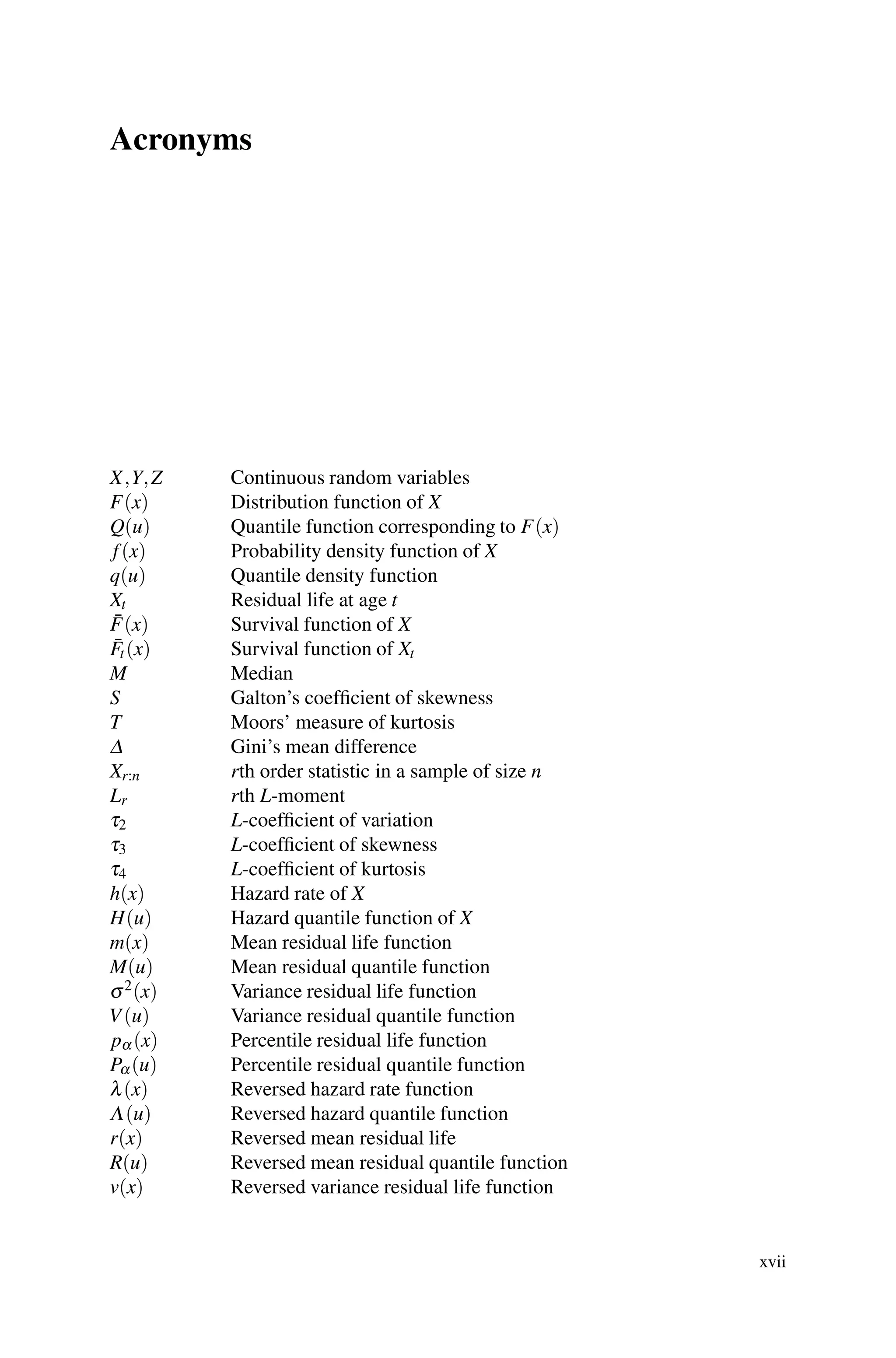
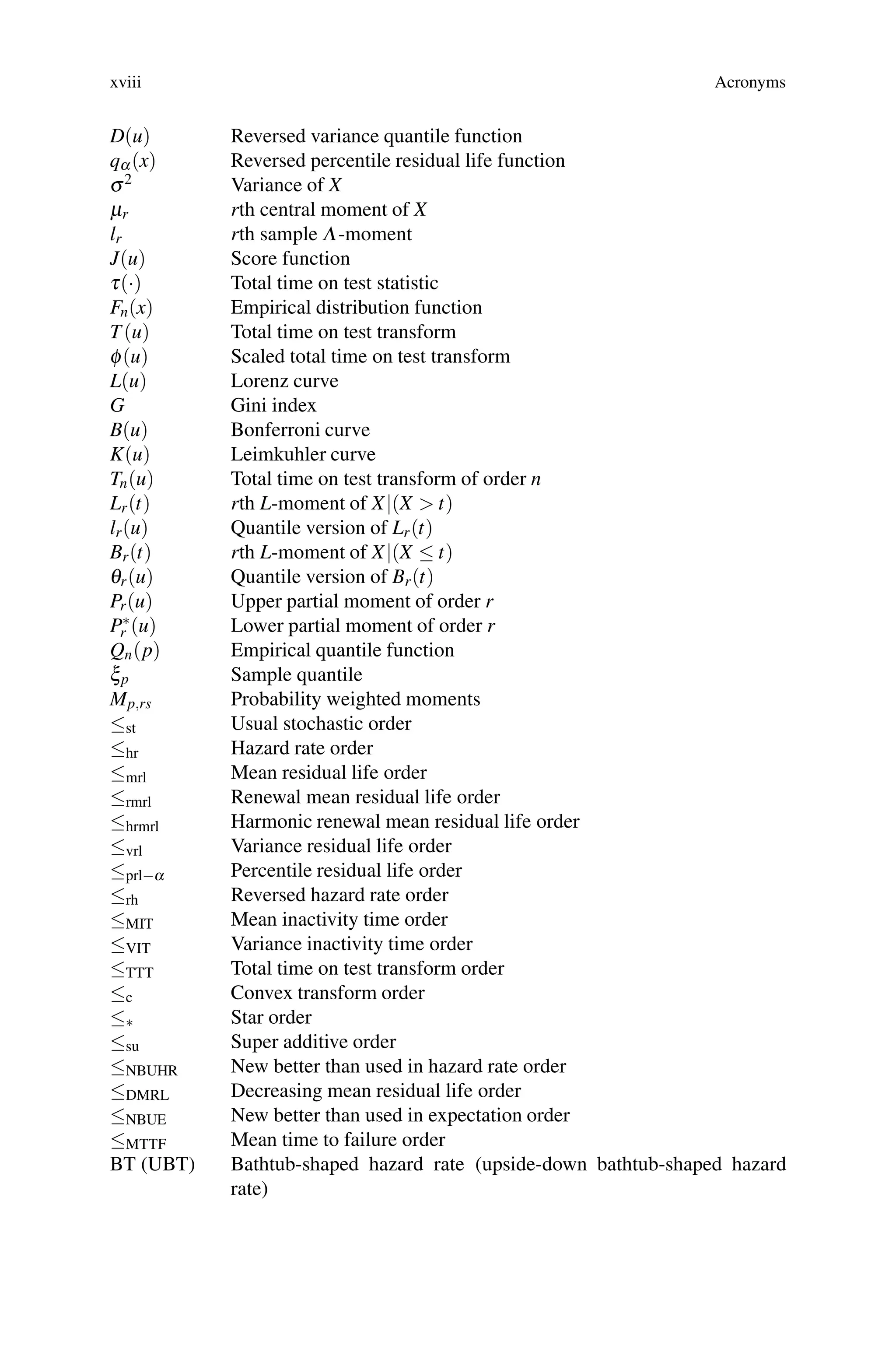


![2 1 Quantile Functions
an appropriate choice of the domain of observations, a better understanding of a
chance phenomenon can be achieved by the use of quantile functions, is fast gaining
acceptance.
Historically, many facts about the potential of quantiles in data analysis were
known even before the nineteenth century. It appears that the Belgian sociologist
Quetelet [499] initiated the use of quantiles in statistical analysis in the form of the
present day inter-quantile range. A formal representation of a distribution through
a quantile function was introduced by Galton (1822–1911) [206] who also initiated
the ordering of observations along with the concepts of median, quartiles and
interquartile range. Subsequently, the research on quantiles was directed towards
estimation problems with the aid of sample quantiles, their large sample behaviour
and limiting distributions (Galton [207, 208]). A major development in portraying
quantile functions to represent distributions is the work of Hastings et al. [264], who
introduced a family of distributions by a quantile function. This was refined later
by Tukey [568]. The symmetric distribution of Tukey [568] and his articulation
of exploratory data analysis sparked considerable interest in quantile functional
forms that continues till date. Various aspects of the Tukey family and general-
izations thereto were studied by a number of authors including Hogben [273],
Shapiro and Wilk [536], Filliben [197], Joiner and Rosenblatt [304], Ramberg
and Schmeiser [504], Ramberg [501], Ramberg et al. [502], MacGillivray [407],
Freimer et al. [203], Gilchrist [215] and Tarsitano [563]. We will discuss all these
models in Chap. 3. Another turning point in the development of quantile functions
is the seminal paper by Parzen [484], in which he emphasized the description
of a distribution in terms of the quantile function and its role in data modelling.
Parzen [485–487] exhibits a sequential development of the theory and application
of quantile functions in different areas and also as a tool in unification of various
approaches.
Quantile functions have several interesting properties that are not shared by
distributions, which makes it more convenient for analysis. For example, the sum
of two quantile functions is again a quantile function. There are explicit general dis-
tribution forms for the quantile function of order statistics. In Sect. 1.2, we mention
these and some other properties. Moreover, random numbers from any distribution
can be generated using appropriate quantile functions, a purpose for which lambda
distributions were originally conceived. The moments in different forms such as raw,
central, absolute and factorial have been used effectively in specifying the model,
describing the basic characteristics of distributions, and in inferential procedures.
Some of the methods of estimation like least squares, maximum likelihood and
method of moments often provide estimators and/or their standard errors in terms
of moments. Outliers have a significant effect on the estimates so derived. For
example, in the case of samples from the normal distribution, all the above methods
give sample mean as the estimate of the population mean, whose values change
significantly in the presence of an outlying observation. Asymptotic efficiency of the
sample moments is rather poor for heavy tailed distributions since the asymptotic
variances are mainly in terms of higher order moments that tend to be large in this
case. In reliability analysis, a single long-term survivor can have a marked effect](https://image.slidesharecdn.com/43349-250706133453-f9be5670/75/Quantile-Based-Reliability-Analysis-1st-Edition-N-Unnikrishnan-Nair-27-2048.jpg)
![4 1 Quantile Functions
Some important properties of quantile functions required in the sequel are as
follows.
1. From the definition of Q(u) for a general distribution function, we see that
(a) Q(u) is non-decreasing on (0,1) with Q(F(x)) ≤ x for all −∞ x ∞ for
which 0 F(x) 1;
(b) F(Q(u)) ≥ u for any 0 u 1;
(c) Q(u) is continuous from the left or Q(u−) = Q(u);
(d) Q(u+) = inf{x : F(x) u} so that Q(u) has limits from above;
(e) Any jumps of F(x) are flat points of Q(u) and flat points of F(x) are jumps
of Q(u).
2. If U is a uniform random variable over [0,1], then X = Q(U) has its distribution
function as F(x). This follows from the fact that
P(Q(U) ≤ x) = P(U ≤ F(x)) = F(x).
This property enables us to conceive a given data set as arising from the uniform
distribution transformed by the quantile function Q(u).
3. If T(x) is a non-decreasing function of x, then T(Q(u)) is a quantile function.
Gilchrist [215] refers to this as the Q-transformation rule. On the other hand, if
T(x) is non-increasing, then T(Q(1 − u)) is also a quantile function.
Example 1.1. Let X be a random variable with Pareto type II (also called Lomax)
distribution with
F(x) = 1 − αc
(x+ α)−c
, x 0; α,c 0.
Since F(x) is strictly increasing, setting F(x) = u and solving for x, we obtain
x = Q(u) = α[(1 − u)− 1
c − 1].
Taking T(X) = Xβ , β 0, we have a non-decreasing transformation which
results in
T(Q(u)) = αβ
[(1 − u)− 1
c − 1]β
.
When T(Q(u)) = y, we obtain, on solving for u,
u = G(y) = 1 −
⎛
⎝1 +
y
1
β
α
⎞
⎠
−c
which is a Burr type XII distribution with T(Q(u)) being the corresponding
quantile function.](https://image.slidesharecdn.com/43349-250706133453-f9be5670/75/Quantile-Based-Reliability-Analysis-1st-Edition-N-Unnikrishnan-Nair-29-2048.jpg)
![6 1 Quantile Functions
then
Q1(u) = λ−1
(−log(1 − u
1
θ ))
provides
G(x) = (1 − e−λx
)θ
,
the generalized or exponentiated exponential law (Gupta and Kundu [250]). In a
similar manner, Mudholkar and Srivastava [429] take the baseline distribution as
Weibull. For some recent results and survey of such models, we refer the readers
to Gupta and Gupta [240]. In Chap. 3, we will come across several quantile
functions that represent families of distributions containing some life distribu-
tions as special cases. They are highly flexible empirical models capable of
approximating many continuous distributions. The above transformation on these
models generates new proportional reversed hazards models of a general form.
The analysis of lifetime data employing such models seems to be an open issue.
Remark 1.1. From the form of G(x) above, it is clear that for positive integral
values of θ, it is simply the distribution function of the maximum of a random
sample of size θ from the exponential population with distribution function F(x)
above. Thus, G(x) may be simply regarded as the distribution function of the
maximum from a random sample of real size θ (instead of an integer). This
viewpoint was discussed by Stigler [547] under the general idea of ‘fractional
order statistics’; see also Rohatgi and Saleh [509].
Remark 1.2. Just as G(x) can be regarded as the distribution function of the
maximum from a random sample of (real) size θ from the population with
distribution function F(x), we can consider G∗(x) = 1 − (1 − F(x))θ as a
generalized form corresponding to the minimum of a random sample of (real)
size θ. The model G∗(x) is, of course, the familiar proportional hazards model.
It is important to mention here that these two models are precisely the ones
introduced by Lehmann [382], as early as in 1953, as stochastically ordered
alternatives for nonparametric tests of equality of distributions.
Remark 1.3. It is useful to bear in mind that for distributions closed under
minima such as exponential and Weibull (i.e., the distributions for which the
minima have the same form of the distribution but with different parameters),
the distribution function G(x) would provide a natural generalization while,
for distributions closed under maxima such as power and inverse Weibull (i.e.,
the distributions for which the maxima have the same form of the distribution
but with different parameters), the distribution function G∗(x) would provide a
natural generalization.
5. The sum of two quantile functions is again a quantile function. Likewise,
two quantile density functions, when added, produce another quantile density
function.](https://image.slidesharecdn.com/43349-250706133453-f9be5670/75/Quantile-Based-Reliability-Analysis-1st-Edition-N-Unnikrishnan-Nair-31-2048.jpg)


![1.4 Descriptive Quantile Measures 9
Example 1.4. Suppose the underlying distribution is logistic with distribution
function F(x) = 1/(1 + e−x) on the whole real line R. It is easily seen that
the corresponding quantile function is Q(u) = log
u
1−u . Further, suppose we
consider the distribution truncated on the left at 0, i.e., L = 0, for proposing a
lifetime model. Then, from the expression above and the fact that Q−1(0) = 1
2 ,
we arrive at the quantile function
QLT (u) = Q u + (1 − u)
1
2
= log
u + 1
2 (1 − u)
1 − u − 1
2 (1 − u)
= log
1 + u
1 − u
corresponding to the half-logistic distribution of Balakrishnan [47, 48]; see
Table 1.1.
1.3 Quantile Functions of Life Distributions
As mentioned earlier, we concentrate here on distributions of non-negative random
variables representing the lifetime of a component or unit. The distribution function
of such random variables is such that F(0−) = 0. Often, it is more convenient to
work with
F̄(x) = 1 − F(x) = P(X x),
which is the probability that the unit survives time (referred to as the age of the unit)
x. It is also called the reliability or survival function since it expresses the probability
that the unit is still reliable at age x.
In the previous section, some examples of quantile functions and a few methods
of obtaining them were explained. We now present in Table 1.1 quantile functions of
many distributions considered in the literature as lifetime models. The properties of
these distributions are discussed in the references cited below each of them. Models
like gamma, lognormal and inverse Gaussian do not find a place in the list as their
quantile functions are not in a tractable form. However, in the next chapter, we will
see quantile forms that provide good approximations to them.
1.4 Descriptive Quantile Measures
The advent of the Pearson family of distributions was a major turning point in
data modelling using distribution functions. The fact that members of the family
can be characterized by the first four moments gave an impetus to the extensive
use of moments in describing the properties of distributions and their fitting to
observed data. A familiar pattern of summary measures took the form of mean](https://image.slidesharecdn.com/43349-250706133453-f9be5670/75/Quantile-Based-Reliability-Analysis-1st-Edition-N-Unnikrishnan-Nair-34-2048.jpg)
![10 1 Quantile Functions
Table 1.1 Quantile functions of some lifetime distributions
No. Distribution F̄(x) Q(u)
1 Exponential exp[−λx] λ−1(−log(1−u))
(Marshall and Olkin [412]) x 0; λ 0
2 Weibull exp[−( x
σ )λ ] σ(−log(1−u))
1
λ
(Murthy et al. [434], x 0; λ,σ 0
Hahn and Shapiro [257])
3 Pareto II αc(x+α)−c α[(1−u))− 1
c −1]
(Marshall and Olkin [412]) x 0; α,c 0
4 Rescaled beta (1− x
R )c R[1−(1−u))
1
c ]
(Marshall and Olkin [412]) 0 ≤ x ≤ R; c,R 0
5 Half-logistic 2
1+exp
x
σ
−1
σ log
1+u
1−u
(Balakrishnan [47,48], x 0; σ 0
Balakrishnan and Wong [61])
6 Power 1−( x
α )β αu
1
β
(Marshall and Olkin [412]) 0 ≤ x ≤ α; α,β 0
7 Pareto I ( x
σ )−α σ(1−u)− 1
α
(Marshall and Olkin [412]) x σ 0; α,σ 0
8 Burr type XII (1+xc)−k [(1−u)
1
k −1]
1
c
(Zimmer et al. [604], x 0; c,k 0
Fry [204])
9 Gompertz exp[−B(Cx−1)
logC ] 1
logC [1− logClog(1−u)
B ]
(Lai and Xie [368]) x 0; B,C 0
10 Greenwich [225] (1+ x2
b2 )− a
2 b[(1−u)
2
a −1]
1
2
x ≥ 0; a,b 0
11 Kus [364] 1−eλe−βx
1−eλ − 1
β log[λ−1 log{1−(1−u)
x 0; λ,β 0 (1−e−λ )}]
12 Logistic exponential 1+(eλθ −1)k
1+(eλ(x+θ)−1)k
1
λ log[1+{(eλθ −1)k+u
1−u }
1
k ]
(Lan and Leemis [372]) x ≥ 0; λ 0,
k 0, θ ≥ 0
13 Dimitrakopoulou et al. [178] exp[1−(1+λxβ )α ] λ−1[{1−log(1−u)}
1
α −1]
1
β
x 0; α,β,λ 0
14 Log Weibull exp[−(log(1+ρx))k] ρ−1[exp(−log(1−u))
1
k −1]
(Avinadav and Raz [41]) x 0; ρ,k 0
15 Modified Weibull exp[−ασ(e( x
σ )λ
−1)] σ[log(1+ log(1−u)
ασ )]
1
λ
extension (Xie et al. [595]) x 0; α,σ,λ 0
16 Exponential power exp[e−(λt)α
−1] 1
λ [−log(1+log(1−u))]
1
α
(Paranjpe et al. [482]) x 0; λ,α 0
17 Generalized Pareto (1+ ax
b )− a+1
a b
a [(1−u)− a
a+1 −1]
(Lai and Xie [368]) x 0,b 0,a −1
18 Inverse Weibull 1−exp[−(σ
x )λ ] σ(−logu)− 1
λ
(Erto [188]) x 0; σ,λ 0
(continued)](https://image.slidesharecdn.com/43349-250706133453-f9be5670/75/Quantile-Based-Reliability-Analysis-1st-Edition-N-Unnikrishnan-Nair-35-2048.jpg)
![1.4 Descriptive Quantile Measures 11
Table 1.1 (continued)
No. Distribution F̄(x) Q(u)
19 Extended Weibull
θ exp[−( x
σ )λ ]
1−(1−θ)exp[−( x
σ )λ ]
σ[log θ+(1−θ)(1−u)
1−u ]
1
λ
(Marshall and Olkin [411]) x 0; θ,λ,σ 0
20 Generalized exponential 1−[1−exp(− x
σ )]θ σ[−log(1−u
1
θ )]
(Gupta et al. [239]) x 0; σ,θ 0
21 Exponentiated Weibull 1−[1−exp(− x
σ )λ ]θ σ[−log(1−u
1
θ )]
1
λ
(Mudholkar et al. [427]) x 0; σ,θ,λ 0
22 Generalized Weibull [1−λ( x
β )α ][ 1
λ
]
β[1−(1−u)λ
λ ]
1
α , λ = 0
(Mudholkar and Kollia [426]) x 0 for λ ≤ 0
0 x β
λ
1
α
, λ 0 β[−log(1−u)]
1
α , λ = 0
α,β 0
23 Exponential geometric (1− p)e−λx(1− pe−λx)−1 1
λ log(1−pu
1−u )
(Adamidis and
Loukas [18])
x 0, λ 0, 0 p 1
24 Log logistic (1+(αx)β )−1 α−1( u
1−u )
1
β
(Gupta et al. [237]) x 0, α,β 0
25 Generalized half-logistic 2(1−kx)1/k
1+(1−kx)1/k
1
k
1−
1−u
1+u
k
(Balakrishnan and
Sandhu [59],
0 ≤ x ≤ 1
k , k ≥ 0
Balakrishnan and
Aggarwala [49])
for location, variance for dispersion, and the Pearson’s coefficients β1 =
μ2
3
μ3
2
for
skewness and β2 = μ4
μ2
2
for kurtosis. While the mean and variance claimed universal
acceptance, several limitations of β1 and β2 were subsequently exposed. Some of
the concerns with regard to β1 are: (1) it becomes arbitrarily large or even infinite
making it difficult for comparison and interpretation as relatively small changes in
parameters produce abrupt changes, (2) it does not reflect the sign of the difference
(mean-median) which is a traditional basis for defining skewness, (3) there exist
asymmetric distributions with β1 = 0 and (4) instability of the sample estimate of
β1 while matching with the population value. Similarly, for a standardized variable
X, the relationship
E(X4
) = 1 +V(X2
) (1.5)
would mean that the interpretation of kurtosis depends on the concentration of the
probabilities near μ ± σ as well as in the tails of the distribution.
The specification of a distribution through its quantile function takes away the
need to describe a distribution through its moments. Alternative measures in terms
of quantiles that reduce the shortcomings of the moment-based ones can be thought
of. A measure of location is the median defined by](https://image.slidesharecdn.com/43349-250706133453-f9be5670/75/Quantile-Based-Reliability-Analysis-1st-Edition-N-Unnikrishnan-Nair-36-2048.jpg)
![12 1 Quantile Functions
M = Q(0.5). (1.6)
Dispersion is measured by the interquartile range
IQR = Q3 − Q1, (1.7)
where Q3 = Q(0.75) and Q1 = Q(0.25).
Skewness is measured by Galton’s coefficient
S =
Q1 + Q3 − 2M
Q3 − Q1
. (1.8)
Note that in the case of extreme positive skewness, Q1 → M while in the case of
extreme negative skewness Q3 → M so that S lies between −1 and +1. When the
distribution is symmetric, M = Q1+Q3
2 and hence S = 0. Due to the relation in (1.5),
kurtosis can be large when the probability mass is concentrated near the mean or in
the tails. For this reason, Moors [421] proposed the measure
T = [Q(0.875)− Q(0.625)+ Q(0.375)−Q(0.125)]/IQR (1.9)
as a measure of kurtosis. As an index, T is justified on the grounds that the
differences Q(0.875) − Q(0.625) and Q(0.375) − Q(0.125) become large (small)
if relatively small (large) probability mass is concentrated around Q3 and Q1
corresponding to large (small) dispersion in the vicinity of μ ± σ.
Given the form of Q(u), the calculations of all the coefficients are very simple,
as we need to only substitute the appropriate fractions for u. On the other hand,
calculation of moments given the distribution function involves integration, which
occasionally may not even yield closed-form expressions.
Example 1.5. Let X follow the Weibull distribution with (see Table 1.1)
Q(u) = σ(−log(1 − u))
1
λ .
Then, we have
M = Q
1
2
= σ(log2)
1
λ ,
S =
(log4)
1
λ + (log 4
3 )
1
λ − 2(log2)
1
λ
(log4)
1
λ −
log 4
3
1
λ
,
IQR = σ
(log4)
1
λ − log
4
3
1
λ
,](https://image.slidesharecdn.com/43349-250706133453-f9be5670/75/Quantile-Based-Reliability-Analysis-1st-Edition-N-Unnikrishnan-Nair-37-2048.jpg)
![1.4 Descriptive Quantile Measures 13
and
T =
(log8)
1
λ −
log 8
3
1
λ +
log 8
5
1
λ −
log 8
7
1
λ
(log4)
1
λ −
log 4
3
1
λ
.
The effect of a change of origin and scale on Q(u) and the above four measures
are of interest in later studies. Let X and Y be two random variables such that Y =
aX + b. Then,
FY (y) = P(Y ≤ y) = P X ≤
y− b
a
= FX
y− a
b
.
If QX (u) and QY (u) denote the quantile functions of X and Y, respectively,
FX
y− a
b
= u ⇒ QX (u) =
y− b
a
=
QY (u)− b
a
or
QY (u) = aQX (u)+ b.
So, we simply have
MY = QY (0.5) = aQX(0.5)+ b = aMX + b.
Similar calculations using (1.7), (1.8) and (1.9) yield
IQRY = aIQRX , SY = SX and TY = TX .
Other quantile-based measures have also been suggested for quantifying spread,
skewness and kurtosis. One measure of spread, similar to mean deviation in
the distribution function approach, is the median of absolute deviation from the
median, viz.,
A = Med(|X − M|). (1.10)
For further details and justifications for (1.10), we refer to Falk [194]. A second
popular measure that has received wide attention in economics is Gini’s mean
difference defined as
Δ =
∞
−∞
∞
−∞
|x− y|f(x)f(y)dxdy
= 2
∞
−∞
F(x)(1 − F(x))dx, (1.11)
where f(x) is the probability density function of X. Setting F(x) = u in (1.11), we
have](https://image.slidesharecdn.com/43349-250706133453-f9be5670/75/Quantile-Based-Reliability-Analysis-1st-Edition-N-Unnikrishnan-Nair-38-2048.jpg)
![14 1 Quantile Functions
Δ = 2
1
0
u(1 − u)q(u)du (1.12)
= 2
1
0
(2u − 1)Q(u)du. (1.13)
The expression in (1.13) follows from (1.12) by integration by parts. One
may use (1.12) or (1.13) depending on whether q(u) or Q(u) is specified.
Gini’s mean difference will be further discussed in the context of reliability in
Chap. 4.
Example 1.6. The generalized Pareto distribution with (see Table 1.1)
Q(u) =
b
a
(1 − u)− a
a+1 − 1
has its quantile density function as
q(u) =
b
a + 1
(1 − u)− a
a+1 −1
.
Then, from (1.12), we obtain
Δ =
2b
a + 1
1
0
u(1 − u)− a
a+1 du =
2b
a + 1
B 2,
1
a + 1
,
where B(m,n) =
1
0 tm−1(1−t)n−1dt is the complete beta function. Thus, we obtain
the simplified expression
Δ =
2b(a + 1)
a + 2
.
Hinkley [271] proposed a generalization of Galton’s measure of skewness of the
form
S(u) =
Q(u)+ Q(1 − u)− 2Q(0.5)
Q(u)− Q(1 − u)
. (1.14)
Obviously, (1.14) reduces to Galton’s measure when u = 0.75. Since (1.14)
is a function of u and u is arbitrary, an overall measure of skewness can be
provided as
S2 = sup
1
2 ≤u≤1
S(u).
Groeneveld and Meeden [227] suggested that the numerator and denominator
in (1.14) be integrated with respect to u to arrive at the measure](https://image.slidesharecdn.com/43349-250706133453-f9be5670/75/Quantile-Based-Reliability-Analysis-1st-Edition-N-Unnikrishnan-Nair-39-2048.jpg)
![1.4 Descriptive Quantile Measures 15
S3 =
1
1
2
{Q(u)+ Q(1 − u)− 2Q(0.5)}du
1
1
2
{Q(u)+ Q(1 − u)}du
.
Now, in terms of expectations, we have
1
1
2
Q(u)du =
x
M
xf(x)dx,
1
1
2
Q(1 − u)du =
1
2
0
Q(u)du =
M
0
xf(x)dx,
1
1
2
Q(0.5)du =
1
2
M,
and thus
S3 =
E(X)− M
∞
M xf(x)dx−
M
0 xf(x)dx
=
μ − M
E(|X − M|)
. (1.15)
The numerator of (1.15) is the traditional term (being the difference between the
mean and the median) indicating skewness and the denominator is a measure of
spread used for standardizing S3. Hence, (1.15) can be thought of as an index of
skewness in the usual sense. If we replace the denominator by the standard deviation
σ of X, the classical measure of skewness will result.
Example 1.7. Consider the half-logistic distribution with (see Table 1.1)
Q(u) = σ log
1 + u
1 − u
,
μ =
1
0
Q(u)du = σ log4,
1
1
2
Q(u)du = σ log16 −
3
2
log3 ,
1
2
0
Q(u)du = σ
3
2
log3 − 2log2 ,
and hence S3 = log(4
3 )/log(64
27 ).
Instead of using quantiles, one can also use percentiles to define skewness.
Galton [206] in fact used the middle 50 % of observations, while Kelly’s measure
takes 90 % of observations to propose the measure
S4 =
Q(0.90)+ Q(0.10)− 2M
Q(0.90)− Q(0.10)
.](https://image.slidesharecdn.com/43349-250706133453-f9be5670/75/Quantile-Based-Reliability-Analysis-1st-Edition-N-Unnikrishnan-Nair-40-2048.jpg)
![16 1 Quantile Functions
For further discussion of alternative measures of skewness and kurtosis, a review of
the literature and comparative studies, we refer to Balanda and MacGillivray [63],
Tajuddin [559], Joannes and Gill [299], Suleswki [552] and Kotz and Seier [355].
1.5 Order Statistics
In life testing experiments, a number of units, say n, are placed on test and the
quantity of interest is their failure times which are assumed to follow a distribution
F(x). The failure times X1,X2,...,Xn of the n units constitute a random sample
of size n from the population with distribution function F(x), if X1,X2,...,Xn are
independent and identically distributed as F(x). Suppose the realization of Xi in
an experiment is denoted by xi. Then, the order statistics of the random sample
(X1,X2,...,Xn) are the sample values placed in ascending order of magnitude de-
noted by X1:n ≤ X2:n ≤ ··· ≤ Xn:n, so that X1:n = min1≤i≤n Xi and Xn:n = max1≤i≤n Xi.
The sample median, denoted by m, is the value for which approximately 50 % of the
observations are less than m and 50 % are more than m. Thus
m =
⎧
⎨
⎩
Xn+1
2 :n if n is odd
1
2 (Xn
2 :n + Xn
2 +1:n) if n is even.
(1.16)
Generalizing, we have the percentiles. The 100p-th percentile, denoted by xp, in
the sample corresponds to the value for which approximately np observations are
smaller than this value and n(1 − p) observations are larger. In terms of order
statistics we have
xp =
X[np]:n if 1
2n p 0.5
X(n+1)−[n(1−p)] if 0.5 p 1 − 1
2n
, (1.17)
where the symbol [t] is defined as [t] = r whenever r − 0.5 ≤ t r + 0.5, for all
positive integers r. We note that in the above definition, if xp is the ith smallest
observation, then the ith largest observation is x1−p. Obviously, the median m is the
50th percentile and the lower quartile q1 and the upper quartile q3 of the sample are,
respectively, the 25th and 75th percentiles. The sample interquartile range is
iqr = q3 − q1. (1.18)
All the sample descriptive measures are defined in terms of the sample median,
quartiles and percentiles analogous to the population measures introduced in
Sect. 1.4. Thus, iqr in (1.18) describes the spread, while
s =
q3 + q1 − 2m
q3 − q1
(1.19)](https://image.slidesharecdn.com/43349-250706133453-f9be5670/75/Quantile-Based-Reliability-Analysis-1st-Edition-N-Unnikrishnan-Nair-41-2048.jpg)
![1.5 Order Statistics 17
and
t =
e7 − e5 + e3 − e1
iqr
, (1.20)
where ei = i
8 , i = 1,3,5,7, describes the skewness and kurtosis.
Parzen [484] introduced the empirical quantile function
Q̄(u) = F−1
n (u) = inf(x : Fn(x) ≥ u),
where Fn(x) is the proportion of X1,X2,...,Xn that is at most x. In other words,
Q̄(u) = Xr:n for
r − 1
n
u
r
n
, r = 1,2,...,n, (1.21)
which is a step function with jump 1
n . For u = 0, Q̄(u) is taken as X1:n or a
natural minimum if one is available. In the case of lifetime variables, this becomes
Q̄(0). When a smooth function is required for Q̄(u), Parzen [484] suggested the
use of
Q̄1(u) = n
r
n
− u
Xr−1:n + n u −
r − 1
n
Xr:n
for r−1
n ≤ u ≤ r
n , r = 1,2,...,n. The corresponding empirical quantile density
function is
q̄1(u) =
d
du
Q̄1(u) = n(Xr:n − Xr−1:n), for
r − 1
n
u
r
n
.
In this set-up, we have qi = Q̄( i
4 ), i = 1,3 and ei = Q̄( i
8 ), i = 1,3,7,8.
It is well known that the distribution of the rth order statistic Xr:n is given by
Arnold et al. [37]
Fr(x) = P(Xr:n ≤ x) =
n
∑
k=r
n
k
Fk
(x)(1 − F(x))n−k
. (1.22)
In particular, Xn:n and X1:n have their distributions as
Fn(x) = Fn
(x) (1.23)
and
F1(x) = 1 − (1 − F(x))n
. (1.24)](https://image.slidesharecdn.com/43349-250706133453-f9be5670/75/Quantile-Based-Reliability-Analysis-1st-Edition-N-Unnikrishnan-Nair-42-2048.jpg)
![18 1 Quantile Functions
Recalling the definitions of the beta function
B(m,n) =
1
0
tm−1
(1 −t)n−1
dt, m,n 0,
and the incomplete beta function ratio
Ix(m,n) =
Bx(m,n)
B(m,n)
,
where
Bx(m,n) =
x
0
tm−1
(1 −t)n−1
dt,
we have the upper tail of the binomial distribution and the incomplete beta function
ratio to be related as (Abramowitz and Stegun [15])
n
∑
k=r
n
k
pk
(1 − p)n−k
= Ip(r,n − r + 1). (1.25)
Comparing (1.22) and (1.25) we see that, if a sample of n observations from a
distribution with quantile function Q(u) is ordered, then the quantile function of
the rth order statistic is given by
Qr(ur) = Q(I−1
ur
(r,n − r + 1)), (1.26)
where
ur = Iu(r,n − r + 1) (1.27)
and I−1
is the inverse of the beta function ratio I. Thus, the quantile function of
the rth order statistic has an explicit distributional form, unlike the expression for
distribution function in (1.22). However, the expression for Qr(ur) is not explicit
in terms of Q(u). This is not a serious handicap as the Iu(·,·) function is tabulated
for various values of n and r (Pearson [489]) and also available in all statistical
softwares for easy computation. The distributions of Xn:n and X1:n have simple
quantile forms
Qn(un) = Q u
1
n
n
and
Q1(u1) = Q[1 − (1 − u1)
1
n ].](https://image.slidesharecdn.com/43349-250706133453-f9be5670/75/Quantile-Based-Reliability-Analysis-1st-Edition-N-Unnikrishnan-Nair-43-2048.jpg)
![1.5 Order Statistics 19
The probability density function of Xr:n becomes
fr(x) =
n!
(r − 1)!(n − r)!
Fr−1
(x)(1 − F(x))n−r
f(x)
and so
μr:n = E(Xr:n) =
xfr(x)dx
=
n!
(r − 1)!(n − 1)!
1
0
ur−1
(1 − u)n−r
Q(u)du. (1.28)
This mean value is referred to as the rth mean rankit of X. For reasons explained
earlier with reference to the use of moments, often the median rankit
Mr:n = Q(I−1
0.5 (r,n − r + 1)), (1.29)
which is robust, is preferred over the mean rankit.
The importance and role of order statistics in the study of quantile function
become clear from the discussions in this section. Added to this, there are several
topics in reliability analysis in which order statistics appear quite naturally. One of
them is system reliability. We consider a system consisting of n components whose
lifetimes X1,X2,...,Xn are independent and identically distributed. The system is
said to have a series structure if it functions only when all the components are func-
tioning, and the lifetime of this system is the smallest among the Xi’s or X1:n. In the
parallel structure, on the other hand, the system functions if and only if at least one
of the components work, so that the system life is Xn:n. These two structures are em-
bedded in what is called a k-out-of-n system, which functions if and only if at least
k of the components function. The lifetime of such a system is obviously Xn−k+1:n.
In life testing experiments, when n identical units are put on test to ascertain
their lengths of life, there are schemes of sampling wherein the experimenter need
not have to wait until all units fail. The experimenter may choose to observe only
a prefixed number of failures of, say, n − r units and terminate the experiment
as soon as the (n − r)th unit fails. Thus, the lifetimes of r units that are still
working get censored. This sampling scheme is known as type II censoring. The
data consists of realizations of X1:n,X2:n,...,Xn−r:n. Another sampling scheme is
to prefix a time T∗ and observe only those failures that occur up to time T∗. This
scheme is known as type I censoring, and in this case the number of failures to
be observed is random. One may refer to Balakrishnan and Cohen [51] and Cohen
[154] for various methods of inference for type I and type II censored samples from
a wide array of lifetime distributions. Yet another sampling scheme is to prefix the
number of failures at n − r and also a time T∗. If (n − r) failures occur before time
T∗, then the experiment is terminated; otherwise, observe all failures until time
T∗. Thus, the time of truncation of the experiment is now min(T,Xn−r:n). This is
referred to as type I hybrid censoring; see Balakrishnan and Kundu [53] for an
overview of various developments on this and many other forms of hybrid censoring](https://image.slidesharecdn.com/43349-250706133453-f9be5670/75/Quantile-Based-Reliability-Analysis-1st-Edition-N-Unnikrishnan-Nair-44-2048.jpg)
![20 1 Quantile Functions
schemes. A third important application of order statistics is in the construction of
tests regrading the nature of ageing of a device; see Lai and Xie [368]. For an
encyclopedic treatment on the theory, methods and applications of order satistics,
one may refer to Balakrishnan and Rao [56,57].
1.6 Moments
The emphasis given to quantiles in describing the basic properties of a distribution
does not in any way minimize the importance of moments in model specification and
inferential problems. In this section, we look at various types of moments through
quantile functions. The conventional moments
μ
r = E(Xr
) =
∞
0
xr
f(x)dx
are readily expressible in terms of quantile functions, by the substitution x =
Q(u), as
μ
r =
1
0
{Q(u)}r
du. (1.30)
In particular, as already seen, the mean is
μ =
1
0
Q(u)du =
1
0
(1 − u)q(u)du. (1.31)
The central moments and other quantities based on it are obtained through the well-
known relationships they have with the raw moments μ
r in (1.30).
Some of the difficulties experienced while employing the moments in descriptive
measures as well as in inferential problems have been mentioned in the previous
sections. The L-moments to be considered next can provide a competing alternative
to the conventional moments. Firstly, by definition, they are expected values of
linear functions of order statistics. They have generally lower sampling variances
and are also robust against outliers. Like the conventional moments, L-moments can
be used as summary measures (statistics) of probability distributions (samples), to
identify distributions and to fit models to data. The origin of L-moments can be
traced back to the work on linear combination of order statistics in Sillito [537] and
Greenwood et al. [226]. It was Hosking [276] who presented a unified theory on
L-moments and made a systematic study of their properties and role in statistical
analysis. See also Hosking [277, 279, 280] and Hosking and Wallis [282] for more
elaborate details on this topic.
The rth L-moment is defined as
Lr =
1
r
r−1
∑
k=0
(−1)k r − 1
k
E(Xr−k:r), r = 1,2,3,... (1.32)](https://image.slidesharecdn.com/43349-250706133453-f9be5670/75/Quantile-Based-Reliability-Analysis-1st-Edition-N-Unnikrishnan-Nair-45-2048.jpg)
![1.6 Moments 21
Using (1.28), we can write
Lr =
1
r
r−1
∑
k=0
(−1)k r − 1
k
r!
(r − k − 1)!k!
1
0
ur−k−1
(1 − u)k
Q(u)du.
Expanding (1 − u)k in powers of u using binomial theorem and combining powers
of u, we get
Lr =
1
0
r−1
∑
k=0
(−1)r−1−k r − 1
k
r − 1 + k
k
uk
Q(u)du. (1.33)
Jones [306] has given an alternative method of establishing the last relationship. In
particular, we obtain:
L1 =
1
0
Q(u)du = μ, (1.34)
L2 =
1
0
(2u − 1)Q(u)du, (1.35)
L3 =
1
0
(6u2
− 6u + 1)Q(u)du, (1.36)
L4 =
1
0
(20u3
− 30u2
+ 12u − 1)Q(u)du. (1.37)
Sometimes, it is convenient (to avoid integration by parts while computing the
integrals in (1.34)–(1.37)) to work with the equivalent formulas
L1 =
1
0
(1 − u)q(u)du, (1.38)
L2 =
1
0
(u − u2
)q(u)du, (1.39)
L3 =
1
0
(3u2
− 2u3
− u)q(u)du, (1.40)
L4 =
1
0
(u − 6u2
+ 10u3
− 5u4
)q(u)du. (1.41)
Example 1.8. For the exponential distribution with parameter λ, we have
Q(u) = −λ−1
log(1 − u) and q(u) =
1
λ(1 − u)
.](https://image.slidesharecdn.com/43349-250706133453-f9be5670/75/Quantile-Based-Reliability-Analysis-1st-Edition-N-Unnikrishnan-Nair-46-2048.jpg)
![22 1 Quantile Functions
Hence, using (1.38)–(1.41), we obtain
L1 =
1
0
1
λ
du = λ−1
,
L2 =
1
0
u(1 − u)q(u)du =
1
0
u
λ
du = (2λ)−1
,
L3 =
1
0
u(1 − u)(2u − 1)q(u)du = (6λ)−1
,
L4 =
1
0
u(1 − u)(1 − 5u + 5u2
)q(u)du = (12λ)−1
.
More examples are presented in Chap. 3 when properties of various distributions are
studied.
The L-moments have the following properties that distinguish themselves from
the usual moments:
1. The L-moments exist whenever E(X) is finite, while additional restrictions may
be required for the conventional moments to be finite for many distributions;
2. A distribution whose mean exists is characterized by (Lr : r = 1,2,...). This
result can be compared with the moment problem discussed in probability theory.
However, any set that contains all L-moments except one is not sufficient to
characterize a distribution. For details, see Hosking [279,280];
3. From (1.12), we see that L2 = 1
2 Δ, and so L2 is a measure of spread. Thus,
the first (being the mean) and second L-moments provide measures of location
and spread. In a recent comparative study of the relative merits of the variance
and the mean difference Δ, Yitzhaki [596] noted that the mean difference is
more informative than the variance in deriving properties of distributions that
depart from normality. He also compared the algebraic structure of variance
and Δ and examined the relative superiority of the latter from the stochastic
dominance, exchangability and stratification viewpoints. For further comments
on these aspects and some others in the reliability context, see Chap. 7;
4. Forming the ratios τr = Lr
L2
, r = 3,4,..., for any non-degenerateX with μ ∞, the
result |τr| 1 holds. Hence, the quantities τr’s are dimensionless and bounded;
5. The skewness and kurtosis of a distribution can be ascertained through the
moment ratios. The L-coefficient of skewness is
τ3 =
L3
L2
(1.42)
and the L-coefficient of kurtosis is
τ4 =
L4
L2
. (1.43)
These two measures satisfy the criteria presented for coefficients of skewness
and kurtosis in terms of order relations. The range of τ3 is (−1,1) while that
of τ4 is 1
4 (5τ2
3 − 1) ≤ τ4 1. These results are proved in Hosking [279] and](https://image.slidesharecdn.com/43349-250706133453-f9be5670/75/Quantile-Based-Reliability-Analysis-1st-Edition-N-Unnikrishnan-Nair-47-2048.jpg)
![1.6 Moments 23
Jones [306] using different approaches. It may be observed that both τ3 and τ4
are bounded and do not assume arbitrarily large values as β1 (for example, in the
case of F(x) = 1 − x−3, x 1);
6. The ratio
τ2 =
L2
L1
(1.44)
is called L-coefficient of variation. Since X is non-negative in our case, L1 0,
L2 0 and further
L2 =
1
0
u(1 − u)q(u)du
1
0
(1 − u)q(u)du = L1
so that 0 τ2 1.
The above properties of L-moments have made them popular in diverse applications,
especially in hydrology, civil engineering and meteorology. Several empirical
studies (as the one by Sankarasubramonian and Sreenivasan [517]) comparing L-
moments and the usual moments reveal that estimates based on the former are less
sensitive to outliers. Just as matching the population and sample moments for the
estimation of parameters, the same method (method of L-moments) can be applied
with L-moments as well. Asymptotic approximations to sampling distributions are
better achieved with L-moments. An added advantage is that standard errors of
sample L-moments exist whenever the underlying distribution has a finite variance,
whereas for the usual moments this may not be enough in many cases.
When dealing with the conventional moments, the (β1,β2) plot is used as a
preliminary tool to discriminate between candidate distributions for the data. For
example, if one wishes to choose a distribution from the Pearson family as a model,
(β1,β2) provide exclusive classification of the members of this family. Distributions
with no shape parameters are represented by points in the β1-β2 plane, those with a
single shape parameter have their (β1,β2) values lie on the line 2β2 − 3β1 − 6 = 0,
while two shape parameters in the distribution ensure that for them, (β1,β2) falls in
a region between the lines 2β2 − 3β1 − 6 = 0 and β2 − β1 − 1 = 0. These cases are,
respectively, illustrated by the exponential distribution (which has (β1,β2) = (4,9)
as a point), the gamma family and the beta family; see Johnson et al. [302]
for details. In a similar manner, one can construct (τ2,τ3)-plots or (τ3,τ4)-plots
for distribution functions or quantile functions to give a visual identification of
which distribution can be expected to fit a given set of observations. Vogel and
Fennessey [574] articulate the need for such diagrams and provide several examples
on how to construct them. Some refinements of the L-moments are also studied in
the name of trimmed L-moments (Elamir and Seheult [187], Hosking [281]) and
LQ-moments (Mudholkar and Hutson [424]).
Example 1.9. The L-moments of the exponential distribution were calculated ear-
lier in Example 1.8. Applying the formulas for τ2, τ3 and τ4 in (1.44), (1.42)
and (1.43), we have](https://image.slidesharecdn.com/43349-250706133453-f9be5670/75/Quantile-Based-Reliability-Analysis-1st-Edition-N-Unnikrishnan-Nair-48-2048.jpg)
![24 1 Quantile Functions
τ2 =
1
2
, τ3 =
1
3
, τ4 =
1
6
.
Thus, (τ2,τ3) = (1
2 , 1
3 ) and (τ3,τ4) = (1
3 , 1
6 ) are points in the τ2-τ3 and τ3-τ4 planes,
respectively.
Example 1.10. The random variable X has generalized Pareto distribution with
Q(u) =
b
a
{(1 − u)− a
a+1 − 1}, a −1, b 0.
Then, straightforward calculations yield
L1 = b, L2 = b(a + 1)(a + 2)−1
,
L3 = b(a + 1)(2a + 1)[(2a +3)(a +2)]−1
,
L4 = b(a + 1)(6a2
+ 7a + 2)[(a + 2)(2a+3)(3a+4)]−1
,
so that
τ2 =
a + 1
a + 2
, τ3 =
2a + 1
2a + 3
and τ4 =
6a2 + 7a + 2
6a2 + 17a + 12
.
Then, eliminating a between τ2 and τ3, we obtain
τ3 =
3τ2 − 1
τ2 + 1
.
Thus, the plot of (τ2,τ3) for all values of a and b lies on the curve
(τ2 + 1)(3 − τ3) = 4. Note that the exponential plot is (1
2 , 1
3 ) which lies on the curve
when a → 0. The estimation and other related inferential problems are discussed
in Chap. 7.
We now present probability weighted moments (PWM) which is a forerunner
to the concept of L-moments. Introduced by Greenwood et al. [226], PWMs are of
considerable interest when the distribution is expressed in quantile form. The PWMs
are defined as
Mp,r,s = E[X p
Fr
(X)F̄s
(X)], (1.45)
where p,r,s are non-negative real numbers and E|X|p
∞. Two special cases
of (1.45) in general use are
βp,r = E(X p
Fr
(X))
=
xp
Fr
(x)f(x)dx
=
1
0
(Q(u))p
ur
du (1.46)](https://image.slidesharecdn.com/43349-250706133453-f9be5670/75/Quantile-Based-Reliability-Analysis-1st-Edition-N-Unnikrishnan-Nair-49-2048.jpg)