Matrixexponential Distributions In Applied Probability 1st Edition Mogens Bladt
Matrixexponential Distributions In Applied Probability 1st Edition Mogens Bladt
Matrixexponential Distributions In Applied Probability 1st Edition Mogens Bladt
Matrixexponential Distributions In Applied Probability 1st Edition Mogens Bladt
Matrixexponential Distributions In Applied Probability 1st Edition Mogens Bladt
1.
Matrixexponential Distributions InApplied
Probability 1st Edition Mogens Bladt download
https://ebookbell.com/product/matrixexponential-distributions-in-
applied-probability-1st-edition-mogens-bladt-5881062
Explore and download more ebooks at ebookbell.com
2.
Here are somerecommended products that we believe you will be
interested in. You can click the link to download.
Type Typography Highlights From Matrix The Review For Printers And
Bibliophiles Matrix
https://ebookbell.com/product/type-typography-highlights-from-matrix-
the-review-for-printers-and-bibliophiles-matrix-11052164
Matrix And Tensor Decompositions In Signal Processing Volume 2 Grard
Favier
https://ebookbell.com/product/matrix-and-tensor-decompositions-in-
signal-processing-volume-2-grard-favier-46575482
Matrix And Finite Element Analyses Of Structures Madhujit Mukhopadhyay
https://ebookbell.com/product/matrix-and-finite-element-analyses-of-
structures-madhujit-mukhopadhyay-47508134
Matrix Algebra James E Gentle
https://ebookbell.com/product/matrix-algebra-james-e-gentle-47913378
3.
Matrix Lauren Groff
https://ebookbell.com/product/matrix-lauren-groff-48269978
MatrixPathobiology And Angiogenesis Evangelia Papadimitriou
https://ebookbell.com/product/matrix-pathobiology-and-angiogenesis-
evangelia-papadimitriou-48737274
Matrix Mathematics Theory Facts And Formulas With Application To
Linear Systems Theory 1st Edition Dennis S Bernstein
https://ebookbell.com/product/matrix-mathematics-theory-facts-and-
formulas-with-application-to-linear-systems-theory-1st-edition-dennis-
s-bernstein-50142526
Matrix Discrete Element Analysis Of Geological And Geotechnical
Engineering 1st Edition Chun Liu
https://ebookbell.com/product/matrix-discrete-element-analysis-of-
geological-and-geotechnical-engineering-1st-edition-chun-liu-50558784
Matrix Head And Neck Reconstruction Scalable Reconstructive Approaches
Organized By Defect Location 1st Edition Brendan C Stack Jr Editor
https://ebookbell.com/product/matrix-head-and-neck-reconstruction-
scalable-reconstructive-approaches-organized-by-defect-location-1st-
edition-brendan-c-stack-jr-editor-51055756
5.
ProbabilityTheory and StochasticModelling 81
Mogens Bladt
Bo Friis Nielsen
Matrix-Exponential
Distributions in
Applied Probability
6.
Probability Theory andStochastic Modelling
Volume 81
Editors-in-chief
Søren Asmussen, Aarhus, Denmark
Peter W. Glynn, Stanford, CA, USA
Yves Le Jan, Orsay, France
Advisory Board
Martin Hairer, Coventry, UK
Peter Jagers, Gothenburg, Sweden
Ioannis Karatzas, New York, NY, USA
Frank P. Kelly, Cambridge, UK
Andreas E. Kyprianou, Bath, UK
Bernt Øksendal, Oslo, Norway
George Papanicolaou, Stanford, CA, USA
Etienne Pardoux, Marseille, France
Edwin Perkins, Vancouver, BC, Canada
Halil Mete Soner, Zürich, Switzerland
7.
The Probability Theoryand Stochastic Modelling series is a merger and
continuation of Springer’s two well established series Stochastic Modelling and
Applied Probability and Probability and Its Applications series. It publishes
research monographs that make a significant contribution to probability theory or
an applications domain in which advanced probability methods are fundamental.
Books in this series are expected to follow rigorous mathematical standards, while
also displaying the expository quality necessary to make them useful and accessible
to advanced students as well as researchers. The series covers all aspects of modern
probability theory including
• Gaussian processes
• Markov processes
• Random fields, point processes and random sets
• Random matrices
• Statistical mechanics and random media
• Stochastic analysis
as well as applications that include (but are not restricted to):
• Branching processes and other models of population growth
• Communications and processing networks
• Computational methods in probability and stochastic processes, including
simulation
• Genetics and other stochastic models in biology and the life sciences
• Information theory, signal processing, and image synthesis
• Mathematical economics and finance
• Statistical methods (e.g. empirical processes, MCMC)
• Statistics for stochastic processes
• Stochastic control
• Stochastic models in operations research and stochastic optimization
• Stochastic models in the physical sciences
More information about this series at http://www.springer.com/series/13205
8.
Mogens Bladt •Bo Friis Nielsen
Matrix-Exponential
Distributions in
123
Applied Probability
Preface
In 1844, RobertLeslie Ellis published a paper on calculating the total lifetime of n
independent individuals, each of them having an exponentially distributed lifetime.
One of the potential applications of Ellis’s research, as he states, was as follows:
The method of this paper extends m.m. to the case in which we seek to determine the degree
of improbability that the average length of the reigns of a series of kings shall exceed by a
given quantity the average deduced from authentic history.
Later, when A.K. Erlang at the beginning of the twentieth century suggested the
use of what is known today as the Erlang distributions, the aim was to provide an
adequate model for the duration of telephone calls as registered at the Copenhagen
Telephone Company. Instead of using an exponential distribution directly as a model
for “lifetimes” (e.g., duration of telephone calls), the idea was to decompose the
lifetimes into fictitious bits, each of which could be assumed to have an exponential
distribution. While the stages Ellis had in mind were observable lifetimes (perhaps
of kings), Erlang’s idea was to introduce fictitious stages in order to improve the
overall fit of a theoretical model to real data. In 1953, A. Jensen took a further step
in formulating the method of stages in terms of Markov jump processes.
In 1955, D.R. Cox wrote an article on the use of complex probabilities in the the-
ory of stochastic processes based on the use of rational Laplace transforms, which
may be considered a forerunner of what would later become known as matrix-
exponential distributions. Cox did not make use of matrix notation, which was
not omnipresent in those days, but performed formal manipulations with “complex
probabilities.” The matrix-exponential methodology may be seen as the ultimate
generalization of the methods of stages (both Erlang’s and Jensen’s).
In the 1970s, several publications by M.F. Neuts and coauthors laid the ground
for the development of the field of matrix-analytic methods in applied probability.
They formulated their expressions in terms of matrices, and the method gained mo-
mentum, proving able to solve complex problems in stochastic modeling explicitly
in terms of matrix equations or functions of matrices, usually restricted to matrix ex-
ponentials. It became folklore in the area that if you could prove something for the
exponential distribution, then you would be able to extend it to phase-type (and later
v
11.
vi Preface
even tomatrix-exponential) distributions as well. As we will see in this book, many
formulas that hold when some underlying distributions are assumed exponential are
valid also for matrix-exponential distributions almost by simply replacing the scalar
intensities with matrices. We take this a step further and use functional calculus in
several places to formulate results in terms of functions of matrices (more general
than the exponential).
The aim of this textbook, written at the graduate level, is to present a unified the-
ory of phase-type and matrix-exponential methods. As we will demonstrate through-
out the book, the two techniques supplement each other. We are concerned with their
distributional properties, applications, and estimation. When dealing with phase-
type distributions, we will usually employ a probabilistic approach, which will turn
out to provide a powerful technique for obtaining even complex formulas in a rather
simple way. The probabilistic way of reasoning is a fully rigorous method based
on sample path arguments, which may leave the student perplexed at first. But
don’t despair, it is an “acquired taste,” one that usually becomes greatly appreci-
ated. Matrix-exponential distributions, on the other hand, lack the natural potential
for probabilistic reasoning, and most results are proved using analytic means or by
an imitated probabilistic method based on flows.
In terms of applications, we have decided to present general tools that can be
applied to a variety of stochastic models. It is our hope that in this way, applications
different from those already provided in the text will be easier to accommodate. Fi-
nally, we provide a couple of chapters on the estimation of phase-type distributions
and Markov jump processes. We believe that these are interesting topics on their
own and important for “real” applications whenever a stochastic model needs to be
calibrated to empirical evidence.
The book contains both original results and material that is presented in a text-
book for the first time. The section on order statistics for phase-type distributions has
not previously been presented in a book, while the corresponding results on order
statistics for matrix-exponential distributions are new. In the treatment of time aver-
ages and their asymptotics, the methods employed from functional calculus (func-
tions of matrices) have allowed us to present new and more general results. In the
applications of risk processes that depend on their current reserve, we have taken a
more elaborate approach than the original paper for the sake of mathematical trans-
parency. For other parts, derivations may be different from the original sources. This
is in particular true for parts using functional calculus where we are able to substan-
tially shorten proofs and gain generality, and in other parts using some results from
integrals of matrix exponentials that enable us to provide explicit solutions to results
that were previously known as solutions to certain differential equations, or equiv-
alently, to certain unsolved integrals. This is, for example, the case in the sections
on occupation times in Markov jump processes and on the estimation of phase-type
distributions using the EM algorithm.
We have intended to present a textbook that may be used for lecture courses.
12.
Preface vii
Basic knowledge:
1.1,1.2, 1.3
3.1
Full course
2.1–2.4
3.2–3.5
4.1–4.6
5.1–5.7
6.1–6.3 7.1–
7.3,7.4∗
9.1–9-6
11.3–
11.4
Applications
course
5.1,
5.3–5.5 8.1
12.1–
12.8
13.1–
13.8
The ME
course
3.2–3.5
4.1–4.6,
4.7∗
5.1–5.7
6.1–6.3
11.1, 11.2
The short
course
5.1, 5.3
6.1,
6.2.1,
6.2.3
In the diagram we suggest four different courses. The basic knowledge part
is common for all courses. The short course refers to a 7.5 ECTS (European
Credit Transfer and Accumulation System) course covering the basic theory and
applications of phase-type distributions. The full course, depending on the prepara-
tion of the students, can be carried out in two to three blocks of 7.5 ECTS. This is a
comprehensive course covering most theory and applications of matrix-exponential
distributions. The ME course is a specialized course focusing on matrix-exponential
distributions (1 to 2 times 7.5 ECTS), while the last course on applications is di-
rected to professionals and researchers aiming at modeling and applying phase-type
methods. This course could be given within 1 to 2 units of 7.5 ECTS.
We owe our thanks to Martin Bladt and Emil Friis Frølich who did a wonderful
job by checking the mathematics of the entire book, and we appreciate the com-
ments of Azucena Campillo and Oscar Peralta on earlier drafts of the manuscript.
At Springer special thanks go to Donna Chernyk for her professional guidance and
to David Kramer, who did an impressive job in the final editing stage.
13.
viii Preface
We aregrateful to Søren Asmussen for his continuing interest and valuable com-
ments throughout the whole process. Last, but not least, we express our gratitude to
our families for their patience and understanding during the long process, usually
referred to simply as “the book”!
Copenhagen and Mexico City, Mogens Bladt
April, 2017 Bo Friis Nielsen
Notation
1{x∈A},1A(x),1{x ∈ A}: indicator function for A
δx(y) : Kronecker delta, function that is one if x = y and
zero otherwise
δi, j,δi j,δi− j : number that is one if i = j, zero otherwise
X,Y,... : random variables are usually uppercase nonbold
roman letters
Xi:n : the ith order statistic out of n
{Xt}t∈I,{X(t)}t∈I : stochastic process with index set I
α
α
α, π
π
π, ... : bold lowercase Greek letters denote row vectors
αi,πi : elements of vectors α
α
α,π
π
π,...
s
s
s,t
t
t, ... : bold lowercase roman letters denote column vectors
si,ti,... : elements of s
s
s,t
t
t,...
e
e
ei, e
e
en
i : the ith unit vector of the standard basis for Rn
e
e
e, e
e
en : a vector with all entries equal to one
a
a
a, A
A
A
: transpose of the vector a
a
a or matrix A
A
A
Γ
Γ
Γ ,S
S
S,... : bold uppercase letters of any kind denote matrices
γi j,si j, ... : elements of matrices Γ
Γ
Γ ,S
S
S,...
A
A
Ai· : the ith row of a matrix A
A
A
diag(A
A
A1,...,A
A
Am) : (block) diagonal matrix with A
A
A1,...,A
A
Am on the
diagonal
Δ
Δ
Δ(a
a
a),Δ
Δ
Δa
a
a : the diagonal matrix containing the elements of the
vector a
a
a on its diagonal
dev(A
A
A) : dominating eigenvalue of matrix A
A
A; an eigenvalue
with the largest real part
det(A
A
A) : determinant of matrix A
A
A
(A
A
A B
B
B), (A
A
A, B
B
B) : matrix obtained by concatenating the columns of B
B
B
to the right of the columns of A
A
A
⊗ : Kronecker product (see Section A.4, p. 717)
⊕ : Kronecker sum (see Section A.4, p. 717)
xv
21.
xvi Notation
• :Schur (or Hadamard) entrywise matrix product,
{ai j}•{bi j} = {ai jbi j}
N : the natural numbers {0,1,2,...}
Z : the set of integers
Z+ : the set of positive integers {1,2,...}
R,Rn : Real numbers in one and n dimensions
C : complex numbers
int(A) : interior of a set A
Re(·), Im(·) : real and imaginary part
càdlàg : “continue à droite, limite à gauche” (right
continuous, left limits)
P : Probability (measure)
Pi : P(· | X0 = i)
E : Expectation
Var : Variance
Ei : E(· | X0 = i)
a.s. : almost surely
a.e. : almost everywhere
P
→ : convergence in probability
d
→ : convergence in distribution, weak convergence
∼,
d
= : distributed as, equality in law
a∧b, min(a,b) : minimum of a and b
a∨b, max(a,b) : maximum of a and b
a+ : positive part of a ∈ R, a = a∨0
a− : negative part of a ∈ R, a = (−a)∨0 = −a∧0
g.c.d. : greatest common divisor
[x] : integer part of x ∈ R, i.e., greatest integer less than
or equal to x
δi j : 1{i = j}, indicator for i equals j
: contour integral
I
I
I : identity matrix
E
E
Ei j : matrix with all elements equal to zero except for the
element i j, which is 1
0
0
0 : zero matrix
i.i.d. : independent identically distributed
i.n.i.d. : independent not identically distributed
LX : Laplace transform of the random variable X, i.e.,
LX (θ) = E(e−θX )
MX : moment generating function of the random variable
X, i.e., MX (θ) = E(eθX )
L ( f,θ) : Laplace transform of the function f, i.e.,
L ( f,θ) =
∞
0 e−θx f(x)dx
22.
Notation xvii
ME(α
α
α,S
S
S,s
s
s),MEp(α
α
α,S
S
S,s
s
s) :matrix-exponential representation of order p with
starting vector α
α
α, generator matrix S
S
S and closing
vector s
s
s
ME(α
α
α,S
S
S), MEp(α
α
α,S
S
S) : same as above but where s
s
s = −S
S
Se
e
e
PH(α
α
α,S
S
S), PHp(α
α
α,S
S
S) : p-dimensional phase-type distribution
(representation) with initial distribution
α
α
α and subintensity matrix S
S
S
X ∼ exp(λ) : X exponentially distributed with intensity
λ (mean 1/λ)
Ern(λ) : nth-order Erlang distribution with intensity λ, i.e.,
the distribution of X1 +···+Xn where X1,...,Xn
i.i.d. ∼ exp(λ)
E
E
Er
r
rn : subintensity matrix for the Ern(1) phase-type
representation (see Definition 8.2.1, p. 450)
NPHp(π
π
π,α
α
α,S
S
S) : infinite-dimensional phase-type distribution, the
distribution of YX where Y ∼ π
π
π and X ∼ PHp(α
α
α,S
S
S)
≡, :=,
de f
= : defined to be, assigned
2 1 Preliminarieson Stochastic Processes
t
N(t)
0 S1 S2 S3 S4
1
2
3
4
Fig. 1.1 A sample path t → N(t) from a counting process; N(t) counts the number of arrivals prior
to time t.
elements that fall into A are random variables, N(A) is again a random variable, so
that N(·) is a random measure.
Definition 1.1.1. A stochastic process {N(t)}t≥0 has independent increments if for
all n ∈ N and all 0 s1 s2 ··· sn, the random variables N(s1),N(s2) −
N(s1),...,N(sn)−N(sn−1) are independent.
Definition 1.1.2. A stochastic process {N(t)}t≥0 has stationary increments if for all
n ∈ N, all 0 s1 s2 ··· sn, and h ≥ 0,
(N(s1 +h),N(s2 +h)−N(s1 +h),...,N(sn +h)−N(sn−1 +h))
has a distribution that does not depend on h.
In one way or another, we will make extensive use of O-functions.
Definition 1.1.3. A function O(h) is one that satisfies the condition that O(h)/h is
bounded as h ↓ 0. Correspondingly, o(h) will denote a function for which
lim
h↓0
o(h)
h
= 0.
Definition 1.1.4 (Poisson process). N
N
N = {N(t)}t≥0 is a Poisson process with inten-
sity λ 0 if
(i) N
N
N has independent and stationary increments.
(ii) P(N(h) = 0) = 1−λh+o(h).
(iii) P(N(h) = 1) = λh+o(h).
As an immediate consequence, P(N(h) ≥ 2) = o(h).
25.
1.1 The PoissonProcess 3
Remark 1.1.5. We shall make extensive use of infinitesimal notation like
P(N(t,t +dt) = 1) = λdt,
by which we mean
P(N(t,t +h) = 1) = λh+o(h).
We get the practical calculation rule that (dt)α = 0, α 1.
Define the interarrival times Ti = Si − Si−1, i = 1,2,..., which are the times be-
tween arrivals i−1 and i.
Theorem 1.1.6. The following statements are equivalent.
(i) {N(t)}t≥0 is a Poisson process with intensity λ.
(ii){N(t)}t≥0 has independent increments and N(t) ∼ Po(λt) for all t.
(iii) T1,T2,... are i.i.d. ∼ exp(λ).
Proof. (i) =⇒ (ii): Define pn(t) = P(N(t) = n). Then, with p−1 ≡ 0,
pn(t +dt) = P(N(t +dt) = n)
= E(P(N(t +dt) = n | N(t)))
= pn−1(t)λdt + pn(t)(1−λdt),
implying that
p
n(t) = −λ pn(t)+λ pn−1(t).
Let G(z,t) = ∑∞
n=0 pn(t)zn be the probability generating function of N(t), where z is
a complex variable. Then G(z,t) = E(zN(t)), and for |z| 1 we have that
∂
∂t
G(z,t) =
∞
∑
n=0
p
n(t)zn
=
∞
∑
n=0
(−λ pn(t)+λ pn−1(t))zn
= −λG(z,t)+λzG(z,t)
= (λz−λ)G(z,t).
Since G(z,0) = E(zN(0)) = 1, we then obtain the solution
G(z,t) = exp((λz−λ)t).
This is the generating function z → E(zN) of a random variable having a Poisson
distribution with parameter λt. Since generating functions characterize discrete dis-
tributions, we conclude that N(t) must have a Poisson distribution with parame-
ter λt.
(ii) =⇒ (iii): First we prove that {N(t)}t≥0 has stationary increments. Since N(t +
h) ∼ Po(λ(t +h)), we have that
26.
4 1 Preliminarieson Stochastic Processes
e(λz−λ)(t+h)
= E
zN(t+h)
= E
zN(t+h)−N(h)
zN(h)
= E
zN(t+h)−N(h)
E
zN(h)
= E
zN(t+h)−N(h)
e(λz−λ)h
,
giving
E
zN(t+h)−N(h)
= e(λz−λ)t
,
from which it follows that N(t +h)−N(h) ∼ Po(λt). Hence the distribution of N(t +
h) − N(h) does not depend on h and it follows that the process also has stationary
increments.
Next we calculate the joint density f(T1,...,Tn) of the times between the first n
arrivals. Let t0 = 0 ≤ s1 t1 ≤ s2 t2 ≤ s3 t3 ≤ ··· ≤ sn tn. Then
P(sk Sk ≤ tk,k = 1,...,n)
= P(N(tk−1,sk] = 0,N(sk,tk] = 1,k = 1,...,n−1,N(tn−1,sn] = 0,N(sn,tn] ≥ 1).
There is an inequality in the last term, since the event Sn ∈ (sn,tn] does not exclude
that Sm ∈ (sn,tn] for some other m ≥ n + 1. This phenomenon does, however, not
occur in the preceding n − 1 interarrivals, since by construction, the arrivals are
positioned in disjoint intervals.
Using N(a,b) = N(b)−N(a) and the independent and stationary increments, we
get that
P(sk Sk ≤ tk,k = 1,...,n)
=
1−e−λ(tn−sn)
e−λ(sn−tn−1)
n−1
∏
k=1
λ(tk −sk)e−λ(tk−sk)
e−λ(sk−tk−1)
=
e−λsn
−e−λtn
λn−1
n−1
∏
k=1
(tk −sk).
From tn
sn
e−λx
dx =
1
λ
e−λsn
−e−λtn
,
we get that
P(sk Sk ≤ tk,k = 1,...,n) = λn
n−1
∏
k=1
(tk −sk)
tn
sn
e−λyn
dyn
=
t1
s1
···
tn−1
sn−1
tn
sn
λn
e−λyn
dyndyn−1 ···dy1.
27.
1.1 The PoissonProcess 5
The joint density of (S1,...,Sn) is therefore
f(S1,...,Sn)(y1,...,yn) =
λn exp(−λyn) if 0 ≤ y1 y2 ··· yn,
0 otherwise.
In order to calculate the density of (T1,T2,...,Tn), we make use of a standard trans-
formation argument. If g : (S1,S2,...,Sn) → (S1,S2 −S1,...,Sn −Sn−1), then g is a
linear transformation given by
⎛
⎜
⎜
⎜
⎝
1 0 ... 0 0
−1 1 ... 0 0
.
.
.
.
.
.
...
.
.
.
.
.
.
0 0 ... −1 1
⎞
⎟
⎟
⎟
⎠
⎛
⎜
⎜
⎜
⎝
S1
S2
.
.
.
Sn
⎞
⎟
⎟
⎟
⎠
=
⎛
⎜
⎜
⎜
⎝
S1
S2 −S1
.
.
.
Sn −Sn−1
⎞
⎟
⎟
⎟
⎠
.
Let T
T
T denote the coefficient matrix of the above linear transformation. Then
T
T
T−1
=
⎛
⎜
⎜
⎜
⎝
1 0 ... 0 0
1 1 ... 0 0
.
.
.
.
.
.
...
.
.
.
.
.
.
1 1 ... 1 1
⎞
⎟
⎟
⎟
⎠
and (determinant) det(T
T
T−1
) = 1. By the transformation theorem,
f(T1,...,Tn)(x1,...,xn) =
f(S1,...,Sn)(g−1(x1,...,xn))
Jg(g−1(x1,...,xn))
,
where Jg(g−1(x1,...,xn)) = 1 is the Jacobian of the inverse transformation. There-
fore
f(T1,...,Tn)(x1,...,xn) = f(S1,...,Sn)(x1,x1 +x2,...,x1 +···+xn)
for all x1,x2,...,xn ≥ 0, and hence
f(T1,...,Tn)(x1,...,xn) = λn
exp(−λ(x1 +···+xn)) =
n
∏
k=1
λe−λxk .
This is the product of densities from exponential distributions which proves that
T1,T2,... are i.i.d. ∼ exp(λ).
(iii) =⇒ (i): If T1 ∼ exp(λ), then P(N(h) = 0) = P(T1 h) = exp(−λh) = 1 −
λh + o(h) by Taylor expansion. Similarly, P(N(h) = 1) = P(T1 ≤ h,T1 + T2 h).
Conditioning on T1 yields
P(N(h) = 1) =
h
0
λe−λx
P(T2 h−x)dx =
h
0
λe−λh
dx = λhe−λh
= λh+o(h).
28.
6 1 Preliminarieson Stochastic Processes
More than one arrival in [0,h] is of order o(h), as follows directly from the two
statements above. Finally, the memoryless property of the exponential distributions
implies that the increments are both independent and stationary.
Since Sn is the sum of n independent exponentially distributed random variables
with intensity λ, we have that the density gn(x) of Sn is given by the gamma density
gn(x) = λ
(λx)n−1
(n−1)!
e−λx
for n ≥ 1. In particular, we have that
∞
∑
n=1
gn(x) = λe−λx
∞
∑
n=1
(λx)n−1
(n−1)!
= λ.
This result can be explained probabilistically in the following way. By definition of
a probability density, gn(x)dx is the probability that the nth arrival will be in [x,x+
dx). Then ∑∞
n=1 gn(x)dx is the probability that some arrival will be in [x,x+dx), but
this we already know to be equal to λdx, since it is a Poisson process.
1.2 Markov Chains
A Markov chain is a discrete-time and discrete-state-space stochastic process whose
future behavior, given its past, depends only on its present.
Definition 1.2.1. Let {Xn}n∈N = {X0,X1,X2,...} be a discrete-time stochastic pro-
cess taking values in some countable set E. Then we call {Xn}n∈N a Markov chain
with state space E if
P(Xn+1 = j | Xn = i,Xn−1 = in−1,...,X0 = i0) = P(Xn+1 = j | Xn = i) (1.1)
for all n ∈ N and all i0,...,in−1,i, j ∈ E. We refer to (1.1) as the Markov property.
The Markov chain {Xn}n∈N is said to be time-homogeneous if the probabilities
P(Xn+1 = j | Xn = i) do not depend on n. In this case, we define the (one-step)
transition probability of going from state i to state j by
pi j = P(Xn+1 = j | Xn = i).
The transition matrix P
P
P of a time-homogeneous Markov chain {Xn}n∈N is then
defined by
P
P
P = {pi j}i, j∈E.
Unless otherwise stated, we assume that all Markov chains are time-homogeneous.
Remark 1.2.2. The Markov property can be restated in terms of σ-algebras as fol-
lows. If Fn = σ(X0,X1,...,Xn) denotes the σ-algebra generated by X0,X1,...,Xn,
29.
1.2 Markov Chains7
then the Markov property can be written as
P(Xn+1 = j | Fn) = P(Xn+1 = j | Xn).
Definition 1.2.3. Let {Xn}n∈N be a Markov chain with state space E, and let i ∈ E.
Then
Pi(·) = P(· | X0 = i) and Ei(·) = E(· | X0 = i).
For a random variable Y taking values in E, we similarly write
EY (·) = E(· | X0 = Y),
which is the conditional distribution (expectation) conditional on X0 being drawn
according to the distribution of Y.
The time-homogeneous property amounts to
P(Xn+1 = j | Xn) = PXn (X1 = j).
Hence {Xn}n∈N is a (time-homogeneous) Markov chain if and only if for all n ≥ 1,
P(Xn+1 = j | Fn) = PXn (X1 = j).
The joint distribution of (X0,...,Xn) in a Markov chain is characterized by its initial
distribution and its transition probabilities, as shown in the next theorem.
Theorem 1.2.4. The adapted stochastic process {Xn}n∈N is a Markov chain if and
only if
P(X0 = i0,X1 = i1,...,Xn = in) = P(X0 = i0)pi0i1 pi1i2 ··· pin−1in
for all events {X0 = i0,X1 = i1,...,Xn = in} with positive probability, where i0,i1,...,
in ∈ E and n ∈ N.
Proof. If {Xn}n∈N is a Markov chain, then
P(X0 = i0,X1 = i1,...,Xn = in)
= P(Xn = in | Xn−1 = in−1,...,X0 = i0)P(Xn−1 = in−1,...,X0 = i0)
= P(Xn = in | Xn−1 = in−1)P(Xn−1 = in−1,...,X0 = i0)
= pin−1in P(Xn−1 = in−1,...,X0 = i0)
.
.
.
= pin−1in pin−2in−1 ··· pi0i1 P(X0 = i0).
The converse implication follows immediately from the definition of conditional
probability.
30.
8 1 Preliminarieson Stochastic Processes
Corollary 1.2.5. A stochastic process {Xn}n∈N is a Markov chain if and only if for
all k,n ≥ 1, we have that
P(Xn+k = in+k,...,Xn+1 = in+1 | Xn = in,...,X0 = i0)
= P(Xn+k = in+k,...,Xn+1 = in+1 | Xn = in),
and by time-homogeneity, equivalently, if and only if for all k,n ≥ 1 and states
i0,i1,...,in+k ∈ E, we have that
P(Xn+k = in+k,...,Xn+1 = in+1 | Xn = in,...,X0 = i0)
= P(Xk = in+k,...,X1 = in+1 | X0 = in).
This property can be written more compactly as
P(Xn+k = in+k,...,Xn+1 = in+1 | Xn,...,X0)
= PXn (Xk = in+k,...,X1 = in+1).
Proof. The result follows immediately from Theorem 1.2.4.
Theorem 1.2.6. The stochastic process {Xn}n∈N is a Markov chain if and only if
E( f(Xn+1,...,Xn+k) | Fn) = EXn ( f(X1,...,Xk)) (1.2)
for every bounded and measurable function f : Ek → R, where Ek = E ×E ×···E.
Proof. If (1.2) holds for every bounded and measurable function f : Ek → R, it
holds in particular for the indicator function
f(X1,...,Xk) = 1{X1 = i1,...,Xk = ik}
for an arbitrary but fixed choice of i1,...,ik ∈ E. The result then follows from Corol-
lary 1.2.5.
Now suppose that {Xn}n∈N is a Markov chain. Then (1.2) follows from a standard
argument in measure theory. First we notice that it holds for indicator functions by
Corollary 1.2.5. By linearity, it then also holds for simple functions, which are finite
linear combinations of indicator functions. Every nonnegative measurable function
is a limit of an increasing sequence of simple functions, so by the monotone con-
vergence theorem, we also conclude that the property holds for f nonnegative and
measurable. Finally, every bounded and measurable function f can be written as
f = f+ − f−, where f+ = max( f,0) and f− = max(− f,0) are nonnegative measur-
able functions.
Remark 1.2.7. The method of proof we just applied by extending from indicator
functions to bounded measurable functions is often referred to as a monotone class
argument or a standard argument. It will be used on numerous occasions.
31.
1.2 Markov Chains9
Checking the Markov property for particular cases may be a tedious task, but
fortunately many chains are constructed in the following way.
Theorem 1.2.8. Assume that {Xn}n∈N satisfies the recurrence scheme
Xn+1 = f(Xn,Zn+1),
where f is a measurable function, X0 is independent of {Zn+1}n∈N, and where
Z1,Z2,... are independent and identically distributed (i.i.d.). Then {Xn}n∈N is a
Markov chain.
Proof. Left to the reader.
Theorem 1.2.9. For n ≥ 1, let p
(n)
i j be defined by
p
(n)
i j
i, j∈E
= P
P
Pn
, i.e., the i jth
entry of the nth power of the transition matrix. Then
p
(n)
i j = P(Xn = j | X0 = i),
and P
P
Pn
is a transition matrix for the Markov chain {Xkn}k≥0.
Proof. First we notice that
P(Xn = j,X0 = i) = ∑
j1∈E
··· ∑
jn−1∈E
P(X0 = i,X1 = j1,...,Xn−1 = jn−1,Xn = j).
Then from Theorem 1.2.4 we have that
P(Xn = j,X0 = i) = ∑
j1∈E
··· ∑
jn−1∈E
P(X0 = i)pi j1 pj1 j2 pj2 j3 ··· pjn−1 j.
Hence
P(Xn = j | X0 = i) = ∑
j1∈E
··· ∑
jn−1∈E
pi j1 pj1 j2 ··· pjn−2 jn−1 pjn−1 j.
The right-hand side of this expression is exactly the i jth entry of P
P
Pn
.
The next result is the celebrated Chapman–Kolmogorov equation.
Theorem 1.2.10 (Chapman–Kolmogorov). The n-step transition probabilities p
(n)
i j
satisfy
p
(n+m)
i j = ∑
k∈E
p
(n)
ik p
(m)
k j .
Proof. Follows directly from the matrix multiplication P
P
Pm+n
= P
P
Pm
P
P
Pn
. It can also be
proved directly using the Markov property as follows:
32.
10 1 Preliminarieson Stochastic Processes
p
(m+n)
i j = P(Xm+n = j | X0 = i)
= ∑
k∈E
P(Xm+n = j,Xm = k | X0 = i)
= ∑
k∈E
P(Xm+n = j | X0 = i,Xm = k)P(Xm = k | X0 = i)
= ∑
k∈E
p
(m)
ik p
(n)
k j .
The next important step in the development of Markov chains is to ensure that the
Markov property also holds at certain random times, e.g., first hitting times. To this
end, we shall introduce the concept of stopping times.
Definition 1.2.11. A stopping time τ for the Markov chain {Xn}n∈N is a random
variable taking values in N ∪ {+∞} with the property that {τ = n} ∈ Fn for all n,
where Fn = σ(X0,X1,...,Xn). The σ-algebra Fτ is defined by the relation
A ∈ Fτ ⇐⇒ A∩{τ = n} ∈ Fn ∀n ∈ N∪{+∞}.
We now prove what is referred to as the strong Markov property.
Theorem 1.2.12. Let τ be a stopping time for the Markov chain {Xn}n∈N. Then on
{τ ∞}, we have that
P(Xτ+1 = i1,...,Xτ+k = ik | Fτ) = PXτ (X1 = i1,...,Xk = ik)
for all k ∈ N and i1,...,ik ∈ E.
Proof. We use the definition of conditional expectation in the measure-theoretic
sense. In order to prove the identity, we must prove that the right-hand side satisfies
the definition of the conditional expectation provided by the left-hand side, i.e., we
have to prove that EXτ (1{X1 = i1,...,Xk = ik}) is Fτ-measurable and that
A∩{τ∞}
1{Xτ+1 = i1,...,Xτ+k = ik}dP =
A∩{τ∞}
EXτ (1{X1 = i1,...,Xk = ik})dP
for all A ∈ Fτ.
The measurability is obvious. Furthermore, since A ∈ Fτ, we have that A∩{τ =
n} ∈ Fn, so by the usual Markov property,
A∩{τ=n}
1{Xτ+1 = i1,...,Xτ+k = ik}dP =
A∩{τ=n}
1{Xn+1 = i1,...,Xn+k = ik}dP
=
A∩{τ=n}
EXn (1{X1 = i1,...,Xk = ik})dP
=
A∩{τ=n}
EXτ (1{X1 = i1,...,Xk = ik})dP,
from which the result follows by summing over n.
33.
1.2 Markov Chains11
Corollary 1.2.13. Let τ be a stopping time for the Markov chain {Xn}n≥0 and let
h : Ek → R, k ≥ 1, be a bounded and measurable function. Then on {τ ∞} we
have that
E(h(Xτ+1,...,Xτ+k) | Fτ) = EXτ (h(X1,...,Xk)).
Proof. Follows by a standard argument; see Remark 1.2.7, p. 8.
Definition 1.2.14. Let Ti = inf{n ≥ 1 | Xn = i} (with the convention that infØ = +∞)
be the time of first entrance (or return) to state i and let Ni = ∑∞
j=1 1{Xj = i} be the
number of visits to state i. Note that in both cases, the initial state at time n = 0 is
not included.
Definition 1.2.15. A state i ∈ E is called recurrent if Pi(Ti ∞) = 1. A state that is
not recurrent is called transient.
Theorem 1.2.16. Let i denote any state. Then the following statements are equiva-
lent:
(a) i is recurrent;
(b) Ni = ∞ Pi-a.s.;
(c) Ei(Ni) = ∑∞
m=1 p
(m)
ii = ∞.
Proof. Let T1
i = Ti and Tn
i = inf{n Tn−1
i | Xn = i} be the times of successive visits
to state i. Then
Pi(Tk+1
i ∞) = Pi(Tk+1
i ∞,Tk
i ∞)
= Ei
Pi(Tk+1
i ∞,Tk
i ∞ | FTk
i
)
= Ei
1{Tk
i ∞}Pi(Tk+1
i ∞ | FTk
i
)
(measurability)
= Ei
1{Tk
i ∞}PX
Tk
i
(T1
i ∞)
(strong Markov property)
= Ei
1{Tk
i ∞}Pi(T1
i ∞)
(XTk
i
= i)
= Pi(T1
i ∞)Pi
Tk
i ∞
.
.
.
= Pi(T1
i ∞)k+1
.
If i is recurrent, then Pi(T1
i ∞) = 1, and hence Tk
i ∞ Pi-a.s. for all k by the
formula above. Since
Ni = ∑
k≥1
1{Tk
i ∞},
we get that Ni = ∞ Pi-a.s. It is also clear that if Ni = ∞ Pi-a.s., then Ei(Ni) = ∞. We
need, however, to verify the expression
34.
12 1 Preliminarieson Stochastic Processes
Ei(Ni) =
∞
∑
m=1
p
(m)
ii ,
which follows by
Ei(Ni) = Ei
∞
∑
n=1
1{Xn = i}
=
∞
∑
n=1
Pi(Xn = i) =
∞
∑
n=1
p
(n)
ii .
Finally, we prove that (c) implies (a), or equivalently, its negation. We notice that
there are at least n visits to state i if and only if the nth time of visit to state i is
finite, i.e.,
{Ni n} = {Ni ≥ n+1} = {Tn+1
i ∞}.
If i is transient, Pi(Ti ∞) 1, then
Ei(Ni) =
∞
∑
n=0
Pi(Ni n) =
∞
∑
n=0
Pi(Tn+1
i ∞) =
∞
∑
n=0
Pi(Ti ∞)n+1
∞.
Corollary 1.2.17. The following statements are equivalent:
(a) i is transient;
(b) Ni ∞ Pi-a.s.;
(c) Ei(Ni) = ∑∞
m=1 p
(m)
ii ∞.
Definition 1.2.18. A state i leads to a state j if there exists m ∈ N such that p
(m)
i j 0,
and we write i → j. Two states i and j communicate if i → j and j → i, and we write
i ↔ j.
The relation ↔ defines an equivalence relation on the state space E, i.e., ↔ satisfies
that i ↔ i, i ↔ j ⇔ j ↔ i, and if i ↔ j and j ↔ k, then i ↔ k. The equivalence relation
partitions the state space E into disjoint equivalence classes. We now investigate the
nature of these classes.
Theorem 1.2.19. If i is recurrent and i ↔ j, then j is also recurrent.
Proof. Let n1,n2 be integers such that p
(n1)
i j 0 and p
(n2)
ji 0. Then
Ej(Nj) =
∞
∑
n=1
p
(n)
j j ≥
∞
∑
n=1
p
(n2)
ji p
(n)
ii p
(n1)
i j = ∞,
where the inequality follows from picking out one particular path from j and back
to j via i, which amounts to one particular term in the Chapman–Kolmogorov equa-
tion. Recurrence then follows from Theorem 1.2.16.
35.
1.2 Markov Chains13
We conclude that if an equivalence class contains a recurrent state i, then all its
states are recurrent. We say that recurrence is a class property. Suppose that i is
transient and i ↔ j. Then j must again be transient, because otherwise, i ↔ j would
imply that i was recurrent as well. Hence transience is a class property as well.
Let T denote the set of transient states. They need not all communicate. Then
we may partition the state space E into disjoint equivalence classes R1,R2,... of
recurrent states and T of transient states such that
E = T ∪R1 ∪R2 ∪··· .
Definition 1.2.20. If a recurrence class R consists of one single state i, then i is
called absorbing. This implies that the transition probabilities are pii = 1 and pi j = 0
for all j = i.
Example 1.2.21. Consider a Markov chain with state space E = {1,2,3} and transi-
tion matrix
P
P
P =
⎛
⎝
0.5 0.3 0.2
0.4 0.5 0.1
0 0 1
⎞
⎠.
Then state 3 is absorbing. Later in the book we shall be interested in the time un-
til absorption occurs. This will of course depend on the initial distribution of the
Markov chain as well. A distribution that may be identified as the time until absorp-
tion in a finite state space Markov chain with one absorbing state and the rest being
transient will be called a discrete phase-type distribution.
Definition 1.2.22. A Markov chain is called irreducible if all of its states communi-
cate.
Since all states of an irreducible Markov chain are either all recurrent or all transient,
we shall refer to the chain likewise as being recurrent or transient, respectively.
1.2.1 Stationarity
Given point probabilities πi,i ∈ E, where E is a discrete (finite or countable) set, we
may consider the corresponding distribution on E as the vector π
π
π = (π)i∈E. More
generally, a measure on E may be represented as a vector ν
ν
ν = (νi)i∈E, where νi ≥ 0
(not necessarily summing to one).
Definition 1.2.23. A (row) vector ν
ν
ν = (νi)i∈E is called a stationary measure of the
Markov chain {Xn}n∈N with transition matrix P
P
P, if (a) νi ∞ for all i, (b) ν
ν
ν ≥ 0
0
0
(i.e., νi ≥ 0 for all i ∈ E), (c) ν
ν
ν = 0
0
0, and (d) ν
ν
νP
P
P = ν
ν
ν.
Condition (d) implies that if ν
ν
ν is a probability measure and Xn ∼ ν
ν
ν, then Xn+1 ∼ ν
ν
ν
as well. This follows from
36.
14 1 Preliminarieson Stochastic Processes
P(Xn+1 = i) = ∑
k
P(Xn+1 = i | Xn = k)P(Xn = k) = ∑
k
νk pki = νi
when Xn ∼ ν
ν
ν.
Theorem 1.2.24. Let ν
ν
ν be a stationary measure for an irreducible Markov chain.
Then νi 0 for all i ∈ E.
Proof. Let i ∈ E. Since ν
ν
ν = 0
0
0, there is a j such that νj 0. By irreducibility, there
is an m 0 such that p
(m)
ji 0. Then from ν
ν
ν = ν
ν
νP
P
Pm
, we get that
νi = ∑
k∈E
νk p
(m)
ki ≥ νj p
(m)
ji 0.
Theorem 1.2.25. If a state i is recurrent, then we can define a stationary measure
ν
ν
ν = (νj)j∈E for the Markov chain {Xn}n∈N by
νj = Ei
Ti−1
∑
n=0
1{Xn = j}
.
Thus νj is the expected number of visits to state j between two consecutive visits to
state i.
Proof. From the definition of νj, we have for j = i,
νj = Ei
Ti−1
∑
n=0
1{Xn = j}
= Ei
Ti
∑
n=1
1{Xn = j}
(since X0 = XTi = i)
= Ei
∞
∑
n=1
1{Xn = j,Ti ≥ n}
=
∞
∑
n=1
Pi (Xn = j,Ti n−1)
=
∞
∑
n=1
Ei (Pi (Xn = j,Ti n−1 | Fn−1))
=
∞
∑
n=1
Ei (1{Ti n−1}Pi (Xn = j | Fn−1)) (measurability)
=
∞
∑
n=1
Ei
1{Ti n−1}pXn−1 j
. (Markov property) (1.3)
37.
1.2 Markov Chains15
Now
Ei
1{Ti n−1}pXn−1 j
= Ei
∑
k∈E
1{Xn−1 = k}1{Ti n−1}pXn−1 j
= ∑
k∈E
pk jPi(Xn−1 = k,Ti n−1).
Inserting the above expression in (1.3), we obtain
νj =
∞
∑
n=1
∑
k∈E
pk jPi(Xn−1 = k,Ti n−1) = ∑
k∈E
pk jνk.
Thus ν
ν
ν = ν
ν
νP
P
P. If j is not in the same recurrence class as i, then νj = 0 ∞. If j is
contained in the same recurrence class as i, then i ↔ j, and there exists an m such
that p
(m)
ji 0. Thus, since ν
ν
ν = ν
ν
νP
P
P = ν
ν
νP
P
Pm
,
νj p
(m)
ji ≤ ∑
k∈E
νk p
(m)
ki = νi = 1 ∞,
from which we conclude that νj ∞. It is also clear that ν
ν
ν = 0 and νk ≥ 0 for all
k ∈ E.
Definition 1.2.26. Let i ∈ E be a recurrent state of the Markov chain {Xn}n∈N. Then
we define ν
ν
ν(i) as the stationary measure given by
ν
(i)
j = Ei
Ti−1
∑
n=0
1{Xn = j}
. (1.4)
The superscript (i) indicates the dependence on the choice of recurrent state i. If we
consider j = i, only one term in the sum is nonzero, so we conclude that ν
(i)
i = 1.
We will call the measure ν
ν
ν(i) the canonical stationary measure for the Markov chain
{Xn}n∈N (based on i). The dependence on i is often suppressed.
Remark 1.2.27. The canonical stationary measure of the Markov chain {Xn}n∈N
may be expressed as
ν
(i)
j =
∞
∑
n=0
Pi(Xn = j,Ti n).
This follows immediately by interchanging expectation and summation (Beppo–
Levi, Fubini).
Lemma 1.2.28. Let i be a recurrent state of the Markov chain {Xn}n∈N. If ν
ν
ν is a
stationary measure with νi = 1, then ν
ν
ν = ν
ν
ν(i).
Proof. Recall that
ν
(i)
j =
∞
∑
n=0
Pi(Xn = j,Ti n).
38.
16 1 Preliminarieson Stochastic Processes
Now, Pk(Xn = j,Ti n) is the probability of going from k to j without visiting state
i in between. This is a so-called taboo probability. Let us assume that j = k. For
n = 1, the taboo probability is the usual transition probability. For n = 2,
Pk(X2 = j,Ti 2) = ∑
=i
pk p j.
Define P̃
P
P as the transition matrix P
P
P but with the ith column replaced by zeros. Then
Pk(X2 = j,Ti 2) = ∑
∈E
p̃k p̃ j.
By induction, it is clear that
{Pk(Xn = j,Ti n)}k, j∈E = P̃
P
P
n
.
Thus Pi(Xn = j,Ti n) is the i jth element of P̃
P
P
n
, i.e., Pi(Xn = j,Ti n) = e
e
e
iP̃
P
P
n
e
e
ej,
where e
e
e
i is the ith unit (row) vector of the standard basis (i.e., e
e
e
i = (0,...,1,...,0),
where the element one appears at the ith place). From Remark 1.2.27, it follows that
ν
ν
ν(i)
=
ν
(i)
j
j∈E
=
e
e
e
i
∞
∑
n=0
P̃
P
P
n
e
e
ej
j∈E
= e
e
e
i
∞
∑
n=0
P̃
P
P
n
.
Since ν
ν
ν is stationary with νi = 1, we have that
νj = δi j +
ν
ν
νP̃
P
P
j
.
Thus
ν
ν
ν = e
e
e
i +ν
ν
νP̃
P
P
= e
e
e
i +
e
e
e
i +ν
ν
νP̃
P
P
P̃
P
P
= e
e
e
i(I
I
I +P̃
P
P)+ν
ν
νP̃
P
P
2
.
.
.
= e
e
e
i
N
∑
n=0
P̃
P
P
n
+ν
ν
νP̃
P
P
N+1
,
where I
I
I is the identity matrix. Since
(P̃
P
P
N
)k j = Pk(Xn = j,Ti N) ≤ Pk(Ti N),
it follows that P̃
P
P
N
→ 0 as N → ∞. Hence as N → ∞,
ν
ν
ν = e
e
e
i
N
∑
n=0
P̃
P
P
n
+ν
ν
νP̃
P
P
N+1
→ e
e
e
i
∞
∑
n=0
P̃
P
P
n
= ν
ν
ν(i)
.
39.
1.2 Markov Chains17
Corollary 1.2.29. If a Markov chain is irreducible and recurrent, then there exists
a stationary measure. All stationary measures are proportional.
Proof. Existence follows from Theorem 1.2.25. Let ν
ν
ν be a stationary measure with
νi = c. By irreducibility, c 0. Then μ
μ
μ = ν
ν
ν/c is stationary with μi = 1 = ν
(i)
i , so by
Lemma 1.2.28, μ
μ
μ = ν
ν
ν(i). Hence ν
ν
ν = cν
ν
ν(i).
Definition 1.2.30. Let i ∈ E be a recurrent state for the Markov chain {Xn}n≥0. Then
we say that i is positively recurrent if Ei(Ti) ∞ and null recurrent if Ei(Ti) = ∞.
Corollary 1.2.31. If a Markov chain is irreducible and recurrent, then either all
states are positively recurrent or all states are null recurrent. That is, positive re-
currence and null recurrence are class properties.
Proof. Suppose that j ∈ E is positively recurrent. Then ∑k ν
( j)
k = Ej(Tj) ∞. Since
all stationary measures are proportional to ν
ν
ν( j), so are ν
ν
ν(i) for i = j. But then there
exist ci 0 such that
Ei(Ti) = ∑
k
ν
(i)
k = ci ∑
k
ν
( j)
k ∞.
Hence the states i = j are positively recurrent as well. A similar argument applies to
the case of null recurrence.
We have seen that an irreducible and recurrent Markov chain always has station-
ary measures all of which are all proportional. The question regarding the existence
of stationary distributions is hence equivalent to the question whether it is possible to
normalize a stationary measure. Indeed, if ν
ν
ν is a stationary measure with ∑k νk ∞,
then
π
π
π =
ν
ν
ν
∑k νk
is a stationary distribution. Furthermore, by proportionality of all stationary mea-
sures, π
π
π is unique. If ∑k νk = ∞, then it is not possible to normalize and obtain a
stationary distribution. Hence we have proved the following corollary.
Corollary 1.2.32. If a Markov chain {Xn}n∈N is irreducible and positively recur-
rent, then there exists a unique stationary distribution π
π
π = {πj}j∈E given by
πj =
1
Ei(Ti)
Ei
Ti−1
∑
n=0
1{Xn = j}
=
1
Ej(Tj)
0.
Corollary 1.2.33. An irreducible Markov chain {Xn}n∈N with a finite state space E
is positively recurrent.
Proof. It is clear that
∑
k∈E
∞
∑
n=1
1{Xn = k} = ∞,
40.
18 1 Preliminarieson Stochastic Processes
and since |E| ∞, there exists k ∈ E such that
Nk =
∞
∑
n=1
1{Xn = k} = ∞.
Thus by Theorem 1.2.16, p. 11, k is recurrent, and so by irreducibility, so are all
other states. Let i ∈ E. Then by Theorem 1.2.25, p. 14, ν
ν
ν(i) is a stationary measure,
and since E is finite,
Ei(Ti) = ∑
k∈E
ν
(i)
k ∞.
Hence i is positively recurrent, and by irreducibility, so are all other states.
Finally, we have the following important characterization of positive recurrence.
Theorem 1.2.34. Let {Xn}n∈N be an irreducible Markov chain on the state space
E. Then {Xn}n∈N has a unique stationary distribution π
π
π if and only if {Xn}n∈N is
positively recurrent. In the case that π
π
π exists, πi 0 for all i ∈ E.
Proof. If {Xn}n∈N is positively recurrent, the result follows from Corollary 1.2.32.
Now suppose that {Xn}n∈N has a stationary distribution π
π
π. First we prove that the
Markov chain cannot be transient. Suppose, to the contrary, that {Xn}n∈N is indeed
transient. Then for every i ∈ E we have that ∑n p
(n)
ii ∞, and hence p
(n)
ii → 0 as
n → ∞. Now let j ∈ E. Because {Xn}n∈N is irreducible, there exists m ∈ N such that
p
(m)
ji 0, and for every n ∈ N, we then have that
p
(n+m)
ii = ∑
k∈E
p
(n)
ik p
(m)
ki ≥ p
(n)
i j p
(m)
ji .
Since p
(m)
ji 0 and p
(n+m)
ii → 0, we have that p
(n)
i j → 0 as n → ∞. This is valid for
all i, j ∈ E. Since π
π
π is a stationary distribution, we have that
πi = ∑
j∈E
πj p
(n)
ji
for every n ∈ N. By dominated convergence, we then get that πi = 0, letting n → ∞.
This holds for all i ∈ E, but then π
π
π = 0
0
0, which is a contradiction. Hence {Xn}n∈N
must be recurrent.
The Markov chain {Xn}n∈N now being irreducible and recurrent has a canonical
stationary measure ν
ν
ν(i) defined by
ν
(i)
j = Ei
Ti−1
∑
n=0
1{Xn = j}
.
All stationary measures are proportional for irreducible and recurrent chains (Corol-
lary 1.2.29, p. 16), so since ∑i πi ∞, we then have that
41.
1.2 Markov Chains19
Ei(Ti) = ∑
j
ν
(i)
j ∞.
Hence the Markov chain is positively recurrent. The positivity of πi follows directly
from Corollary 1.2.32.
1.2.2 Periodicity
We now introduce the concept of periodicity of a Markov chain {Xn}n∈N.
Definition 1.2.35. The period of a state i is the largest integer d(i) such that
Pi(Ti ∈ Ld(i)) = 1,
where Ld(i) = {d(i),2d(i),3d(i),4d(i),...}. If the period is one, the state is called
aperiodic.
If i ∈ E is periodic with period d, then the time of first return to i (when starting in i
as well) is concentrated on the lattice {d,2d,3d,...}. This means that the possible
times for which the Markov chain starting in state i can return to this same state is
contained in {d,2d,3d,...}, but may not be identical to this same set. The period is
thus the greatest common divisor for the set {n ∈ N : p
(n)
ii 0}.
Theorem 1.2.36. Periodicity is a class property: if i and j are in the same recur-
rence class, then they have the same period.
Proof. Let i be a recurrent state with period d(i). Let j be another state in the same
recurrence class. Then i ↔ j, and consequently there exist m,n 0 such that p
(n)
i j 0
and p
(m)
ji 0. Thus
p
(n+m)
ii = ∑
k∈E
p
(n)
ik p
(m)
ki ≥ p
(n)
i j p
(m)
ji 0,
so n+m ∈ Ld(i). Now take k: p
(k)
j j 0. Then
p
(m+n+k)
ii ≥ p
(n)
i j p
(k)
j j p
(m)
ji 0,
so we also have that n+m+k ∈ Ld(i). Hence k ∈ Ld(i) and d( j) ≥ d(i). By symmetry,
we obtain that d( j) ≤ d(i).
Theorem 1.2.37. Consider an irreducible and aperiodic Markov chain with transi-
tion probabilities pi j. For all i ∈ E, there exists Ni such that the n-step transition
probabilities p
(n)
ii are positive for all n ≥ Ni.
42.
20 1 Preliminarieson Stochastic Processes
Proof. Let i ∈ E and C = {n ∈ N : p
(n)
ii 0}. Then there exists n such that n,n+1 ∈
C, since otherwise, the period of the chain would be greater than or equal to 2.
Let Ni = n(n + 1). Now every integer larger than Ni may be written as a linear
combination of n and n + 1. Hence for m ≥ n(n + 1), we may write m = m1n +
m2(n+1), and so
p
(m)
ii ≥
p
(n)
ii
m1
p
(n+1)
ii
m2
0.
Corollary 1.2.38. If a Markov chain is irreducible and aperiodic, then for all i, j ∈
E, there exists Ni j such that p
(n)
i j 0 for all n ≥ Ni j .
Proof. Let i, j ∈ E. By irreducibility, there exists m: p
(m)
i j 0. Let Ni and Nj be
integers such that p
(n)
ii 0 for n ≥ Ni, and p
(n)
j j 0 for n ≥ Nj. Defining Ni j =
Ni +m+Nj, we have
p
(Ni j+k)
i j ≥ p
(Ni+k)
ii p
(m)
i j p
(Nj)
j j 0
for all k ≥ 0.
1.2.3 Convergence of Transition Probabilities
In this section we consider the behavior of the n-step transition probabilities p
(n)
i j as
n → ∞. First we restrict our attention to so-called ergodic Markov chains.
Definition 1.2.39. A Markov chain is called ergodic if it is irreducible, aperiodic,
and positive recurrent.
By Corollary 1.2.32, an ergodic Markov chain has a unique stationary distribution.
Theorem 1.2.40 (Ergodic theorem). Consider an ergodic Markov chain {Xn}n∈N
with state space E, n-step transition probabilities p
(n)
i j , and stationary distribution
π
π
π = {πi}i∈E. Then
sup
j
p
(n)
i j −πj
→ 0 as n → ∞.
We shall prove this theorem using a technique referred to as the coupling method,
which in its simplest form is made precise by the following lemma.
Lemma 1.2.41 (Coupling inequality). Let {Xn}n∈N and {Yn}n∈N be two Markov
chains defined on the same probability space. Let
T = inf{n ∈ N | Xn = Yn}
43.
1.2 Markov Chains21
be the time at which the two chains coincide for the first time. Define a third process
{Zn}n∈N by
Zn =
Xn if n T,
Yn if n ≥ T.
Then for all n ∈ N,
|P(Yn = i)−P(Zn = i)| ≤ P(T n).
Remark 1.2.42. The process Zn evolves like the process Xn until it meets with Yn,
at which point it will switch over to take the values of Yn instead. The Yn and Zn
processes “couple” at time T. Coupling can be defined more broadly and extended
to numerous situations, but for the time being, the present description is sufficient
for our purposes.
Proof (of Lemma 1.2.41). Clearly,
P(Zn = i) = P(Zn = i,n ≥ T)+P(Zn = i,T n)
≤ P(Yn = i)+P(T n).
Similarly,
P(Yn = i) ≤ P(Zn = i)+P(T n),
so in all,
|P(Yn = i)−P(Zn = i)| ≤ P(T n).
As we see, the above result does not depend on i, which implies a uniform conver-
gence of the discrete distributions. Indeed, if we define the total variation distance
between μn = P(Yn = ·) and νn = P(Zn = ·) by
μn −νn = 2sup
i
|P(Yn = i)−P(Zn = i)|,
then we may rewrite the coupling inequality as
μn −νn ≤ 2P(T n). (1.5)
Therefore, we also have total variation convergence.
In order to prove Theorem 1.2.40, the basic idea is to consider two independent
Markov chains, one initiated from a fixed state i and another initiated according to
its stationary distribution. If we can then prove that the time T until the two chains
coincide for the first time is finite with probability one, then by the strong Markov
property, both chains will probabilistically have the same behavior beyond T, and
we conclude that the chain that was initiated at a fixed point i is now in a stationary
mode. This will imply that the probability of the fixed initiated chain being in some
state j must converge to the stationary distribution.
44.
22 1 Preliminarieson Stochastic Processes
Proof (Theorem 1.2.40). Let {Xn}n∈N be an ergodic Markov chain that initiates in
i ∈ E. Let {Yn}n∈N be an independent stationary version of the Markov chain, i.e.,
it is initiated according to the stationary distribution π
π
π.
The bivariate process defined by Wn = (Xn,Yn) is a Markov chain on the state
space E × E with transition probabilities r(i1,i2),( j1, j2) = pi1 j1 pi2 j2 . The n-step tran-
sition probabilities are likewise given by
r
(n)
(i1,i2),( j1, j2)
= p
(n)
i1 j1
p
(n)
i2 j2
.
Since both {Xn} and {Yn} are aperiodic, there is an N such that both p
(n)
i1 j1
0 and
p
(n)
i2 j2
0 for all n ≥ N (see Corollary 1.2.38). Thus for n ≥ N, r
(n)
(i1,i2),( j1, j2)
0, and
hence the chain {Wn}n∈N is irreducible.
Let ν
ν
ν = π
π
π ⊗π
π
π, where ⊗ is the Kronecker product between two vectors (or matri-
ces); see Appendix A.4, p. 717. Then νk = πkπ, and it is clear that ν
ν
ν is a stationary
distribution for {Wn}n∈N. Hence by Theorem 1.2.34, p. 18, {Wn}n∈N is positively
recurrent.
Now T ≤ Tii = inf{n ∈ N : Wn = (i,i)}. Since {Wn}n∈N is (positively) recurrent,
it follows that Tii is finite a.s., and then so is T. Then the process
Zn =
Xn if n T,
Yn if n ≥ T,
is well defined, and by the strong Markov property (T being a finite stopping time),
the Markov chains {Xn}n∈N and {Zn}n∈N have the same joint distributions. Thus
by the coupling inequality and since {Yn} is stationary, we get that
|P(Xn = j)−πj| = |P(Zn = j)−P(Yn = j)| ≤ P(T n),
which is valid for all j. In particular,
sup
j
|P(Xn = j)−πj| → 0 as n → ∞.
Since X0 = i, this is equivalent to
sup
j
|p
(n)
i j −πj| → 0 as n → ∞.
Remark 1.2.43. In the proof of the theorem above we used the positive recurrence
to ensure the existence of the stationary distribution. However, the finiteness of the
coupling time required the chain to be only aperiodic, irreducible, and recurrent.
The speed of convergence can be obtained for a finite state space Markov chain.
Lemma 1.2.44. Let {Xn}n∈N be an irreducible Markov chain on a finite state space
E and with transition matrix P
P
P = {pi j}. Let
Tj = inf{n ≥ 1 : Xn = j}.
45.
1.2 Markov Chains23
Then there exist constants C 0 and 0 ρ 1 such that for every i ∈ E,
Pi(Tj n) ≤ Cρn
,n = 1,2,... .
Proof. Let j ∈ E be a fixed state. Since Tj is the first hitting time to j, the analysis
regarding Tj will not be affected if we change j to become an absorbing state, i.e.,
pj j = 1. Let P̃
P
P = {p̃i j} denote the modified transition matrix with the jth row now
being e
e
e
j, the row vector that is one at the jth entry and zero otherwise. We denote
by {X̃n} the Markov chain corresponding to P̃
P
P. Then we have that
T̃j = inf{n ≥ 1 : X̃n = j} = inf{n ≥ 1 : Xn = j} = Tj,
so we may calculate Pi(T̃j n) instead of the originally posed problem.
The Markov chain {X̃n} is no longer irreducible, because j is absorbing, but
every state i = j leads to j. Hence, for every i there is a path that leads to j, and
therefore there exists ni 0 such that p
(ni)
i j 0. Because j is absorbing, it is clear
that if we can be in state j within n steps, then we can be in state j within m ≥ n
steps as well. Thus p
(n)
i j is a nondecreasing function of n. Also, Pi(T̃j ≤ n) = p̃
(n)
i j ,
where we again used that j is absorbing.
Let N = max
i∈E
{ni}, which is finite due to the state space being finite. Then for
every i, p̃N
i j 0. Define A = min
i∈E
p̃N
i j. Then A 0 and Pi(T̃j ≤ n) ≥ A 0 for all i,
from which it follows that Pi(T̃j n) ≤ 1 − A, also for all i. Also A ≤ 1. If A = 1,
then the conclusion of the theorem is trivially fulfilled, since the tail probabilities
are all zero after N and hence less than every expression of the form Cρn for n ≥ N.
Thus we shall assume that 0 A 1.
Now consider multiples of N. For n = 1 we have just shown that
Pi(T̃j nN) ≤ (1−A)n
.
Assume that the same holds for n 1, which will be our induction hypothesis. Then
by induction,
Pi(T̃j (n+1)N) = ∑
k= j
Pi(X̃nN = k,T̃j (n+1)N)
= ∑
k= j
Pi(X̃nN = k,T̃j nN,T̃j (n+1)N)
= ∑
k= j
Pi(T̃j (n+1)N | X̃nN = k,T̃j nN)Pi(X̃nN = k,T̃j nN)
≤ (1−A) ∑
k= j
Pi(X̃nN = k,T̃j nN)
≤ (1−A)Pi(T̃j nN)
≤ (1−A)n+1
.
46.
24 1 Preliminarieson Stochastic Processes
If we consider an arbitrary m ∈ N, then m ∈ [nN,(n + 1)N] for some n = 0,1,...,
and
Pi(T̃j m) ≤ Pi(T̃j nN)
≤ (1−A)n
=
1
1−A
(1−A)1/N
)
(n+1)N
≤
1
1−A
(1−A)1/N
m
.
If we let C = 1/(1−A) and ρ = (1−A)1/N, the result of the lemma follows.
Theorem 1.2.45 (Geometric convergence rate). Let {Xn} be an ergodic Markov
chain on a finite state space E. Let π
π
π = {πi} denote its stationary distribution. Then
there are constants C 0 and 0 ρ 1 such that
p
(n)
i j −πj
≤ Cρn
, n = 1,2,... .
Proof. Consider the bivariate Markov chain on E × E defined in the proof of
Theorem 1.2.40. There it was also proved that the bivariate chain is ergodic with
stationary distribution π
π
π ⊗π
π
π. Using Lemma 1.2.44, for every pair ( j, j) we have
that
P(i,k)(T( j, j) n) ≤ Cjρn
j ,
for some constants Cj 0 and 0 ρj 1.
If T is the coupling time of the two marginals, then
T = min
j
T( j, j),
and hence
P(i,k)(T n) ≤ P(i,k)(T( j, j) n),
from which the convergence rate follows immediately by the coupling inequality.
1.2.4 Time Reversal
Time reversion plays an important role in the following chapters, and we shall here
provide a brief account of the basic construction and properties. Consider a time-
homogeneous Markov chain {Xn}n∈N with discrete state space E and transition ma-
trix P
P
P = {pi j}i, j∈E. Let N 0 be a fixed integer, and define the time-reversed process
{X̃n}n=0,...,N by
X̃i = XN−i, i = 0,1,...,N.
If P(Xn = i) 0 for all n and i ∈ E, then
47.
1.2 Markov Chains25
P(X̃n+1 = j | X̃n = i) = P(XN−n−1 = j | XN−n = i)
=
P(XN−n = i | XN−n−1 = j)P(XN−n−1 = j)
P(XN−n = i)
= pji
P(XN−n−1 = j)
P(XN−n = i)
. (1.6)
The latter expression does not depend on n if and only if the terms P(Xn = i) do not
depend on n, i.e., if {Xn}n∈N is stationary. Now assuming that {Xn}n∈N is stationary
with stationary distribution π
π
π = (πi)i∈E and πi 0 for all i ∈ E, we then have
P(X̃n+1 = j | X̃n = i) =
pjiπj
πi
,
and
P(X̃0 = i0,X̃1 = i1,...,X̃N = iN) = P(X0 = iN,X1 = iN−1,...,XN = i0)
= πiN piN,iN−1 piN−1,iN−2 ··· pi1,i0
= πiN
P(X̃N = iN | X̃N−1 = iN−1)πiN−1
πiN
···
P(X̃1 = i1 | X̃0 = i0)πi0
πi1
= πi0
N
∏
k=1
P(X̃k = ik | X̃k−1 = ik−1)
= P(X̃0 = i0)
N
∏
k=1
P(X̃k = ik | X̃k−1 = ik−1),
since πi0 = P(X0 = i0) = P(XN = i0) = P(X̃0 = i0) by stationarity. Thus by Theo-
rem 1.2.4, p. 7, {X̃n}n∈N is a time-homogeneous Markov chain with state space E
and transition matrix P̃
P
P = {p̃i j}i, j∈E given by the transition probabilities
p̃i j =
πj pji
πi
.
Also, the transition probabilities satisfy
π
π
πP̃
P
P
j
= ∑
i∈E
πi p̃i j = ∑
i∈E
πi
πj pji
πi
= πj,
so π
π
π is again a stationary distribution for the time-reversed chain {X̃n}n∈N. Hence
we have proved the following theorem.
Theorem 1.2.46. Let {Xn}n∈N be a stationary Markov chain with stationary distri-
bution π
π
π = {πi}i∈E and πi 0 for all i ∈ E and transition probabilities pi j. Then
for every N ∈ N, the time-reversed process X̃0 = XN,X̃1 = XN−1,...,X̃N = X0 is a
time-homogeneous Markov chain with transition probabilities
p̃i j =
pjiπj
πi
.
48.
26 1 Preliminarieson Stochastic Processes
The transition matrix P̃
P
P may be written as
P̃
P
P = Δ
Δ
Δ−1
(π
π
π)P
P
P
Δ
Δ
Δ(π
π
π),
where Δ
Δ
Δ(π
π
π) is the diagonal matrix with the elements of π
π
π on its diagonal, and P
P
P
denotes the transpose of P
P
P. The vector π
π
π is a stationary distribution for the time-
reversed transition matrix P̃
P
P.
We now analyze the necessity concerning the stationarity assumption of the original
chain in order to obtain time-homogeneity in the reversed chain. Assume that the
time-reversed chain is time-homogeneous. We shall also assume that P(Xn = i) 0
for all n and i and that pi j 0 for i, j. Then (1.6) yields
p̃i j = pji
P(XN−n−1 = j)
P(XN−n = i)
, (1.7)
from which with i = j and ρi = pii/p̃ii, we get
P(Xn = i) = ρiP(Xn−1 = i) = ··· = ρn
i P(X0 = i).
Then inserting this expression into (1.7), we get
pji
p̃i j
=
ρi
ρj
N−n−1
ρi
P(X0 = i)
P(X0 = j)
.
Since the left-hand side does not depend on n, we must have that ρi = ρj = ρ for all
i, j ∈ E. Then
P(Xn = i) = ρn
P(X0 = i),
and summing over i, we see that ρ = 1. But this means that P(Xn = i) = P(X0 = i)
for all n, and hence {Xn}n∈N is stationary. Thus we have proved the converse of
Theorem 1.2.46 under additional conditions.
Theorem 1.2.47. Let {X̃n}n∈N be the time reversal of the Markov chain {Xn}n∈N.
If {X̃n}n∈N is time-homogeneous, then P(Xn = i) 0 for all i and n, and if pi j 0
for all i, j, then {Xn}n∈N is stationary.
Corollary 1.2.48. Under the conditions of Theorem 1.2.47, we have that the for-
ward and backward chains have the same distribution if and only if πi pi j = πj pji.
Proof. We know from Theorem 1.2.47 that the original chain has a stationary dis-
tribution π
π
π = {πi}i∈E, and since the transition probabilities characterize the distri-
bution of a Markov chain (Theorem 1.2.4, p. 7), the equivalence in distributions
amounts to p̃i j = pi j for all i, j. Therefore, the result follows immediately from
p̃i j = pjiπj/πi.
The equation πi pi j = πj pji is commonly referred to as “detailed balance,” and it is
used frequently in a more general setting in Markov chain Monte Carlo methods
and Bayesian analysis.
49.
1.2 Markov Chains27
Definition 1.2.49. A stationary Markov chain satisfying the condition of Corol-
lary 1.2.48 is called reversible.
1.2.5 Multidimensional Chains
Let {Xi(n)}n∈N, i = 1,...,N, be independent Markov chains with finite state spaces
Ei and transition matrices P
P
Pi = {pi:k,}k,∈Ei . Then we form a new multidimensional
process {Y(n)}n∈N as
Y(n) = (X1(n),...,XN(n)).
The state space of this process is E = E1 ×E2 ×···×EN, and the process is obviously
a Markov chain. The latter follows by independence, and the Markov property of
each independent process and the transition probabilities are given by
P(Y(n+1) = ( j1,..., jN) | Y(n) = (i1,...,iN)) = p1:i1, j1 p2:i2, j2 ··· pN:iN, jN .
In order to write the transition probabilities of the joint process in a more compact
form, it is convenient to introduce an ordering of the state space E. In this way, we
may consider the multidimensional process as a one-dimensional process on this
larger ordered state space E.
A natural ordering of n-tuples is the lexicographical one, which is as follows.
Definition 1.2.50. For two elements i = (i1,...,iN), j = ( j1,..., jN) ∈ E we define
i
j, and say that i is smaller than j in the lexicographical ordering
, if there is a
number 1 ≤ m ≤ N such that im jm and ik = jk for k = 1,...,m−1.
Thus the lexicographical ordering essentially means that we change the last indices
first. If all state spaces are of the same size d, then this is just the same as the number
representation in a number system with base d.
If |Ei| = di, then there are d1d2 ···dN elements in E. With the lexicographical
ordering we may identify E as the state space {1,2,...,d1d2 ···dN}. In order to find
the transition matrix of {Y(n)} when identification has been made in this way, we
shall prove the following theorem.
Theorem 1.2.51. Assume that E = E1 ×E2 ×···×EN is lexicographically ordered.
Then we consider {Y(n)}n∈N a Markov chain on the state space
E
= {1,2,...,d},
where d = d1d2 ···dN and di = |Ei| ∞. Its transition matrix P
P
P is then given by
P
P
P = P
P
P1 ⊗P
P
P2 ⊗···⊗P
P
PN,
where ⊗ is the Kronecker product (Appendix A.4, p. 717). If each of the Markov
chains is irreducible, then so is {Y(n)}n∈N.
50.
28 1 Preliminarieson Stochastic Processes
Proof. We may assume without loss of generality that N = 2. The lexicographical
ordering means that the Markov chain {Y(n)} is ordered in such a way that transi-
tion first takes place in the X2 chain and then in the X1 chain. This means that the
transition matrix of {Y(n)} is given by {p1:i1, j1 P
P
P2}i1, j1∈E1 = P
P
P1 ⊗P
P
P2. Irreducibility
follows from the independence of the chains.
Corollary 1.2.52. Let {X1(n)}n∈N and {X2(n)}n∈N be independent Markov chains
with state spaces E1 and E2, and stationary distributions π
π
π1 and π
π
π2. Then π
π
π1 ⊗π
π
π2 is
a stationary distribution for the Markov chain {(X1(n),X2(n))}n∈N defined on the
lexicographically ordered state space E1 ×E2.
Proof. Follows directly from
(π
π
π1 ⊗π
π
π2)(P
P
P1 ⊗P
P
P2) = (π
π
π1P
P
P1)⊗(π
π
π2P
P
P2) = π
π
π1 ⊗π
π
π2.
Corollary 1.2.53. Let {X1(n)}n∈N and {X2(n)}n∈N be independent Markov chains
with state spaces E1 and E2, and stationary distributions π
π
π1 and π
π
π2 such that all en-
tries of the vectors are strictly positive. Let {Y(n)}n∈N = {(X1(n),X2(n))}n∈N de-
fined on the lexicographically ordered state space E1 × E2. Then the time-reversed
processes {X̃1(n)}n=0,...,N and {X̃2(n)}n=0,...,N of {X1(n)}n∈N and {X2(n)}n∈N ex-
ist, and
{(X̃1(n),X̃2(n))}n=0,...,N
is the time-reversed process of {Y(n)}n∈N.
Proof. The existence follows from π
π
π1 ⊗ π
π
π2 being a stationary distribution with
strictly positive entries; see Theorem 1.2.46. The last assertion of the theorem now
follows from
Δ
Δ
Δ(π
π
π1 ⊗π
π
π2)−1
(P
P
P
)n
Δ
Δ
Δ(π
π
π1 ⊗π
π
π2) = Δ
Δ
Δ(π
π
π1 ⊗π
π
π2)−1
(P
P
P
1)n
⊗(P
P
P
2)n
Δ
Δ
Δ(π
π
π1 ⊗π
π
π2)
=
Δ
Δ
Δ(π
π
π1)−1
⊗Δ
Δ
Δ(π
π
π2)−1
(P
P
P
1)n
⊗(P
P
P
2)n
(Δ
Δ
Δ(π
π
π1)⊗Δ
Δ
Δ(π
π
π2))
=
Δ
Δ
Δ(π
π
π1)−1
(P
P
P
1)n
Δ
Δ
Δ(π
π
π1)
⊗
Δ
Δ
Δ(π
π
π2)−1
(P
P
P
2)n
Δ
Δ
Δ(π
π
π2)
.
1.2.6 Discrete Phase-Type Distributions
Let {Xn}n∈N be a Markov chain with state space {1,2,..., p, p+1}, where the states
1,2,..., p are transient, and consequently, state p + 1 is absorbing. Then {Xn}n∈N
has a transition matrix P
P
P of the form
P
P
P =
T
T
T t
t
t
0 1
, (1.8)
51.
1.2 Markov Chains29
where T
T
T is a p × p subtransition matrix (i.e., a matrix of nonnegative numbers in
which the rows sum to numbers less than or equal to one, written as T
T
Te
e
e ≤e
e
e), andt
t
t is
a p-dimensional column vector. Since ti is the probability of jumping to an absorbing
state directly from state i, we shall refer to these probabilities as exit probabilities.
Since the rows sum to 1, we must have that
t
t
t = e
e
e−T
T
Te
e
e = (I
I
I −T
T
T)e
e
e,
where e
e
e = (1,1,...,1) is the column vector of ones. Thus t
t
t can be obtained from
T
T
T and hence discarded when the necessary parameters are specified. Let πi =
P(X0 = i), π
π
π = (π1,...,πp) and assume that π
π
πe
e
e = π1 +···+πp = 1.
Definition 1.2.54. Let τ = inf{n ≥ 1|Xn = p+1} be the time until absorption. Then
we say that τ has a (discrete) phase-type distribution with initial distribution π
π
π and
subtransition matrix T
T
T, and we write
τ ∼ DPHp(π
π
π,T
T
T).
The corresponding exit probability vector will, unless otherwise stated, be denoted
by the bold lowercase letter corresponding to the uppercase bold letter of the sub-
transition matrix (i.e.,t
t
t for T
T
T, s
s
s for S
S
S, etc.). The pair (π
π
π,T
T
T) is called a representation
for the phase-type distribution.
Remark 1.2.55. This definition does not allow for τ = 0 (since necessarily the chain
must start in some transient state). Cases in which we do want to model nonnega-
tive discrete distributions that indeed can take the value 0 are obtained simply by
considering the “zero point” apart with a probability πp+1 0 and conditioning on
whether the “zero point” is drawn.
Example 1.2.56. (Geometric distributions) Consider the geometric distribution with
parameter p, Geom(p). Its density is given by
f(x) = px−1
(1− p), x = 1,2,...,
where 0 p 1 is a probability often interpreted as the probability of success or
failure. Then the distribution is discrete phase-type with a representation π
π
π = (1),
T
T
T = (p), and t
t
t = (1− p).
Suppose that we want to consider the geometric distribution
f0(x) = px
(1− p), x = 0,1,...
instead. Then
f0(x) = (1− p)δ0 + pf(x),
where δ0 is the distribution degenerate (concentrated) at zero.
Lemma 1.2.57. For n ≥ 1 we have that
P
P
Pn
=
T
T
Tn
e
e
e−T
T
Tn
e
e
e
0 1
.
52.
30 1 Preliminarieson Stochastic Processes
Proof. Left to the reader.
We observe that for j ∈ {1,2,..., p},
P
P
P(n)
|{1,2,...,p} = T
T
Tn
,
and
Pi(Xn = j,τ n) = (T
T
Tn
)i j , (1.9)
where the latter is simply a consequence of {Xn = j} ⊆ {τ n}.
Theorem 1.2.58. Let τ ∼ DPH(π
π
π,T
T
T). Then the density fτ for τ is given by
fτ(n) = P(τ = n) = π
π
πT
T
Tn−1
t
t
t, n ≥ 1.
Proof. By the law of total probability,
fτ(n) = P(τ = n)
=
p
∑
j=1
P(τ = n | Xn−1 = j)P(Xn−1 = j)
=
p
∑
j=1
P(τ = n | Xn−1 = j)
p
∑
i=1
P(Xn−1 = j | X0 = i)P(X0 = i)
=
p
∑
i=1
p
∑
j=1
πi
P
P
Pn−1
i j
tj
=
p
∑
i=1
p
∑
j=1
πi
T
T
Tn−1
i j
tj
= π
π
πT
T
Tn−1
t
t
t.
Theorem 1.2.59. The distribution function Fτ of τ ∼ DPH(π
π
π,T
T
T) is given by
Fτ(n) = P(τ ≤ n) = 1−π
π
πT
T
Tn
e
e
e.
Proof. Observing that τ n if and only if Xn belongs to a transient state, we get by
the law of total probability that
1−Fτ(n) = P(τ n)
= P(Xn ∈ {1,2,..., p})
=
p
∑
j=1
P(Xn = j)
=
p
∑
j=1
p
∑
i=1
P(Xn = j | X0 = i)P(X0 = i)
=
p
∑
i=1
p
∑
j=1
πi (T
T
Tn
)i j
= π
π
πT
T
Tn
e
e
e.
53.
1.2 Markov Chains31
Theorem 1.2.60. Let
P
P
P =
T
T
T t
t
t
0
0
0 1
be a (p+1)×(p+1) transition matrix of a Markov chain. Then (I
I
I −T
T
T)−1 exists if
and only the states 1,2,..., p are transient.
Proof. Let {Xn}n∈N denote the Markov chain with transition matrix P
P
P and assume
that I
I
I −T
T
T is invertible. Let ai denote the probability of eventual absorption into state
p+1 given that X0 = i. Conditioning on the value of X1 (first step argument) we get
for all i that
ai = ti +
p
∑
k=1
tikak.
Letting a
a
a = (a1,...,ap), this is the same as
a
a
a = t
t
t +T
T
Ta
a
a,
or
(I
I
I −T
T
T)a
a
a = t
t
t = (I
I
I −T
T
T)e
e
e.
Since I
I
I − T
T
T is invertible, this implies that a
a
a = e
e
e, i.e., absorption will happen with
probability one from all states 1,..., p, implying their transience.
Conversely, if 1,..., p are transient, then T
T
Tn
→ 0 as n → ∞. Consider ν
ν
ν(I
I
I −T
T
T) =
0
0
0. Then ν
ν
ν = ν
ν
νT
T
T = ν
ν
νT
T
Tn
for all n, and hence letting n → ∞, ν
ν
ν = 0
0
0. The columns of
I
I
I −T
T
T are therefore linearly independent, and the matrix is consequently invertible.
Definition 1.2.61. For a discrete phase-type representation DPH(π
π
π,T
T
T), we define
its associated Green matrix by
U
U
U = {ui j} = (I
I
I −T
T
T)−1
.
The Green matrix has the following interesting interpretation.
Theorem 1.2.62. Let U
U
U = {ui j} = (I
I
I − T
T
T)−1. Then ui j is the expected time the
Markov chain spends in state j prior to absorption given that it initiates in state i.
Proof. Let Zj denote the time spent in state j prior to absorption. Then
Ei(Zj) = Ei
τ−1
∑
n=0
1{Xn = j}
=
∞
∑
n=0
Pi (Xn = j,τ n)
=
∞
∑
n=0
(Tn
)i j .
54.
32 1 Preliminarieson Stochastic Processes
Since states 1,..., p are transient, we have Ei(Zj) ∞ for all i, j, so ∑n T
T
Tn
∞.
Hence we get that
U
U
U =
∞
∑
n=0
T
T
Tn
= (I
I
I −T
T
T)−1
.
The convergence of the power series in the last part of the proof implies the follow-
ing result.
Corollary 1.2.63. The eigenvalues for the subtransition matrix T
T
T of a discrete
phase-type distribution are contained strictly within the unit circle.
Corollary 1.2.64. Let τ ∼ DPH(π
π
π,T
T
T). Then
E(τ) = π
π
π(I
I
I −T
T
T)−1
e
e
e.
Proof. Since ui j is the expected time the Markov chain is in state j prior to absorp-
tion given that it starts in i, ∑
p
j=1 ui j is the total time until absorption given that the
chain starts in i. Hence, conditioning on X0,
E(τ) =
p
∑
i=1
πi
p
∑
j=1
ui j = π
π
πU
U
Ue
e
e = π
π
π(I
I
I −T
T
T)−1
e
e
e.
Theorem 1.2.65 (Convolution). Let τ1 ∼ DPHp(α
α
α,S
S
S) and τ2 ∼ DPHq(β
β
β,T
T
T) be
independent. Then
τ1 +τ2 ∼ DPHp+q
(α
α
α 0
0
0),
S
S
S s
s
sβ
β
β
0
0
0 T
T
T
.
Proof. Let {X1
n }n∈N and {X2
n }n∈N denote the Markov chains underlying τ1 and
τ2 respectively. The first Markov chain has initial distribution α
α
α. Now construct a
new Markov chain {Xn}n∈N with state space {1,2,..., p+q, p+q+1} as follows.
Let X0 ∼ (α
α
α,0
0
0,0), i.e., the new chain is initiated in one of the states 1,2,..., p
according to α
α
α. Then let {Xn}n∈N develop as {X1
n }n∈N on {1,2,..., p} until the
time of absorption τ1. At the time of absorption, initiate a new Markov chain on
{p + 1,..., p + q + 1} with initial distribution (β
β
β,0) and developing as {X2
n }n∈N
until absorption of this new process, at which time {Xn}n∈N makes a transition to
an absorbing state p + q + 1. See Figure 1.2. Then the time until absorption for
{Xn}n∈N is obviously τ1 +τ2, and its transition probability matrix P
P
P is given by
prices of allmanner of things, that they rule the poverty, and
oppress them at their pleasure....
“And although here I seem only to speak against these
unlawful assemblers, yet I cannot allow those, but I must
needs threaten everlasting damnation unto them, whether they
be gentlemen or whatsoever they be, which never cease to
purchase and join house to house, and land to land, as though
they alone ought to possess and inhabit the earth.”[274]
Revolt against the pressure of this unrestricted economic
competition took the form of Puritanism, of resistance to the
religious organization controlled by capital, and even in Cranmer’s
time, the attitude of the descendants of the men who formed the
line at Poitiers and Crécy was so ominous that Anglican bishops took
alarm.
“It is reported that there be many among these unlawful
assemblies that pretend knowledge of the gospel, and will
needs be called gospellers.... But now I will go further to speak
somewhat of the great hatred which divers of these seditious
persons do bear against the gentlemen; which hatred in many
is so outrageous, that they desire nothing more than the spoil,
ruin, and destruction of them that be rich and wealthy.”[275]
Somerset, who owed his elevation to the accident of being the
brother of Jane Seymour, proved unequal to the crisis of 1449, and
was supplanted by John Dudley, now better remembered as Duke of
Northumberland. Dudley was the strongest member of the new
aristocracy. His father, Edmund Dudley, had been the celebrated
lawyer who rose to eminence as the extortioner of Henry VII., and
whom Henry VIII. executed, as an act of popularity, on his
accession. John, beside inheriting his father’s financial ability, had a
certain aptitude for war, and undoubted courage; accordingly he
rose rapidly. He and Cromwell understood each other; he flattered
Cromwell, and Cromwell lent him money.[276]
Strype has intimated
57.
that Dudley hadstrong motives for resisting the restoration of the
commons.[277]
In 1547 he was created Earl of Warwick, and in 1549 suppressed
Kett’s rebellion. This military success brought him to the head of the
State; he thrust Somerset aside, and took the title of Duke of
Northumberland. His son was equally distinguished. He became the
favourite of Queen Elizabeth, who created him Earl of Leicester; but,
though an expert courtier, he was one of the most incompetent
generals whom even the Tudor landed aristocracy ever put in the
field.
The disturbances of the reign of Edward VI. did not ripen into
revolution, probably because of the relief given by rising prices after
1550; but, though they fell short of actual civil war, they were
sufficiently formidable to terrify the aristocracy into abandoning their
policy of killing off the surplus population. In 1552 the first statute
was passed[278]
looking toward the systematic relief of paupers.
Small farmers prospered greatly after 1660, for prices rose strongly,
very much more strongly than rents; nor was it until after the
beginning of the seventeenth century, when rents again began to
advance, that the yeomanry once more grew restive. Cromwell
raised his Ironsides from among the great-grandchildren of the men
who stormed Norwich with Kett.
“I had a very worthy friend then; and he was a very noble
person, and I know his memory is very grateful to all,—Mr.
John Hampden. At my first going out into this engagement, I
saw our men were beaten at every hand. I did indeed; and
desired him that he would make some additions to my Lord
Essex’s army, of some new regiments; and I told him I would
be serviceable to him in bringing such men in as I thought had
a spirit that would do something in the work. This is very true
that I tell you; God knows I lie not. ‘Your troops,’ said I, ‘are
most of them old decayed serving-men, and tapsters, and such
kind of fellows; and,’ said I, ‘their troops are gentlemen’s sons,
younger sons and persons of quality: do you think that the
58.
spirits of suchbase and mean fellows will ever be able to
encounter gentlemen, that have honour and courage and
resolution in them?’... Truly I did tell him; ‘You must get men of
a spirit: ... a spirit that is likely to go on as far as gentlemen
will go;—or else you will be beaten still....’
“He was a wise and worthy person; and he did think that I
talked a good notion, but an impracticable one. Truly I told him
I could do somewhat in it, ... and truly I must needs say this to
you, ... I raised such men as had the fear of God before them,
as made some conscience of what they did; and from that day
forward, I must say to you, they were never beaten, and
wherever they were engaged against the enemy, they beat
continually.”[279]
Thus, by degrees, the pressure of intensifying centralization split the
old homogeneous population of England into classes, graduated
according to their economic capacity. Those without the necessary
instinct sank into agricultural day labourers, whose lot, on the whole,
has probably been somewhat worse than that of ordinary slaves.
The gifted, like the Howards, the Dudleys, the Cecils, and the
Boleyns, rose to be rich nobles and masters of the State. Between
the two accumulated a mass of bold and needy adventurers, who
were destined finally not only to dominate England, but to shape the
destinies of the world.
One section of these, the shrewder and less venturesome, gravitated
to the towns, and grew rich as merchants, like the founder of the
Osborn family, whose descendant became Duke of Leeds; or like the
celebrated Josiah Child, who, in the reign of William III., controlled
the whole eastern trade of the kingdom. The less astute and the
more martial took to the sea, and as slavers, pirates, and
conquerors, built up England’s colonial empire, and established her
maritime supremacy. Of this class were Drake and Blake, Hawkins,
Raleigh, and Clive.
For several hundred years after the Norman conquest, Englishmen
showed little taste for the ocean, probably because sufficient outlet
59.
for their energiesexisted on land. In the Middle Ages the commerce
of the island was mostly engrossed by the Merchants of the
Steelyard, an offshoot of the Hanseatic league; while the great
explorers of the fifteenth and early sixteenth centuries were usually
Italians or Portuguese; men like Columbus, Vespucius, Vasco-da-
Gama, or Magellan. This state of things lasted, however, only until
economic competition began to ruin the small farmers, and then the
hardiest and boldest race of Europe were cast adrift, and forced to
seek their fortunes in strange lands.
For the soldier or the adventurer, there was no opening in England
after the battle of Flodden. A peaceful and inert bourgeoisie more
and more supplanted the ancient martial baronage; their
representatives shrank from campaigns like those of Richard I., the
Edwards, and Henry V., and therefore, for the evicted farmer, there
was nothing but the far-off continents of America and Asia, and to
these he directed his steps.
The lives of the admirals tell the tale on every page. Drake’s history
is now known. His family belonged to the lesser Devon gentry, but
fallen so low that his father gladly apprenticed him as ship’s boy on a
channel coaster, a life of almost intolerable hardship. From this
humble beginning he fought his way, by dint of courage and genius,
to be one of England’s three greatest seamen; and Blake and
Nelson, the other two, were of the same blood.
Sir Humphrey Gilbert was of the same west country stock as Drake;
Frobisher was a poor Yorkshire man, and Sir Walter Raleigh came
from a ruined house. No less than five knightly branches of Raleigh’s
family once throve together in the western counties; but disaster
came with the Tudors, and Walter’s father fell into trouble through
his Puritanism. Walter himself early had to face the world, and
carved out his fortune with his sword. He served in France in the
religious wars; afterward, perhaps, in Flanders; then, through
Gilbert, he obtained a commission in Ireland, but finally drifted to
Elizabeth’s court, where he took to buccaneering, and conceived the
idea of colonizing America.
60.
A profound gulfseparated these adventurers from the landed
capitalists, for they were of an extreme martial type; a type hated
and feared by the nobility. With the exception of the years of the
Commonwealth, the landlords controlled England from the
Reformation to the revolution of 1688, a period of one hundred and
fifty years, and, during that long interval, there is little risk in
asserting that the aristocracy did not produce a single soldier or
sailor of more than average capacity. The difference between the
royal and the parliamentary armies was as great as though they had
been recruited from different races. Charles had not a single officer
of merit, while it is doubtful if any force has ever been better led
than the troops organized by Cromwell.
Men like Drake, Blake, and Cromwell were among the most terrible
warriors of the world, and they were distrusted and feared by an
oligarchy which felt instinctively its inferiority in arms. Therefore, in
Elizabeth’s reign, politicians like the Cecils took care that the great
seamen should have no voice in public affairs. And though these
men defeated the Armada, and though England owed more to them
than to all the rest of her population put together, not one reached
the peerage, or was treated with confidence and esteem. Drake’s
fate shows what awaited them. Like all his class, Drake was hot for
war with Spain, and from time to time he was unchained, when
fighting could not be averted; but his policy was rejected, his
operations more nearly resembled those of a pirate than of an
admiral, and when he died, he died in something like disgrace.
The aristocracy even made the false position in which they placed
their sailors a source of profit, for they forced them to buy pardon
for their victories by surrendering the treasure they had won with
their blood. Fortescue actually had to interfere to defend Raleigh and
Hawkins from Elizabeth’s rapacity. In 1592 Borough sailed in
command of a squadron fitted out by the two latter, with some
contribution from the queen and the city of London. Borough
captured the carack, the Madre-de-Dios, whose pepper alone
Burleigh estimated at £102,000. The cargo proved worth £141,000,
and of this Elizabeth’s share, according to the rule of distribution in
61.
use, amounted toone-tenth, or £14,000. She demanded £80,000,
and allowed Raleigh and Hawkins, who had spent £34,000, only
£36,000. Raleigh bitterly contrasted the difference made between
himself a soldier, and a peer, or a London speculator. “I was the
cause that all this came to the Queen, and that the King of Spaine
spent 300,000li
the last yere.... I that adventured all my estate, lose
of my principall.... I tooke all the care and paines; ... they only sate
still ... for which double is given to them, and less then mine own to
me.”[280]
Raleigh was so brave he could not comprehend that his talent was
his peril. He fancied his capacity for war would bring him fame and
fortune, and it led him to the block. While Elizabeth lived, the
admiration of the woman for the hero probably saved him, but he
never even entered the Privy Council, and of real power he had
none. The sovereign the oligarchy chose was James, and James
imprisoned and then slew him. Nor was Raleigh’s fate peculiar, for,
through timidity, the Cavaliers conceived an almost equal hate of
many soldiers. They dug up the bones of Cromwell, they tried to
murder William III., and they dragged down Marlborough in the
midst of victory. Such were the new classes into which economic
competition divided the people of England during the sixteenth
century, and the Reformation was only one among many of the
effects of this profound social revolution.
In the first fifty-three years of the sixteenth century, England passed
through two distinct phases of ecclesiastical reform; the earlier,
under Henry, when the conventual property was appropriated by the
rising aristocracy; the later, under Edward, when portions of the
secular endowments were also seized. Each period of spoliation was
accompanied by innovations in doctrine, and each was followed by a
reaction, the final one, under Mary, taking the form of reconciliation
with Rome. Viewed in connection with the insurrections, the whole
movement can hardly be distinguished from an armed conquest of
the imaginative by the economic section of society; a conquest
which produced a most curious and interesting development of a
new clerical type.
62.
During the MiddleAges, the hierarchy had been a body of miracle-
workers, independent of, and at first superior to, the State. This
great corporation had subsisted upon its own resources, and had
generally been controlled by men of the ecstatic temperament, of
whom Saint Anselm is, perhaps, the most perfect example. After the
conquest at the Reformation, these conditions changed. Having lost
its independence, the priesthood lapsed into an adjunct of the civil
power; it then became reorganized upon an economic basis, and
gradually turned into a salaried class, paid to inculcate obedience to
the representative of an oligarchy which controlled the national
revenue. Perhaps, in all modern history, there is no more striking
example of the rapid and complete manner in which, under
favourable circumstances, one type can supersede another, than the
thoroughness with which the economic displaced the emotional
temperament, in the Anglican Church, during the Tudor dynasty. The
mental processes of the new pastors did not differ so much in
degree as in kind from those of the old.
Although the spoliations of Edward are less well remembered than
those of his father, they were hardly less drastic. They began with
the estates of the chantries and guilds, and rapidly extended to all
sorts of property. In the Middle Ages, one of the chief sources of
revenue of the sacred class had been their prayers for souls in
purgatory, and all large churches contained chapels, many of them
richly endowed, for the perpetual celebration of masses for the
dead; in England and Wales more than a thousand such chapels
existed, whose revenues were often very valuable. These were the
chantries, which vanished with the imaginative age which created
them, and the guilds shared the same fate.
Before economic competition had divided men into classes according
to their financial capacity, all craftsmen possessed capital, as all
agriculturists held land. The guild established the craftsman’s social
status; as a member of a trade corporation he was governed by
regulations fixing the number of hands he might employ, the amount
of goods he might produce, and the quality of his workmanship; on
the other hand, the guild regulated the market, and ensured a
63.
demand. Tradesmen, perhaps,did not easily grow rich, but they as
seldom became poor.
With centralization life changed. Competition sifted the strong from
the weak; the former waxed wealthy, and hired hands at wages, the
latter lost all but the ability to labour; and, when the corporate body
of producers had thus disintegrated, nothing stood between the
common property and the men who controlled the engine of the law.
By the 1 Edward VI., c. 14, all the possessions of the schools,
colleges, and guilds of England, except the colleges of Oxford and
Cambridge and the guilds of London, were conveyed to the king,
and the distribution thus begun extended far and wide, and has
been forcibly described by Mr. Blunt:—
“They tore off the lead from the roofs, and wrenched out the
brasses from the floors. The books they despoiled of their
costly covers, and then sold them for waste paper. The gold
and silver plate they melted down with copper and lead, to
make a coinage so shamefully debased as was never known
before or since in England. The vestments of altars and priests
they turned into table-covers, carpets, and hangings, when not
very costly; and when worth more money than usual, they sold
them to foreigners, not caring who used them for
‘superstitious’ purposes, but caring to make the best ‘bargains’
they could of their spoil. Even the very surplices and altar linen
would fetch something, and that too was seized by their
covetous hands.”[281]
These “covetous hands” were the privy councillors. Henry had not
intended that any member of the board should have precedence, but
the king’s body was not cold before Edward Seymour began an
intrigue to make himself protector. To consolidate a party behind
him, he opened his administration by distributing all the spoil he
could lay hands on; and Mr. Froude estimated that “on a
computation most favourable to the council, estates worth ... in
modern currency about five millions” of pounds, were “appropriated
—I suppose I must not say stolen—and divided among
64.
themselves.”[282]
At the headof this council stood Cranmer, who took
his share without scruple. Probably Froude’s estimate is far too low;
for though Seymour, as Duke of Somerset, had, like Henry, to meet
imperative claims which drained his purse, he yet built Somerset
House, the most sumptuous palace of London.
Seymour was put to death by Dudley when he rose to power by his
military success in Norfolk. Dudley as well as Cromwell was fitted for
the emergency in which he lived; bold, able, unscrupulous and
energetic, his party hated but followed him, because without him
they saw no way to seize the property they coveted. He too, like
Cromwell, allied himself with the evangelical clergy, and under
Edward the orthodoxy of the “Six Articles” gave way to the doctrine
of Geneva. Even in 1548 Calvin had been able to write to Somerset,
thanking God that, through his wisdom, the “pure truth” was
preached;[283]
but when Dudley administered the government as
Duke of Northumberland, bishops did not hesitate to teach that the
dogma of the “carnal presence” in the sacrament “maintaineth that
beastly kind of cruelty of the ‘Anthropophagi,’ that is, the devourers
of man’s flesh: for it is a more cruel thing to devour a quick man,
than to slay him.”[284]
Dudley resembled Henry and Norfolk in being naturally conservative,
for he died a Catholic; but with them all, money was the supreme
object, and as they lacked the physical force to plunder alone, they
were obliged to conciliate the Radicals. These were represented by
Knox, and to Knox the duke paid assiduous court. The Scotchman
began preaching in Berwick in 1549, but the government soon
brought him to London, and in 1551 made him a royal chaplain, and,
as chaplain, he was called upon to approve the Forty-two Articles of
1552. This he could do conscientiously, as they contained the
dogmas of election and predestination, original sin, and justification
by faith, beside a denial of “the reall and bodilie presence ... of
Christes fleshe, and bloude, in the Sacramente of the Lordes
Supper.”
65.
Dudley tried hardto buy Knox, and offered him the See of
Rochester; but the duke excited the deepest distrust and dislike in
the preacher, who called him “that wretched and miserable
Northumberland.” He rejected the preferment, and indeed, from the
beginning, bad blood seems to have lain between the Calvinists and
the court. Writing at the beginning of 1554, Knox expressed his
opinion of the reforming aristocracy in emphatic language, beginning
with Somerset, “who became so cold in hearing Godis Word, that the
year befoir his last apprehensioun, he wald ga visit his masonis, and
wald not dainyie himself to ga frome his gallerie to his hall for
heiring of a sermone.”[285]
Afterward matters grew worse, for “the
haill Counsaile had said, Thay wald heir no mo of thair sermonis:
thay wer but indifferent fellowis; (yea, and sum of thame eschameit
not to call thame pratting knaves.)”[286]
Finally, just before Edward’s death the open rupture came. Knox had
a supreme contempt and antipathy for the Lord Treasurer, Paulet,
Marquis of Winchester, whom he called a “crafty fox.” During
Edward’s life, jeered Knox, “who was moste bolde to crye, Bastarde,
bastarde, incestuous bastarde, Mary shall never rule over us,” and
now that Mary is on the throne it is to her Paulet “crouches and
kneeleth.”[287]
In the last sermon he preached before the king he let
loose his tongue, and probably he would have quitted the court,
even had the reign continued. In this sermon Dudley was
Ahithophel, Paulet, Shebna:—
“I made this affirmacion, That commonlye it was sene, that the
most godly princes hadde officers and chief counseilours moste
ungodlye, conjured enemies to Goddes true religion, and
traitours to their princes.... Was David, sayd I, and Ezechias,
princes of great and godly giftes and experience, abused by
crafty counsailers and dissemblyng hypocrites? What wonder is
it then, that a yonge and innocent Kinge be deceived by
craftye, covetouse, wycked, and ungodly counselours? I am
greatly afrayd, that Achitophel be counsailer, that Judas beare
the purse, and that Sobna be scribe, comptroller, and treasurer.
66.
This, and somwhatmore I spake that daye, not in a corner (as
many yet can wytnesse) but even before those whome my
conscience judged worthy of accusation.”[288]
Knox understood the relation which men of his stamp bore to
Anglicanism. In 1549 much land yet remained to be divided,
therefore he and his like were flattered and cajoled until Paulet and
his friends should be strong enough to discard them. Faith, in the
hands of the monied oligarchy, became an instrument of police, and,
from the Reformation downward, revelation has been expounded in
England by statute. Hence men of the imaginative type, who could
not accept their creed with their stipend, were at any moment in
danger of being adjudged heretics, and suffering the extreme
penalty of insubordination.
Docility to lay dictation has always been the test by which the
Anglican clergy have been sifted from Catholics and Puritans. To the
imaginative mind a faith must spring from a revelation, and a
revelation must be infallible and unchangeable. Truth must be single.
Catholics believed their revelation to be continuous, delivered
through the mouth of an illuminated priesthood, speaking in its
corporate capacity. Puritans held that theirs had been made once for
all, and was contained in a book. But both Catholics and Puritans
were clear that divine truth was immutable, and that the universal
Church could not err. To minds of this type, statutes regulating the
appearance of God’s body in the elements were not only impious but
absurd, and men of the priestly temperament, whether Catholic or
Puritan, have faced death in its most appalling forms, rather than
bow down before them.
Here Fisher and Knox, Bellarmine and Calvin, agreed. Rather than
accept the royal supremacy, the flower of the English priesthood
sought poverty and exile, the scaffold and the stake. For this, the
aged Fisher hastened to the block on Tower Hill; for this, Forest
dangled over the embers of the smouldering rood; for this, the
Carthusians rotted in their noisome dens. Nor were Puritans a whit
behind Catholics in asserting the sacerdotal dignity; “Erant enim
67.
blasphemi qui vocarenteum [Henricum VIII.] summum caput
ecclesiæ sub Christo,” wrote Calvin, and on this ground the
Nonconformists fought the established Church, from Elizabeth’s
accession downward.
The writings of Martin Marprelate only restated an issue which had
been raised by Hildebrand five hundred years before; for the
advance of centralization had reproduced in England something of
the same conditions which prevailed at Constantinople when it
became a centre of exchanges. Wherever civilization has reached
the point at which energy expresses itself through money, faith must
be subordinate to the representative of wealth. Stephen Gardiner
understood the conditions under which he lived, and accepted his
servitude in consideration of the great See of Winchester. With
striking acuteness he cited Justinian as a precedent for Henry:—
“Then, Sir, who did ever disallow Justinian’s fact, that made
laws concerning the glorious Trinity, and the Catholic faith, of
bishops, of men, of the clergy, of heretics, and others, such
like?”[289]
From the day of the breach with Rome, the British priesthood sank
into wage-earners, and those of the ancient clergy who remained in
the Anglican hierarchy after the Reformation, acquiesced in their
position, as appeared in all their writings, but in none, perhaps,
more strikingly than in the Formularies of Faith of Henry VIII., where
the episcopal bench submitted their views of orthodoxy to the
revision of the secular power:—
“And albeit, most dread and benign sovereign lord, we do
affirm by our learnings with one assent, that the said treatise is
in all points so concordant and agreeable to holy scripture, as
we trust your majesty shall receive the same as a thing most
sincerely and purely handled, to the glory of God, your grace’s
honour, the unity of your people, the which things your
highness, we may well see and perceive, doth chiefly in the
same desire: yet we do most humbly submit it to the most
68.
excellent wisdom andexact judgment of your majesty, to be
recognised, overseen, and corrected, if your grace shall find
any word or sentence in it meet to be changed, qualified, or
further expounded, for the plain setting forth of your
highness’s most virtuous desire and purpose in that behalf.
Whereunto we shall in that case conform ourselves, as to our
most bounden duties to God and to your highness
appertaineth.”
Signed by “your highness’ most humble subjects and daily
beadsmen, Thomas Cantuarien” and all the bishops.[290]
A Church thus lying at the mercy of the temporal power, became a
chattel in the hands of the class which controlled the revenue, and,
from the Reformation to the revolution of 1688, this class consisted
of a comparatively few great landed families, forming a narrow
oligarchy which guided the Crown. In the Middle Ages, a king had
drawn his army from his own domain. Cœur-de-Lion had his own
means of attack and defence like any other baron, only on a larger
scale. Henry VIII., on the contrary, stood alone and helpless. As
centralization advanced, the cost of administration grew, until
regular taxation had become necessary, and yet taxes could only be
levied by Parliament. The king could hardly pay a body-guard, and
such military force as existed within the realm obeyed the landlords.
Had it not been for a few opulent nobles, like Norfolk and
Shrewsbury, the Pilgrims of Grace might have marched to London
and plucked Henry from his throne, as easily as William afterward
plucked James. These landlords, together with the London
tradesmen, carried Henry through the crisis of 1536, and thereafter
he lay in their hands. His impotence appeared in every act of his
reign. He ran the risk and paid the price, while others fattened on
the plunder. The Howards, the Cecils, the Russells, the Dudleys,
divided the Church spoil among themselves, and wrung from the
Crown its last penny, so that Henry lived in debt, and Edward faced
insolvency.
69.
Deeply as Maryabhorred sacrilege, she dared not ask for restitution
to the abbeys. Such a step would probably have caused her
overthrow, while Elizabeth never attempted opposition, but obeyed
Cecil, the incarnation of the spirit of the oligarchy. The men who
formed this oligarchy were of totally different type from anything
which flourished in England in the imaginative age. Unwarlike, for
their insular position made it possible for them to survive without the
martial quality, they always shrank from arms. Nor were they
numerous enough, or strong enough, to overawe the nation even in
quiet times. Accordingly they generally lay inert, and only from
necessity allied themselves with some more turbulent faction.
The Tudor aristocracy were rich, phlegmatic, and unimaginative
men, in whom the other faculties were subordinated to acquisition,
and they treated their religion as a financial investment. Strictly
speaking, the Church of England never had a faith, but vibrated
between the orthodoxy of the “Six Articles,” and the Calvinism of the
“Lambeth Articles,” according to the exigencies of real estate. Within
a single generation, the relation Christ’s flesh and blood bore to the
bread and wine was changed five times by royal proclamation or act
of Parliament.
But if creeds were alike to the new economic aristocracy, it well
understood the value of the pulpit as a branch of the police of the
kingdom, and from the outset it used the clergy as part of the
secular administration. On this point Cranmer was explicit.[291]
Elizabeth probably represented the landed gentry more perfectly
than any other sovereign, and she told her bishops plainly that she
cared little for doctrine, but wanted clerks to keep order. She
remarked that she had seen it said:—
“that hir Protestants themselves misliked hir, and in deede so
they doe (quoth she) for I have heard that some of them of
late have said, that I was of no religion, neither hot nor cold,
but such a one, as one day would give God the vomit.... After
this she wished the bishops to look unto private Conventicles,
and now (quoth she) I miss my Lord of London who looketh no
70.
better unto theCitty where every merchant must have his
schoolemaster and nightly conventicles.” [292]
Elizabeth ruled her clergy with a rod of iron. No priest was allowed
to marry without the approbation of two justices of the peace,
beside the bishop, nor the head of a college without the leave of the
visitor. When the Dean of St. Paul’s offended the queen in his
sermon, she told him “to retire from that ungodly digression and
return to his text,” and Grindall was suspended for disobedience to
her orders.
In Grindall’s primacy, monthly prayer meetings, called
“prophesyings,” came into fashion among the clergy. For some
reason these meetings gave the government offence, and Grindall
was directed to put a stop to them. Attacked thus, in the priests’
dearest rights, the archbishop refused. Without more ado the old
prelate was suspended, nor was he pardoned until he made
submission five years later.
The correspondence of the Elizabethan bishops is filled with
accounts of their thraldom. Pilkington, among others, complained
that “We are under authority, and cannot make any innovation
without the sanction of the queen ... and the only alternative now
allowed us is, whether we will bear with these things or disturb the
peace of the Church.”[293]
Even ecclesiastical property continued to be seized, where it could
be taken safely; and the story of Ely House, although it has been
denied, is authentic in spirit. From the beginning of the Reformation
the London palaces of the bishops had been a tempting prize. Henry
took York House for himself, Raleigh had a lease of Durham House,
and, about 1565, Sir Christopher Hatton, whose relations with the
queen were hardly equivocal, undertook to force Bishop Cox to
convey him Ely House. The bishop resisted. Hatton applied to the
queen, and she is said to have cut the matter short thus:—
“Proud prelate: I understand you are backward in complying
with your agreement, but I would have you know that I who
71.
made you whatyou are can unmake you, and if you do not
forthwith fulfil your engagement, by God, I will immediately
unfrock you. Elizabeth.”
Had the great landlords been either stronger, so as to have
controlled the blouse of Commons, or more military, so as to have
suppressed it, English ecclesiastical development would have been
different. As it was, a knot of ruling families, gorged with plunder, lay
between the Catholics and the more fortunate of the evicted
yeomen, who had made money by trade, and who hated and
competed with them. Puritans as well as Catholics sought to unsettle
titles to Church lands:—
“It is wonderfull to see how dispitefully they write of this
matter. They call us church robbers, devourers of holly things,
cormorantes, etc. affirminge that by the lawe of god, things
once consecrated to god for the service of this churche, belong
unto him for ever.... ffor my owne pte I have some
imppriations, etc. I thanke god I keepe them wth
a good
conscience, and many wold be ondone. The law appveth
us.”[294]
Thus beset, the landed capitalists struggled hard to maintain
themselves, and, as their best defence, they organized a body of
priests to preach and teach the divine right of primogeniture, which
became the distinctive dogma of this national church. Such at least
was the opinion of the non-jurors, who have always ranked among
the most orthodox of the Anglican clergy, and who certainly were all
who had the constancy to suffer for their faith. John Lake, Bishop of
Chichester, suspended in 1689 for not swearing allegiance to William
and Mary, on his death-bed made the following statement:—
“That whereas I was baptized into the religion of the Church of
England, and sucked it in with my milk, I have constantly
adhered to it through the whole course of my life, and now, if
so be the will of God, shall dye in it; and I had resolved
72.
through God’s graceassisting me to have dyed so, though at a
stake.
“And whereas that religion of the Church of England taught me
the doctrine of non-resistance and passive obedience, which I
have accordingly inculcated upon others, and which I took to
be the distinguishing character of the Church of England, I
adhere no less firmly and steadfastly to that, and in
consequence of it, have incurred a suspension from the
exercise of my office and expected a deprivation.”[295]
In the twelfth century, the sovereign drew his supernatural quality
from his consecration by the priesthood; in the seventeenth century,
money had already come to represent a force so predominant that
the process had become reversed, and the priesthood attributed its
prerogative to speak in the name of the Deity, to the interposition of
the king. This was the substance of the Reformation in England.
Cranmer taught that God committed to Christian princes “the whole
cure of all their subjects, as well concerning the administration of
God’s word ... as ... of things political”; therefore bishops, parsons,
and vicars were ministers of the temporal ruler, to whom he confided
the ecclesiastical office, as he confided the enforcement of order to a
chief of police.[296]
As a part of the secular administration, the main
function of the Reformed priesthood was to preach obedience to
their patrons; and the doctrine they evolved has been thus summed
up by Macaulay:—
“It was gravely maintained that the Supreme Being regarded
hereditary monarchy, as opposed to other forms of
government, with peculiar favour; that the rule of succession in
order of primogeniture was a divine institution, anterior to the
Christian, and even to the Mosaic dispensation; that no human
power ... could deprive a legitimate prince of his rights; that
the authority of such a prince was necessarily always
despotic....”[297]
73.
In no otherdepartment of public affairs did the landed gentry show
particular energy or ability. Their army was ineffective, their navy
unequal to its work, their finances indifferently handled, but down to
the time of their overthrow, in 1688, they were eminently successful
in ecclesiastical organization. They chose their instruments with
precision, and an oligarchy has seldom been more adroitly served.
Macaulay was a practical politician, and Macaulay rated the clergy as
the chief political power under Charles II:—
“At every important conjuncture, invectives against the Whigs
and exhortations to obey the Lord’s anointed resounded at
once from many thousands of pulpits; and the effect was
formidable indeed. Of all the causes which, after the
dissolution of the Oxford Parliament, produced the violent
reaction against the exclusionists, the most potent seems to
have been the oratory of the country clergy.”[298]
For country squires a wage-earning clergy was safe, and although
Macaulay’s famous passage describing their fear of an army has met
with contradiction, it probably is true:—
“In their minds a standing army was inseparably associated
with the Rump, with the Protector, with the spoliation of the
Church, with the purgation of the Universities, with the
abolition of the peerage, with the murder of the King, with the
sullen reign of the Saints, with cant and asceticism, with fines
and sequestrations, with the insults which Major Generals,
sprung from the dregs of the people, had offered to the oldest
and most honourable families of the kingdom. There was,
moreover, scarcely a baronet or a squire in the parliament who
did not owe part of his importance in his own county to his
rank in the militia. If that national force were set aside, the
gentry of England must lose much of their dignity and
influence.”[299]
The work to be done by the Tudor hierarchy was mercenary, not
imaginative; therefore pastors had to be chosen who could be
74.
trusted to labourfaithfully for wages. Perhaps no equally large and
intelligent body of men has ever been more skilfully selected. The
Anglican priests, as a body, have uniformly been true to the hand
which fed them, without regard to the principles they were required
to preach. A remarkable instance of their docility, where loss of
income was the penalty for disobedience, was furnished at the
accession of William and Mary. Divine right was, of course, the most
sacred of Anglican dogmas, and yet, when the clergy were
commanded to take the oath of allegiance to him whom they held to
be an usurper, as Macaulay has observed, “some of the strongest
motives which can influence the human mind, had prevailed. Above
twenty-nine thirtieths of the profession submitted to the law.”[300]
Moreover, the landlords had the economic instinct, bargaining
accordingly, and Elizabeth bluntly told her bishops that they must
get her sober, respectable preachers, but men who should be cheap.
“Then spake my Lord Treasurer.... Her Maty hath declared unto
you a marvellous great fault, in that you make in this time of
light so many lewd and unlearned ministers.... It is the Bishop
of Litchfield ... that I mean, who made LXX. ministers in one
day for money, some taylors, some shoemakers, and other
craftsmen, I am sure the greatest part of them not worthy to
keep horses. Then said the Bp. of Rochester, that may be so,
for I know one that made 7 in one day, I would every man
might beare his own burthen, some of us have the greatest
wrong that can be offred.... But my Lord, if you would have
none but learned preachers to be admitted into the ministery,
you must provide better livings for them....
“To have learned ministers in every parish is in my judgmt
impossible (quoth my Ld. of Canterbury) being 13,000 parishes
in Ingland, I know not how this realm should yield so many
learned preachers.
“Jesus (quoth the Queen) 13,000 it is not to be looked for, I
thinke the time hath been, there hath not been 4. preachers in
a diocesse, my meaning is not you should make choice of
75.
learned ministers onlyfor they are not to be found, but of
honest, sober, and wise men, and such as can reade the
scriptures and homilies well unto the people.”[301]
The Anglican clergy under the Tudors and the Stuarts were not so
much priests, in the sense of the twelfth century, as hired political
retainers. Macaulay’s celebrated description is too well known to
need full quotation: “for one who made the figure of a gentleman,
ten were mere menial servants.... The coarse and ignorant squire”
could hire a “young Levite” for his board, a small garret, and ten
pounds a year. This clergyman “might not only be the most patient
of butts and of listeners, might not only be always ready in fine
weather for bowls, and in rainy weather for shovelboard, but might
also save the expense of a gardener, or of a groom. Sometimes the
reverend man nailed up the apricots; and sometimes he curried the
coach horses.”[302]
Yet, as Macaulay has also pointed out, the hierarchy was divided into
two sections, the ordinary labourers and the managers. The latter
were indispensable to the aristocracy, since without them their
machine could hardly have been kept in motion, and these were
men of talent who demanded and received good wages. Probably for
this reason a large revenue was reserved for the higher secular
clergy, and from the outset the policy proved successful. Many of the
ablest organizers and astutest politicians of England, during the
sixteenth and seventeenth centuries, sat on the episcopal bench,
and two of the most typical, as well as the ablest Anglicans who ever
lived, were the two eminent bishops who led the opposing wings of
the Church when it was reformed by Henry VIII.: Stephen Gardiner
and Thomas Cranmer.
Gardiner was the son of a clothworker of Bury Saint Edmunds, and
was born about 1483. At Cambridge he made himself the best civil
lawyer of the kingdom, and on meeting Wolsey, so strongly
impressed him with his talent that the cardinal advanced him rapidly,
and in January 1529 sent him to negotiate for the divorce at Rome.
Nobody doubts that to the end of his life Gardiner remained a
76.
sincere Catholic, butabove all else he was a great Anglican.
Becoming secretary to the king in June, 1529, as Wolsey was
tottering to his fall, he laboured to bring the University of Cambridge
to the royal side, and he also devoted himself to Anne until he
obtained the See of Winchester, when his efforts for the divorce
slackened. He even went so far as to assure Clement that he had
repented, and meant to quit the court, but notwithstanding he “bore
up the laps” of Anne’s robe at her coronation.
In 1535 the ways parted, a decision could not be deferred, he
renounced Rome and preached his sermon “de vera Obedientia,” in
which he recognized in Henry the supremacy of a Byzantine
emperor. The pang this act cost him lasted till he died, and he told
the papal nuncio “he made this book under compulsion, not having
the strength to suffer death patiently, which was ready for him.”[303]
Indeed, when dying, his apostacy seems to have been his last
thought, for in his closing hours, as the story of the passion was
read to him he exclaimed, “Negavi cum Petro, exivi cum Petro, sed
nondum flevi cum Petro.” All his life long his enemies accused him of
dissimulation and hypocrisy for acts like these, but it was precisely
this quality which raised him to eminence. Had he not been
purchasable, he could hardly have survived as an Anglican bishop;
an enthusiast like Fisher would have ended on Tower Hill.
Perhaps more fully than any other prelate of his time, Gardiner
represented the faction of Henry and Norfolk; he was as orthodox as
he could be and yet prosper. He hated Cromwell and all “gospellers,”
and he loved power and splendour and office. Fisher, with the
temperament of Saint Anselm, shivering in his squalid house, clad in
his shirt of hair, and sleeping on his pallet of straw, might indeed
“humbly thank the king’s majesty” who rid him of “all this worldly
business,” but men who rose to eminence in the reformed church
were made of different stuff, and Gardiner’s ruling passion never
burned more fiercely than as he neared his death. Though in
excruciating torments from disease, he clung to office to the last.
Noailles, the French ambassador, at a last interview, found him “livid
with jaundice and bursting with dropsy: but for two hours he held
77.
discourse with mecalmly and graciously, without a sign of
discomposure; and at parting he must needs take my arm and walk
through three saloons, on purpose to show himself to the people,
because they said that he was dead.”[304]
Gardiner was a man born to be a great prelate under a monied
oligarchy, but, gifted as he surely was, he must yield in glory to that
wonderful archbishop who stamped the impress of his mind so
deeply on the sect he loved, and whom most Anglicans would
probably call, with Canon Dixon, the first clergyman of his age.
Cranmer was so supremely fitted to meet the requirements of the
economic revolution in which he lived, that he rose at a bound from
insignificance to what was, for an Englishman, the summit of
greatness. In 1529, when the breach came, Gardiner already held
the place of chief secretary, while Cranmer remained a poor Fellow
of Jesus. Within four years he had been consecrated primate, and he
had bought his preferment by swearing allegiance to the pope,
though he knew himself promoted for the express purpose of
violating his oath, by decreeing the divorce which should sever
England from Rome. His qualities were all recognized by his
contemporaries; his adroitness, his trustworthiness, and his
flexibility. “Such an archbishop so nominated, and ... so and in such
wise consecrated, was a meet instrument for the king to work by ...
a meet cover for such a cup; neither was there ever bear-ward that
might more command his bears than the king might command
him.”[305]
This judgment has always been held by Churchmen to be
no small claim to fame; Burnet, for example, himself a bishop and
an admirer of his eminent predecessor, was clear that Cranmer’s
strength lay in that mixture of intelligence and servility which made
him useful to those who paid him:—
“Cranmer’s great interest with the king was chiefly grounded
on some opinions he had of the ecclesiastical officers being as
much subject to the king’s power as all other civil officers
were.... But there was this difference: that Cranmer was once
78.
Welcome to ourwebsite – the perfect destination for book lovers and
knowledge seekers. We believe that every book holds a new world,
offering opportunities for learning, discovery, and personal growth.
That’s why we are dedicated to bringing you a diverse collection of
books, ranging from classic literature and specialized publications to
self-development guides and children's books.
More than just a book-buying platform, we strive to be a bridge
connecting you with timeless cultural and intellectual values. With an
elegant, user-friendly interface and a smart search system, you can
quickly find the books that best suit your interests. Additionally,
our special promotions and home delivery services help you save time
and fully enjoy the joy of reading.
Join us on a journey of knowledge exploration, passion nurturing, and
personal growth every day!
ebookbell.com


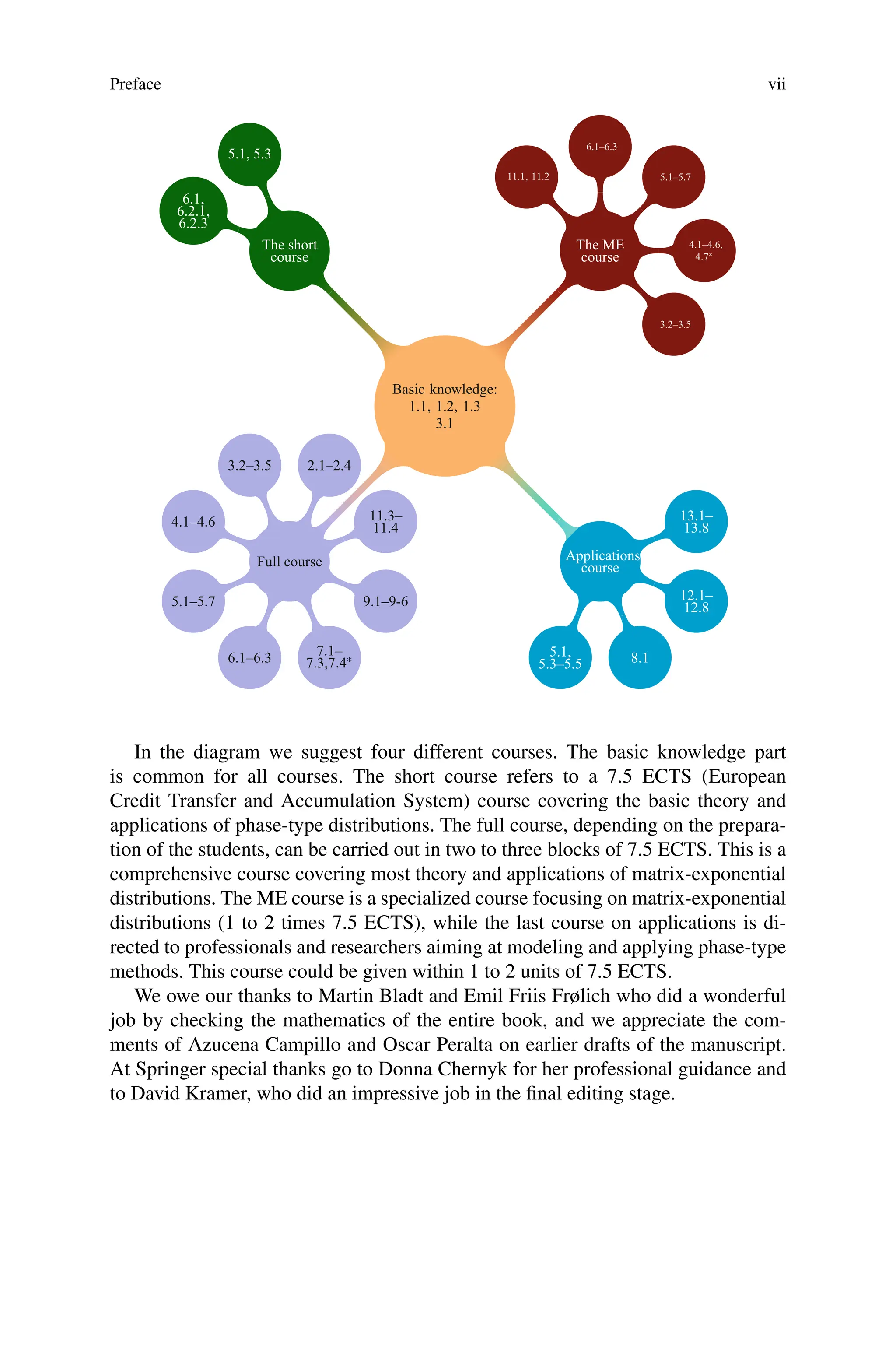

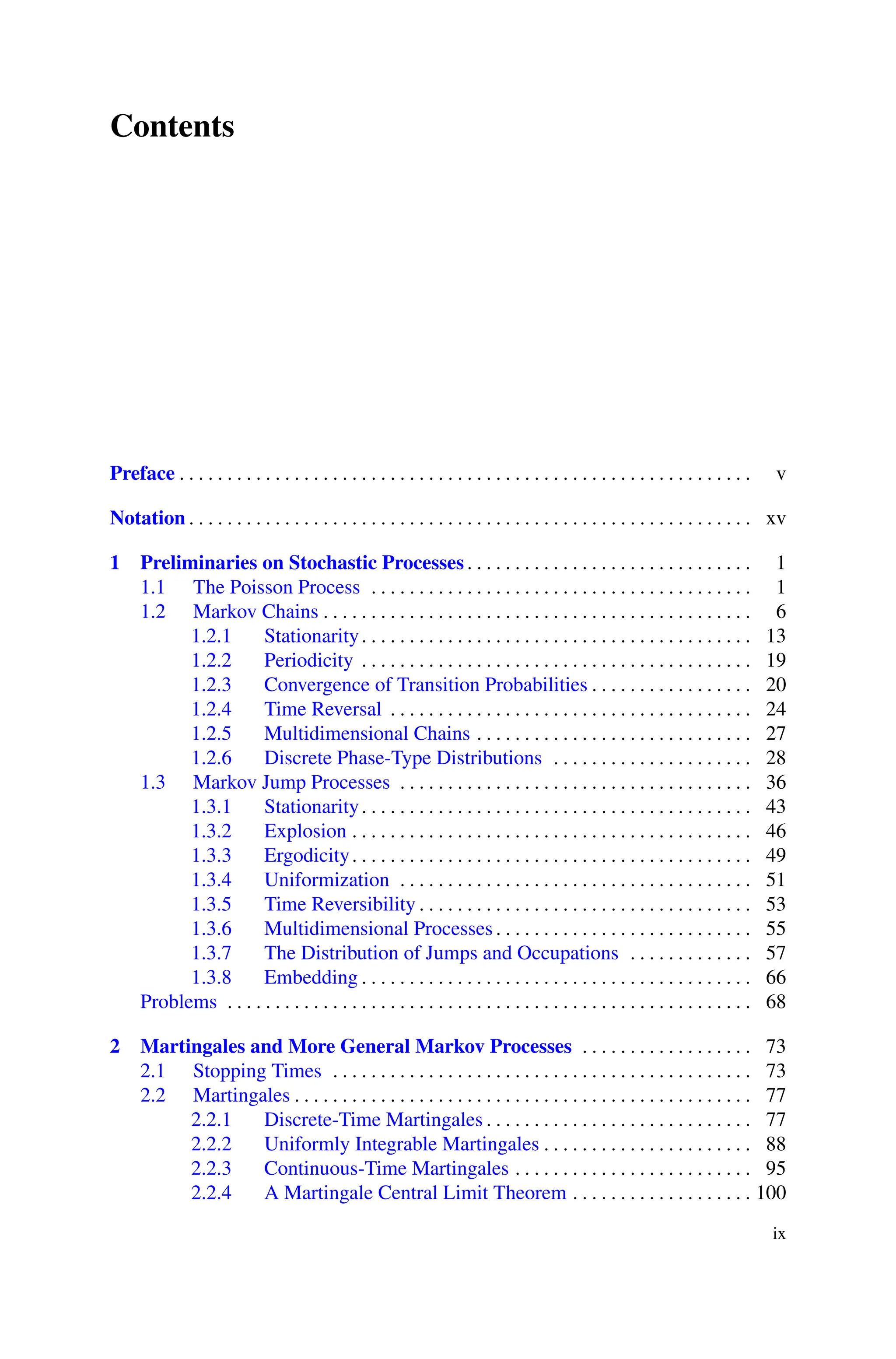
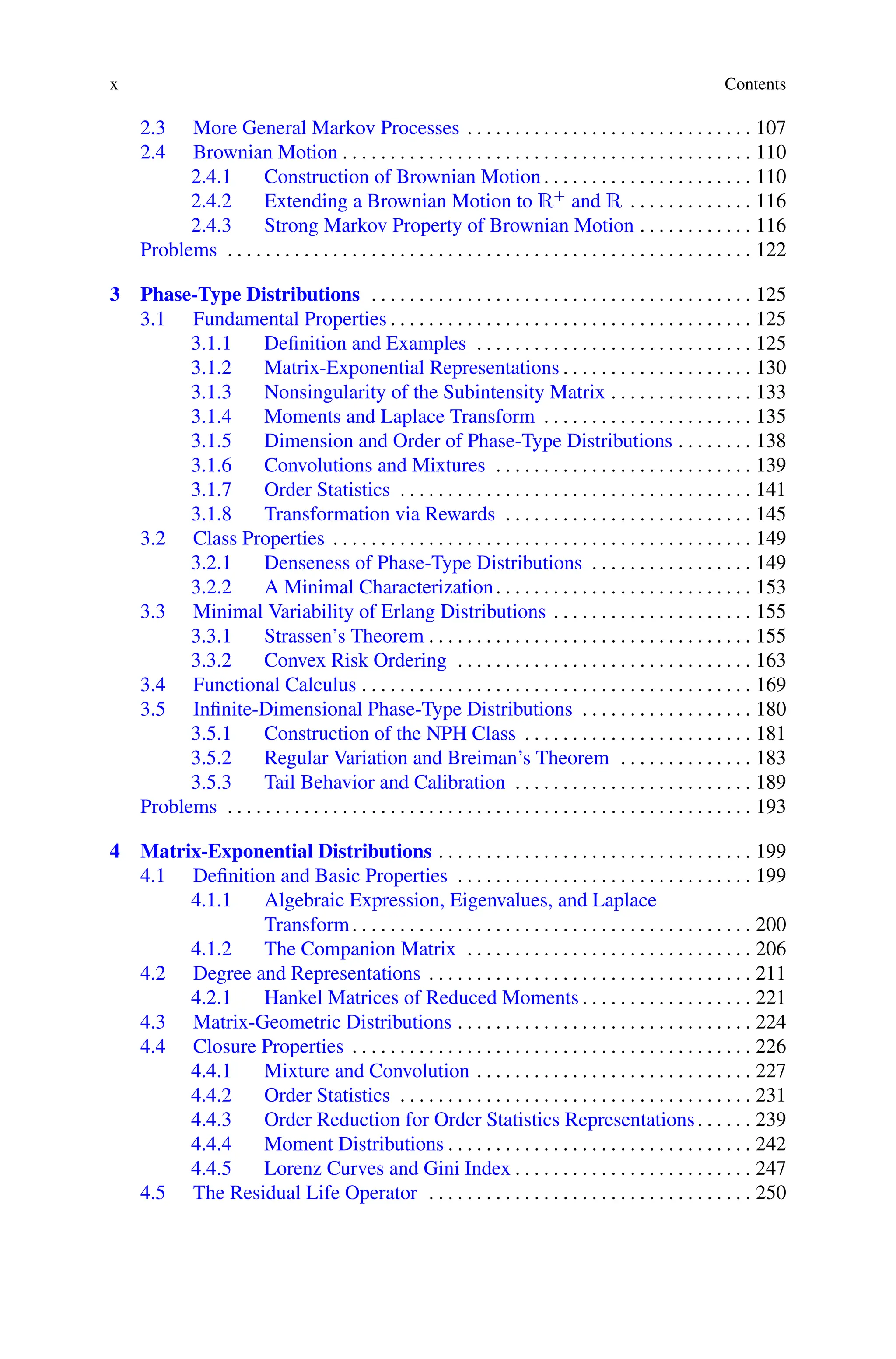
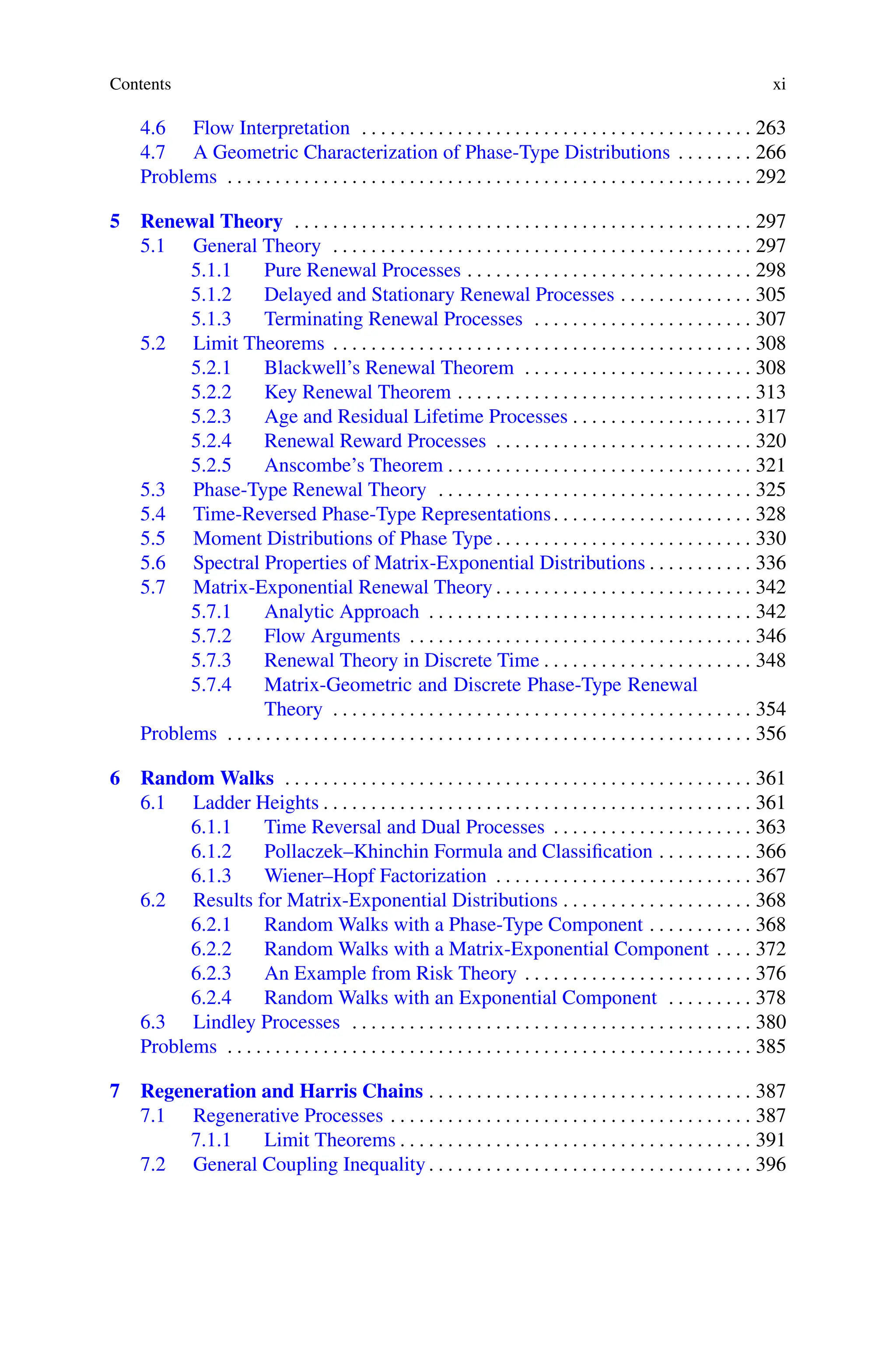
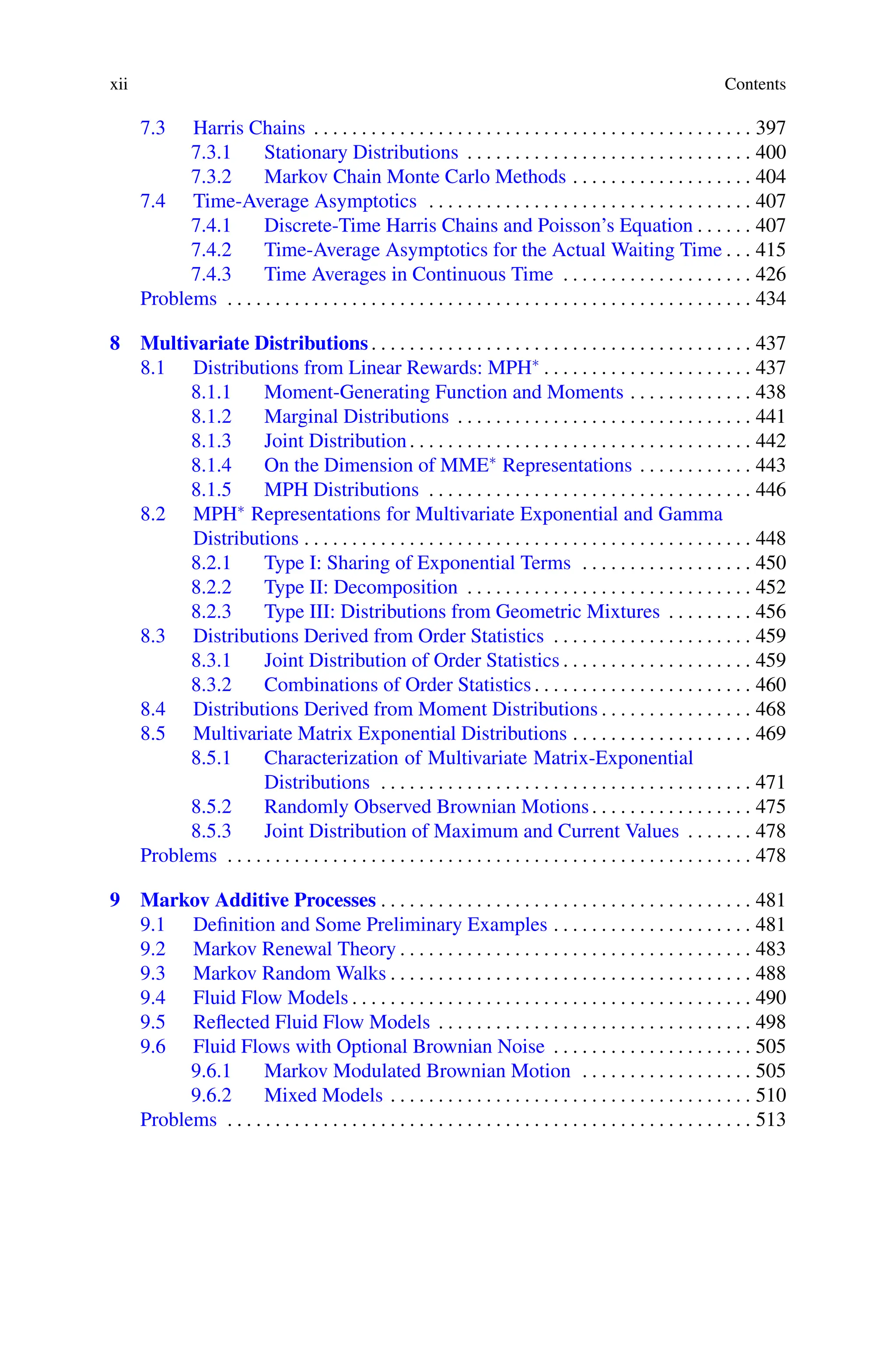
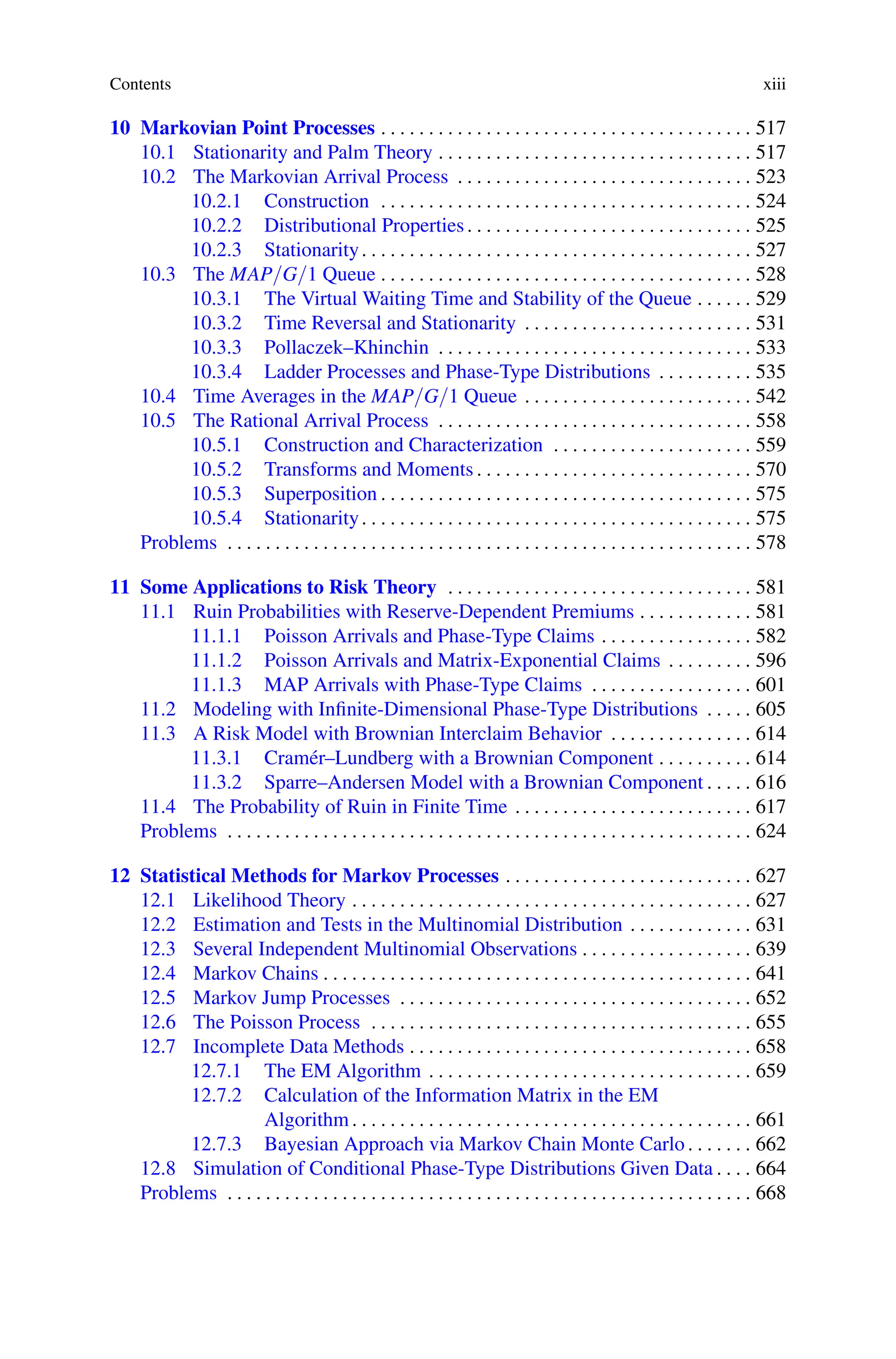
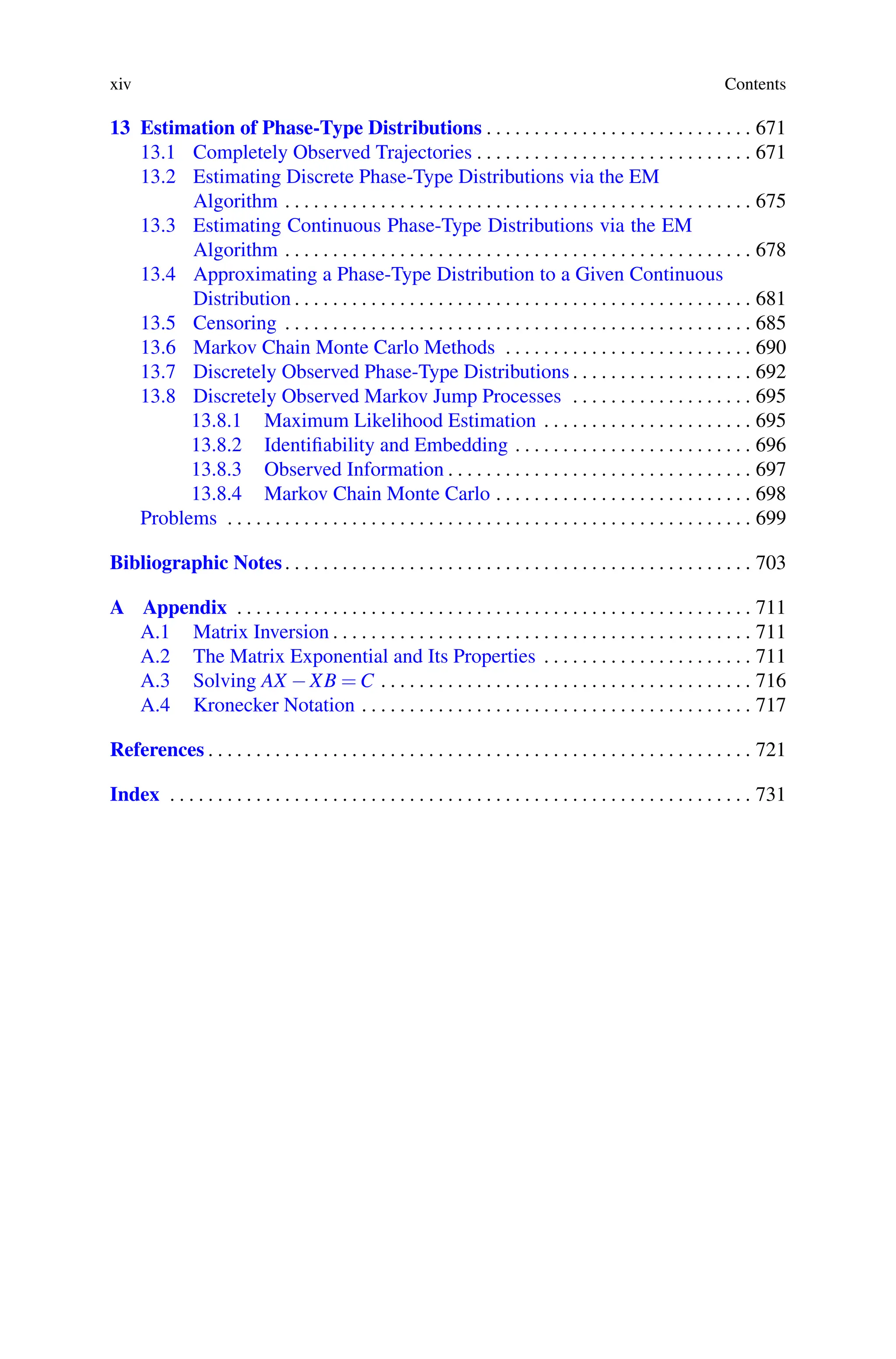
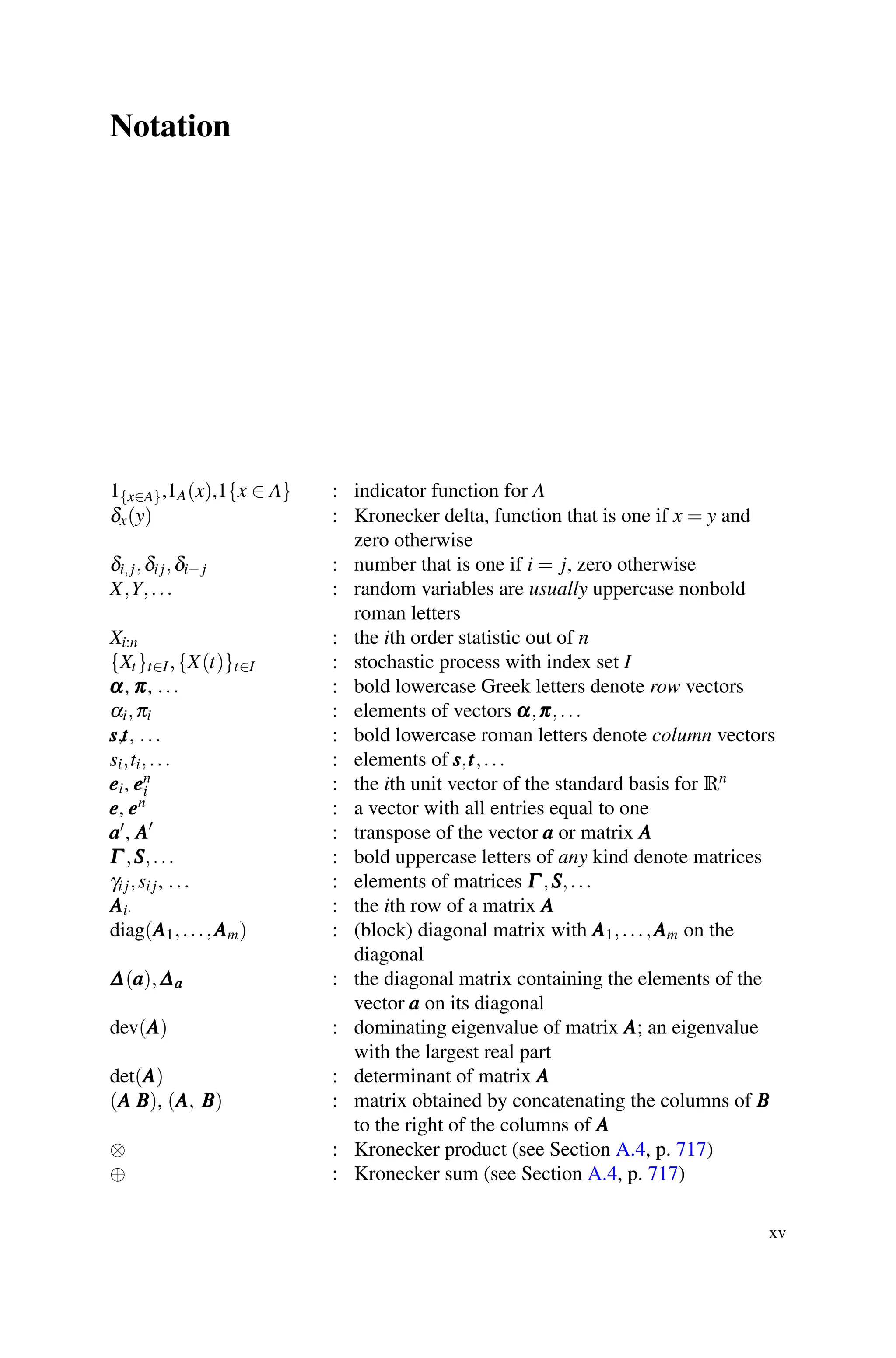
![xvi Notation
• : Schur (or Hadamard) entrywise matrix product,
{ai j}•{bi j} = {ai jbi j}
N : the natural numbers {0,1,2,...}
Z : the set of integers
Z+ : the set of positive integers {1,2,...}
R,Rn : Real numbers in one and n dimensions
C : complex numbers
int(A) : interior of a set A
Re(·), Im(·) : real and imaginary part
càdlàg : “continue à droite, limite à gauche” (right
continuous, left limits)
P : Probability (measure)
Pi : P(· | X0 = i)
E : Expectation
Var : Variance
Ei : E(· | X0 = i)
a.s. : almost surely
a.e. : almost everywhere
P
→ : convergence in probability
d
→ : convergence in distribution, weak convergence
∼,
d
= : distributed as, equality in law
a∧b, min(a,b) : minimum of a and b
a∨b, max(a,b) : maximum of a and b
a+ : positive part of a ∈ R, a = a∨0
a− : negative part of a ∈ R, a = (−a)∨0 = −a∧0
g.c.d. : greatest common divisor
[x] : integer part of x ∈ R, i.e., greatest integer less than
or equal to x
δi j : 1{i = j}, indicator for i equals j
: contour integral
I
I
I : identity matrix
E
E
Ei j : matrix with all elements equal to zero except for the
element i j, which is 1
0
0
0 : zero matrix
i.i.d. : independent identically distributed
i.n.i.d. : independent not identically distributed
LX : Laplace transform of the random variable X, i.e.,
LX (θ) = E(e−θX )
MX : moment generating function of the random variable
X, i.e., MX (θ) = E(eθX )
L ( f,θ) : Laplace transform of the function f, i.e.,
L ( f,θ) =
∞
0 e−θx f(x)dx](https://image.slidesharecdn.com/2940531-250516172746-6cfd2da3/75/Matrixexponential-Distributions-In-Applied-Probability-1st-Edition-Mogens-Bladt-21-2048.jpg)
![Chapter 1
Preliminaries on Stochastic Processes
This is an introductory chapter containing fundamental properties of Poisson
processes, Markov chains, and Markov jump processes. Apart from being of in-
terest on their own, the aforementioned topics are essential for the construction of
phase-type distributions, both discrete and continuous, as well as in applications,
stochastic modeling, and statistical methods presented in the remainder of the book.
1.1 The Poisson Process
Imagine observing the time of certain events such as cars passing a particular loca-
tion on a road or particles emitted from a radioactive source. We will refer to such
times as arrival times or simply arrivals. Let 0 S1 S2 ··· denote the arrival
times, which are random variables, and t ≥ 0, let
N(t) = sup{n ∈ N | Sn ≤ t} =
∞
∑
n=1
1{Sn ≤ t}
denote the number of arrivals observed in (0,t]. For convenience of notation we let
S0 = 0, which then implies that N(0) = 0. Then N(t) are random variables, and the
collection {N(t)}t≥0 is therefore a stochastic process. This type of process is called
a counting process, since it increases stepwise with unit increments (see Figure 1.1).
More generally, we shall use the notation
N(A) =
∞
∑
n=1
1{Sn ∈ A}
for a (measurable) set A, where N(A) counts the number of arrivals that fall into
A. Counting elements is clearly a measure (the counting measure), but since the
© Springer Science+Business Media LLC 2017
M. Bladt, B.F. Nielsen, Matrix-Exponential Distributions in Applied Probability,
Probability Theory and Stochastic Modelling 81, DOI 10.1007/978-1-4939-7049-0 1
1](https://image.slidesharecdn.com/2940531-250516172746-6cfd2da3/75/Matrixexponential-Distributions-In-Applied-Probability-1st-Edition-Mogens-Bladt-23-2048.jpg)
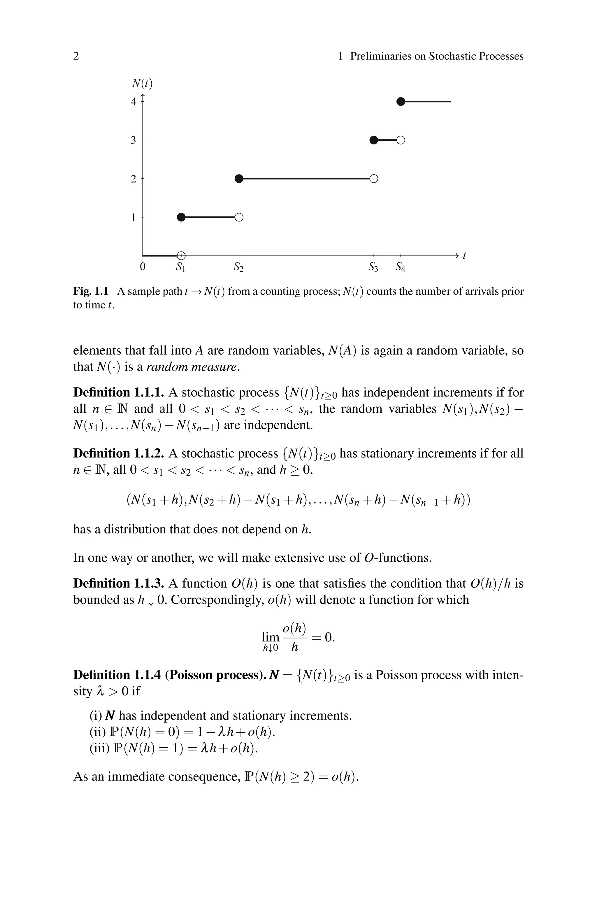
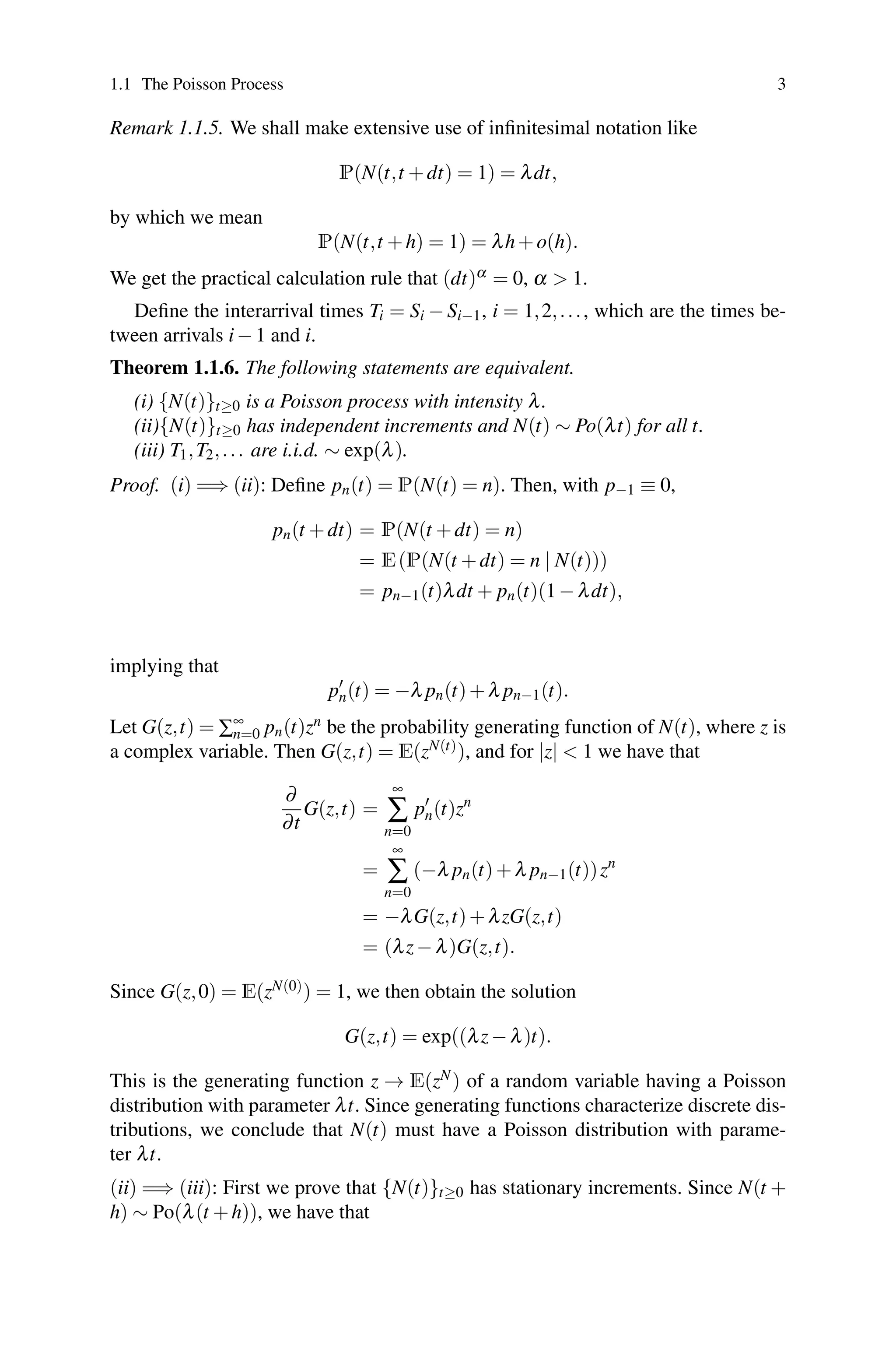
![4 1 Preliminaries on Stochastic Processes
e(λz−λ)(t+h)
= E
zN(t+h)
= E
zN(t+h)−N(h)
zN(h)
= E
zN(t+h)−N(h)
E
zN(h)
= E
zN(t+h)−N(h)
e(λz−λ)h
,
giving
E
zN(t+h)−N(h)
= e(λz−λ)t
,
from which it follows that N(t +h)−N(h) ∼ Po(λt). Hence the distribution of N(t +
h) − N(h) does not depend on h and it follows that the process also has stationary
increments.
Next we calculate the joint density f(T1,...,Tn) of the times between the first n
arrivals. Let t0 = 0 ≤ s1 t1 ≤ s2 t2 ≤ s3 t3 ≤ ··· ≤ sn tn. Then
P(sk Sk ≤ tk,k = 1,...,n)
= P(N(tk−1,sk] = 0,N(sk,tk] = 1,k = 1,...,n−1,N(tn−1,sn] = 0,N(sn,tn] ≥ 1).
There is an inequality in the last term, since the event Sn ∈ (sn,tn] does not exclude
that Sm ∈ (sn,tn] for some other m ≥ n + 1. This phenomenon does, however, not
occur in the preceding n − 1 interarrivals, since by construction, the arrivals are
positioned in disjoint intervals.
Using N(a,b) = N(b)−N(a) and the independent and stationary increments, we
get that
P(sk Sk ≤ tk,k = 1,...,n)
=
1−e−λ(tn−sn)
e−λ(sn−tn−1)
n−1
∏
k=1
λ(tk −sk)e−λ(tk−sk)
e−λ(sk−tk−1)
=
e−λsn
−e−λtn
λn−1
n−1
∏
k=1
(tk −sk).
From tn
sn
e−λx
dx =
1
λ
e−λsn
−e−λtn
,
we get that
P(sk Sk ≤ tk,k = 1,...,n) = λn
n−1
∏
k=1
(tk −sk)
tn
sn
e−λyn
dyn
=
t1
s1
···
tn−1
sn−1
tn
sn
λn
e−λyn
dyndyn−1 ···dy1.](https://image.slidesharecdn.com/2940531-250516172746-6cfd2da3/75/Matrixexponential-Distributions-In-Applied-Probability-1st-Edition-Mogens-Bladt-26-2048.jpg)
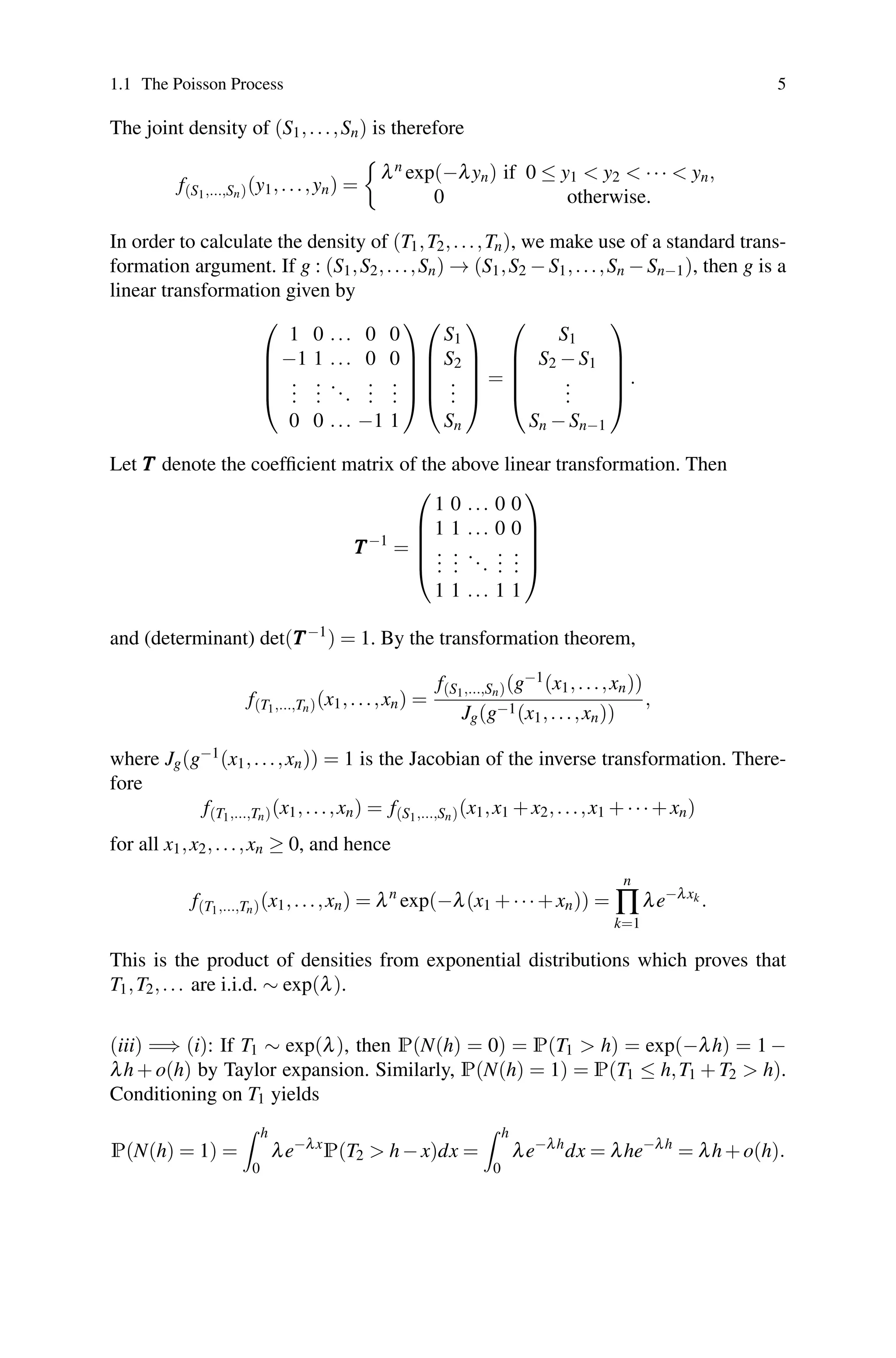
![6 1 Preliminaries on Stochastic Processes
More than one arrival in [0,h] is of order o(h), as follows directly from the two
statements above. Finally, the memoryless property of the exponential distributions
implies that the increments are both independent and stationary.
Since Sn is the sum of n independent exponentially distributed random variables
with intensity λ, we have that the density gn(x) of Sn is given by the gamma density
gn(x) = λ
(λx)n−1
(n−1)!
e−λx
for n ≥ 1. In particular, we have that
∞
∑
n=1
gn(x) = λe−λx
∞
∑
n=1
(λx)n−1
(n−1)!
= λ.
This result can be explained probabilistically in the following way. By definition of
a probability density, gn(x)dx is the probability that the nth arrival will be in [x,x+
dx). Then ∑∞
n=1 gn(x)dx is the probability that some arrival will be in [x,x+dx), but
this we already know to be equal to λdx, since it is a Poisson process.
1.2 Markov Chains
A Markov chain is a discrete-time and discrete-state-space stochastic process whose
future behavior, given its past, depends only on its present.
Definition 1.2.1. Let {Xn}n∈N = {X0,X1,X2,...} be a discrete-time stochastic pro-
cess taking values in some countable set E. Then we call {Xn}n∈N a Markov chain
with state space E if
P(Xn+1 = j | Xn = i,Xn−1 = in−1,...,X0 = i0) = P(Xn+1 = j | Xn = i) (1.1)
for all n ∈ N and all i0,...,in−1,i, j ∈ E. We refer to (1.1) as the Markov property.
The Markov chain {Xn}n∈N is said to be time-homogeneous if the probabilities
P(Xn+1 = j | Xn = i) do not depend on n. In this case, we define the (one-step)
transition probability of going from state i to state j by
pi j = P(Xn+1 = j | Xn = i).
The transition matrix P
P
P of a time-homogeneous Markov chain {Xn}n∈N is then
defined by
P
P
P = {pi j}i, j∈E.
Unless otherwise stated, we assume that all Markov chains are time-homogeneous.
Remark 1.2.2. The Markov property can be restated in terms of σ-algebras as fol-
lows. If Fn = σ(X0,X1,...,Xn) denotes the σ-algebra generated by X0,X1,...,Xn,](https://image.slidesharecdn.com/2940531-250516172746-6cfd2da3/75/Matrixexponential-Distributions-In-Applied-Probability-1st-Edition-Mogens-Bladt-28-2048.jpg)
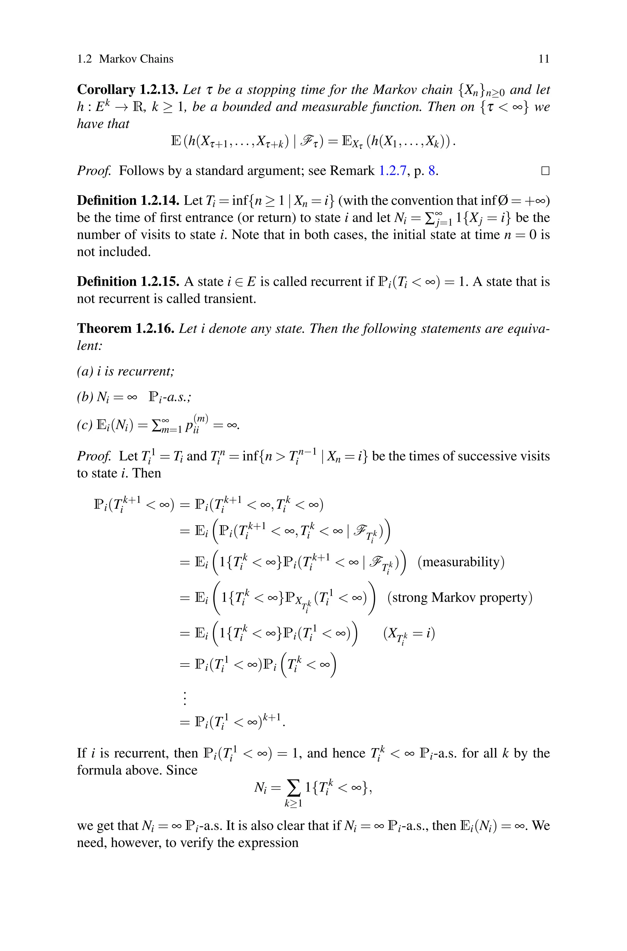
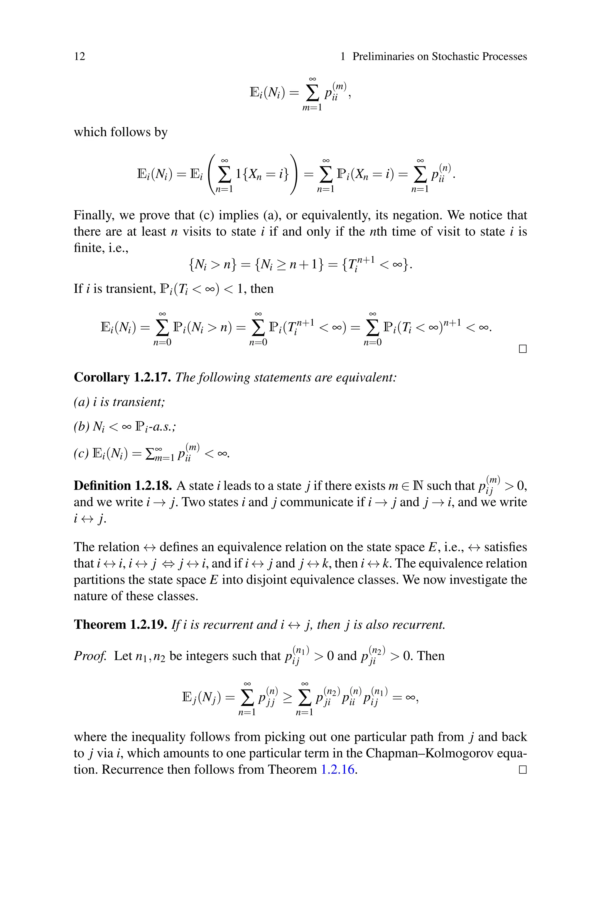
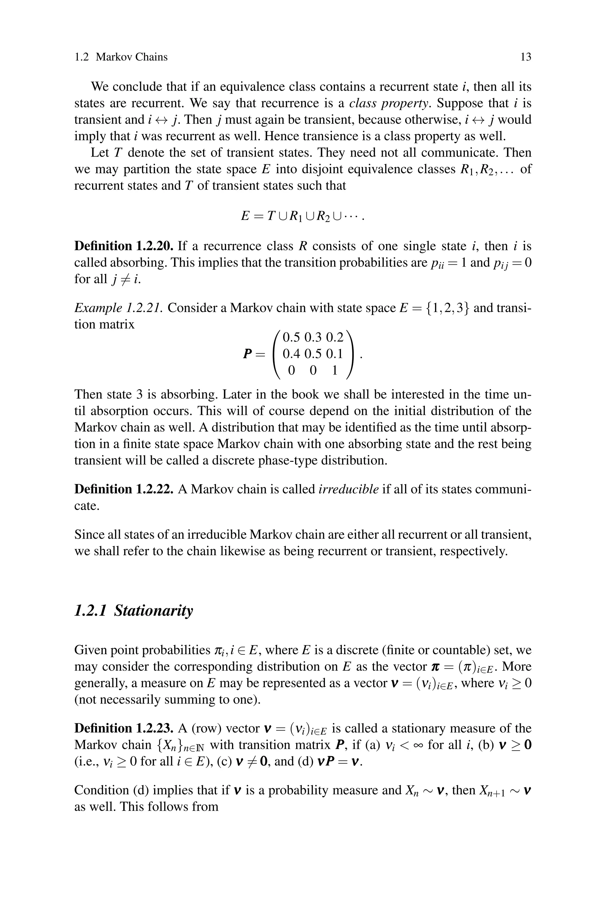
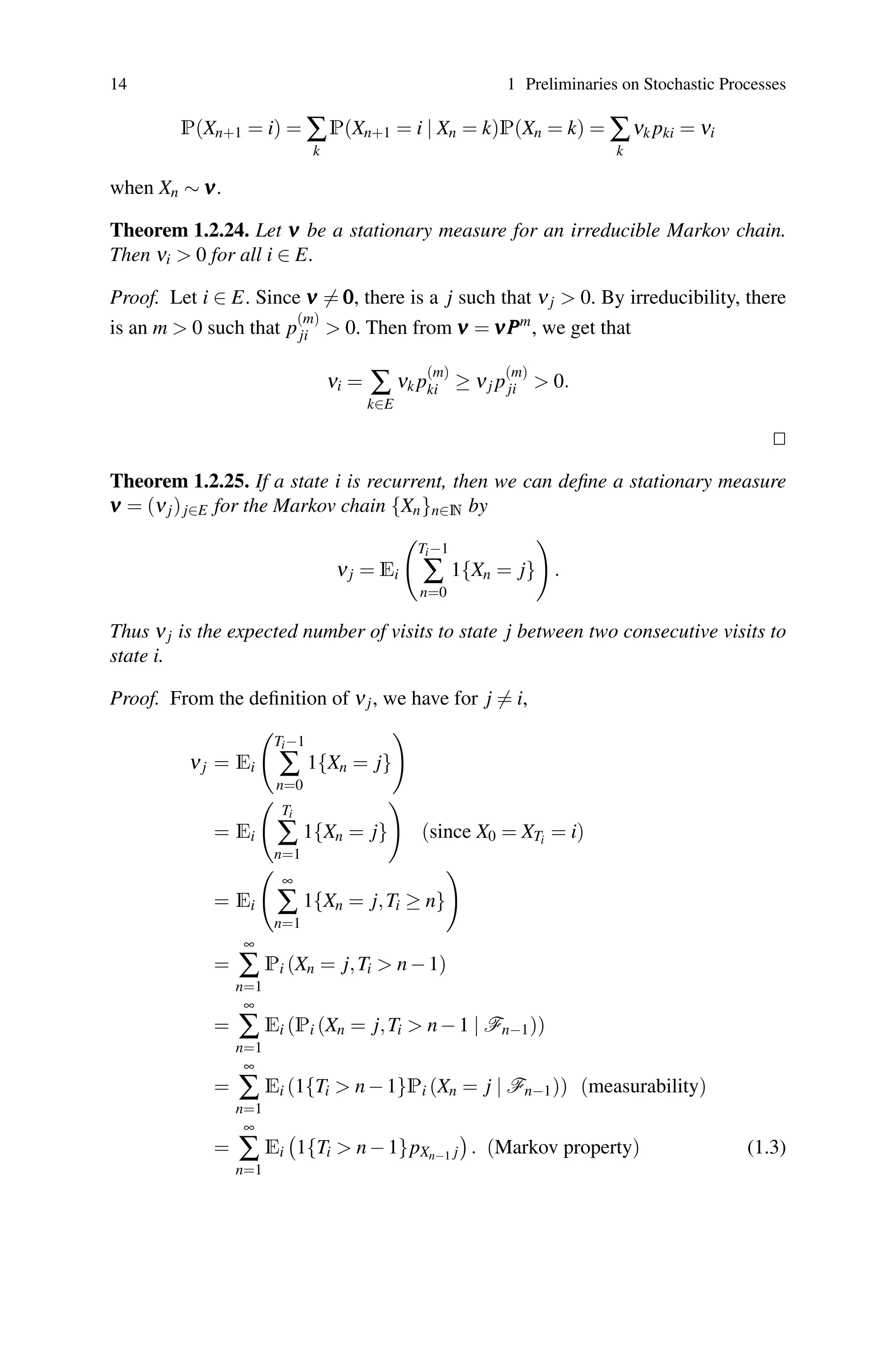

![24 1 Preliminaries on Stochastic Processes
If we consider an arbitrary m ∈ N, then m ∈ [nN,(n + 1)N] for some n = 0,1,...,
and
Pi(T̃j m) ≤ Pi(T̃j nN)
≤ (1−A)n
=
1
1−A
(1−A)1/N
)
(n+1)N
≤
1
1−A
(1−A)1/N
m
.
If we let C = 1/(1−A) and ρ = (1−A)1/N, the result of the lemma follows.
Theorem 1.2.45 (Geometric convergence rate). Let {Xn} be an ergodic Markov
chain on a finite state space E. Let π
π
π = {πi} denote its stationary distribution. Then
there are constants C 0 and 0 ρ 1 such that
p
(n)
i j −πj
≤ Cρn
, n = 1,2,... .
Proof. Consider the bivariate Markov chain on E × E defined in the proof of
Theorem 1.2.40. There it was also proved that the bivariate chain is ergodic with
stationary distribution π
π
π ⊗π
π
π. Using Lemma 1.2.44, for every pair ( j, j) we have
that
P(i,k)(T( j, j) n) ≤ Cjρn
j ,
for some constants Cj 0 and 0 ρj 1.
If T is the coupling time of the two marginals, then
T = min
j
T( j, j),
and hence
P(i,k)(T n) ≤ P(i,k)(T( j, j) n),
from which the convergence rate follows immediately by the coupling inequality.
1.2.4 Time Reversal
Time reversion plays an important role in the following chapters, and we shall here
provide a brief account of the basic construction and properties. Consider a time-
homogeneous Markov chain {Xn}n∈N with discrete state space E and transition ma-
trix P
P
P = {pi j}i, j∈E. Let N 0 be a fixed integer, and define the time-reversed process
{X̃n}n=0,...,N by
X̃i = XN−i, i = 0,1,...,N.
If P(Xn = i) 0 for all n and i ∈ E, then](https://image.slidesharecdn.com/2940531-250516172746-6cfd2da3/75/Matrixexponential-Distributions-In-Applied-Probability-1st-Edition-Mogens-Bladt-46-2048.jpg)

![prices of all manner of things, that they rule the poverty, and
oppress them at their pleasure....
“And although here I seem only to speak against these
unlawful assemblers, yet I cannot allow those, but I must
needs threaten everlasting damnation unto them, whether they
be gentlemen or whatsoever they be, which never cease to
purchase and join house to house, and land to land, as though
they alone ought to possess and inhabit the earth.”[274]
Revolt against the pressure of this unrestricted economic
competition took the form of Puritanism, of resistance to the
religious organization controlled by capital, and even in Cranmer’s
time, the attitude of the descendants of the men who formed the
line at Poitiers and Crécy was so ominous that Anglican bishops took
alarm.
“It is reported that there be many among these unlawful
assemblies that pretend knowledge of the gospel, and will
needs be called gospellers.... But now I will go further to speak
somewhat of the great hatred which divers of these seditious
persons do bear against the gentlemen; which hatred in many
is so outrageous, that they desire nothing more than the spoil,
ruin, and destruction of them that be rich and wealthy.”[275]
Somerset, who owed his elevation to the accident of being the
brother of Jane Seymour, proved unequal to the crisis of 1449, and
was supplanted by John Dudley, now better remembered as Duke of
Northumberland. Dudley was the strongest member of the new
aristocracy. His father, Edmund Dudley, had been the celebrated
lawyer who rose to eminence as the extortioner of Henry VII., and
whom Henry VIII. executed, as an act of popularity, on his
accession. John, beside inheriting his father’s financial ability, had a
certain aptitude for war, and undoubted courage; accordingly he
rose rapidly. He and Cromwell understood each other; he flattered
Cromwell, and Cromwell lent him money.[276]
Strype has intimated](https://image.slidesharecdn.com/2940531-250516172746-6cfd2da3/75/Matrixexponential-Distributions-In-Applied-Probability-1st-Edition-Mogens-Bladt-56-2048.jpg)
![that Dudley had strong motives for resisting the restoration of the
commons.[277]
In 1547 he was created Earl of Warwick, and in 1549 suppressed
Kett’s rebellion. This military success brought him to the head of the
State; he thrust Somerset aside, and took the title of Duke of
Northumberland. His son was equally distinguished. He became the
favourite of Queen Elizabeth, who created him Earl of Leicester; but,
though an expert courtier, he was one of the most incompetent
generals whom even the Tudor landed aristocracy ever put in the
field.
The disturbances of the reign of Edward VI. did not ripen into
revolution, probably because of the relief given by rising prices after
1550; but, though they fell short of actual civil war, they were
sufficiently formidable to terrify the aristocracy into abandoning their
policy of killing off the surplus population. In 1552 the first statute
was passed[278]
looking toward the systematic relief of paupers.
Small farmers prospered greatly after 1660, for prices rose strongly,
very much more strongly than rents; nor was it until after the
beginning of the seventeenth century, when rents again began to
advance, that the yeomanry once more grew restive. Cromwell
raised his Ironsides from among the great-grandchildren of the men
who stormed Norwich with Kett.
“I had a very worthy friend then; and he was a very noble
person, and I know his memory is very grateful to all,—Mr.
John Hampden. At my first going out into this engagement, I
saw our men were beaten at every hand. I did indeed; and
desired him that he would make some additions to my Lord
Essex’s army, of some new regiments; and I told him I would
be serviceable to him in bringing such men in as I thought had
a spirit that would do something in the work. This is very true
that I tell you; God knows I lie not. ‘Your troops,’ said I, ‘are
most of them old decayed serving-men, and tapsters, and such
kind of fellows; and,’ said I, ‘their troops are gentlemen’s sons,
younger sons and persons of quality: do you think that the](https://image.slidesharecdn.com/2940531-250516172746-6cfd2da3/75/Matrixexponential-Distributions-In-Applied-Probability-1st-Edition-Mogens-Bladt-57-2048.jpg)
![spirits of such base and mean fellows will ever be able to
encounter gentlemen, that have honour and courage and
resolution in them?’... Truly I did tell him; ‘You must get men of
a spirit: ... a spirit that is likely to go on as far as gentlemen
will go;—or else you will be beaten still....’
“He was a wise and worthy person; and he did think that I
talked a good notion, but an impracticable one. Truly I told him
I could do somewhat in it, ... and truly I must needs say this to
you, ... I raised such men as had the fear of God before them,
as made some conscience of what they did; and from that day
forward, I must say to you, they were never beaten, and
wherever they were engaged against the enemy, they beat
continually.”[279]
Thus, by degrees, the pressure of intensifying centralization split the
old homogeneous population of England into classes, graduated
according to their economic capacity. Those without the necessary
instinct sank into agricultural day labourers, whose lot, on the whole,
has probably been somewhat worse than that of ordinary slaves.
The gifted, like the Howards, the Dudleys, the Cecils, and the
Boleyns, rose to be rich nobles and masters of the State. Between
the two accumulated a mass of bold and needy adventurers, who
were destined finally not only to dominate England, but to shape the
destinies of the world.
One section of these, the shrewder and less venturesome, gravitated
to the towns, and grew rich as merchants, like the founder of the
Osborn family, whose descendant became Duke of Leeds; or like the
celebrated Josiah Child, who, in the reign of William III., controlled
the whole eastern trade of the kingdom. The less astute and the
more martial took to the sea, and as slavers, pirates, and
conquerors, built up England’s colonial empire, and established her
maritime supremacy. Of this class were Drake and Blake, Hawkins,
Raleigh, and Clive.
For several hundred years after the Norman conquest, Englishmen
showed little taste for the ocean, probably because sufficient outlet](https://image.slidesharecdn.com/2940531-250516172746-6cfd2da3/75/Matrixexponential-Distributions-In-Applied-Probability-1st-Edition-Mogens-Bladt-58-2048.jpg)
![use, amounted to one-tenth, or £14,000. She demanded £80,000,
and allowed Raleigh and Hawkins, who had spent £34,000, only
£36,000. Raleigh bitterly contrasted the difference made between
himself a soldier, and a peer, or a London speculator. “I was the
cause that all this came to the Queen, and that the King of Spaine
spent 300,000li
the last yere.... I that adventured all my estate, lose
of my principall.... I tooke all the care and paines; ... they only sate
still ... for which double is given to them, and less then mine own to
me.”[280]
Raleigh was so brave he could not comprehend that his talent was
his peril. He fancied his capacity for war would bring him fame and
fortune, and it led him to the block. While Elizabeth lived, the
admiration of the woman for the hero probably saved him, but he
never even entered the Privy Council, and of real power he had
none. The sovereign the oligarchy chose was James, and James
imprisoned and then slew him. Nor was Raleigh’s fate peculiar, for,
through timidity, the Cavaliers conceived an almost equal hate of
many soldiers. They dug up the bones of Cromwell, they tried to
murder William III., and they dragged down Marlborough in the
midst of victory. Such were the new classes into which economic
competition divided the people of England during the sixteenth
century, and the Reformation was only one among many of the
effects of this profound social revolution.
In the first fifty-three years of the sixteenth century, England passed
through two distinct phases of ecclesiastical reform; the earlier,
under Henry, when the conventual property was appropriated by the
rising aristocracy; the later, under Edward, when portions of the
secular endowments were also seized. Each period of spoliation was
accompanied by innovations in doctrine, and each was followed by a
reaction, the final one, under Mary, taking the form of reconciliation
with Rome. Viewed in connection with the insurrections, the whole
movement can hardly be distinguished from an armed conquest of
the imaginative by the economic section of society; a conquest
which produced a most curious and interesting development of a
new clerical type.](https://image.slidesharecdn.com/2940531-250516172746-6cfd2da3/75/Matrixexponential-Distributions-In-Applied-Probability-1st-Edition-Mogens-Bladt-61-2048.jpg)
![demand. Tradesmen, perhaps, did not easily grow rich, but they as
seldom became poor.
With centralization life changed. Competition sifted the strong from
the weak; the former waxed wealthy, and hired hands at wages, the
latter lost all but the ability to labour; and, when the corporate body
of producers had thus disintegrated, nothing stood between the
common property and the men who controlled the engine of the law.
By the 1 Edward VI., c. 14, all the possessions of the schools,
colleges, and guilds of England, except the colleges of Oxford and
Cambridge and the guilds of London, were conveyed to the king,
and the distribution thus begun extended far and wide, and has
been forcibly described by Mr. Blunt:—
“They tore off the lead from the roofs, and wrenched out the
brasses from the floors. The books they despoiled of their
costly covers, and then sold them for waste paper. The gold
and silver plate they melted down with copper and lead, to
make a coinage so shamefully debased as was never known
before or since in England. The vestments of altars and priests
they turned into table-covers, carpets, and hangings, when not
very costly; and when worth more money than usual, they sold
them to foreigners, not caring who used them for
‘superstitious’ purposes, but caring to make the best ‘bargains’
they could of their spoil. Even the very surplices and altar linen
would fetch something, and that too was seized by their
covetous hands.”[281]
These “covetous hands” were the privy councillors. Henry had not
intended that any member of the board should have precedence, but
the king’s body was not cold before Edward Seymour began an
intrigue to make himself protector. To consolidate a party behind
him, he opened his administration by distributing all the spoil he
could lay hands on; and Mr. Froude estimated that “on a
computation most favourable to the council, estates worth ... in
modern currency about five millions” of pounds, were “appropriated
—I suppose I must not say stolen—and divided among](https://image.slidesharecdn.com/2940531-250516172746-6cfd2da3/75/Matrixexponential-Distributions-In-Applied-Probability-1st-Edition-Mogens-Bladt-63-2048.jpg)
![themselves.”[282]
At the head of this council stood Cranmer, who took
his share without scruple. Probably Froude’s estimate is far too low;
for though Seymour, as Duke of Somerset, had, like Henry, to meet
imperative claims which drained his purse, he yet built Somerset
House, the most sumptuous palace of London.
Seymour was put to death by Dudley when he rose to power by his
military success in Norfolk. Dudley as well as Cromwell was fitted for
the emergency in which he lived; bold, able, unscrupulous and
energetic, his party hated but followed him, because without him
they saw no way to seize the property they coveted. He too, like
Cromwell, allied himself with the evangelical clergy, and under
Edward the orthodoxy of the “Six Articles” gave way to the doctrine
of Geneva. Even in 1548 Calvin had been able to write to Somerset,
thanking God that, through his wisdom, the “pure truth” was
preached;[283]
but when Dudley administered the government as
Duke of Northumberland, bishops did not hesitate to teach that the
dogma of the “carnal presence” in the sacrament “maintaineth that
beastly kind of cruelty of the ‘Anthropophagi,’ that is, the devourers
of man’s flesh: for it is a more cruel thing to devour a quick man,
than to slay him.”[284]
Dudley resembled Henry and Norfolk in being naturally conservative,
for he died a Catholic; but with them all, money was the supreme
object, and as they lacked the physical force to plunder alone, they
were obliged to conciliate the Radicals. These were represented by
Knox, and to Knox the duke paid assiduous court. The Scotchman
began preaching in Berwick in 1549, but the government soon
brought him to London, and in 1551 made him a royal chaplain, and,
as chaplain, he was called upon to approve the Forty-two Articles of
1552. This he could do conscientiously, as they contained the
dogmas of election and predestination, original sin, and justification
by faith, beside a denial of “the reall and bodilie presence ... of
Christes fleshe, and bloude, in the Sacramente of the Lordes
Supper.”](https://image.slidesharecdn.com/2940531-250516172746-6cfd2da3/75/Matrixexponential-Distributions-In-Applied-Probability-1st-Edition-Mogens-Bladt-64-2048.jpg)
![Dudley tried hard to buy Knox, and offered him the See of
Rochester; but the duke excited the deepest distrust and dislike in
the preacher, who called him “that wretched and miserable
Northumberland.” He rejected the preferment, and indeed, from the
beginning, bad blood seems to have lain between the Calvinists and
the court. Writing at the beginning of 1554, Knox expressed his
opinion of the reforming aristocracy in emphatic language, beginning
with Somerset, “who became so cold in hearing Godis Word, that the
year befoir his last apprehensioun, he wald ga visit his masonis, and
wald not dainyie himself to ga frome his gallerie to his hall for
heiring of a sermone.”[285]
Afterward matters grew worse, for “the
haill Counsaile had said, Thay wald heir no mo of thair sermonis:
thay wer but indifferent fellowis; (yea, and sum of thame eschameit
not to call thame pratting knaves.)”[286]
Finally, just before Edward’s death the open rupture came. Knox had
a supreme contempt and antipathy for the Lord Treasurer, Paulet,
Marquis of Winchester, whom he called a “crafty fox.” During
Edward’s life, jeered Knox, “who was moste bolde to crye, Bastarde,
bastarde, incestuous bastarde, Mary shall never rule over us,” and
now that Mary is on the throne it is to her Paulet “crouches and
kneeleth.”[287]
In the last sermon he preached before the king he let
loose his tongue, and probably he would have quitted the court,
even had the reign continued. In this sermon Dudley was
Ahithophel, Paulet, Shebna:—
“I made this affirmacion, That commonlye it was sene, that the
most godly princes hadde officers and chief counseilours moste
ungodlye, conjured enemies to Goddes true religion, and
traitours to their princes.... Was David, sayd I, and Ezechias,
princes of great and godly giftes and experience, abused by
crafty counsailers and dissemblyng hypocrites? What wonder is
it then, that a yonge and innocent Kinge be deceived by
craftye, covetouse, wycked, and ungodly counselours? I am
greatly afrayd, that Achitophel be counsailer, that Judas beare
the purse, and that Sobna be scribe, comptroller, and treasurer.](https://image.slidesharecdn.com/2940531-250516172746-6cfd2da3/75/Matrixexponential-Distributions-In-Applied-Probability-1st-Edition-Mogens-Bladt-65-2048.jpg)
![This, and somwhat more I spake that daye, not in a corner (as
many yet can wytnesse) but even before those whome my
conscience judged worthy of accusation.”[288]
Knox understood the relation which men of his stamp bore to
Anglicanism. In 1549 much land yet remained to be divided,
therefore he and his like were flattered and cajoled until Paulet and
his friends should be strong enough to discard them. Faith, in the
hands of the monied oligarchy, became an instrument of police, and,
from the Reformation downward, revelation has been expounded in
England by statute. Hence men of the imaginative type, who could
not accept their creed with their stipend, were at any moment in
danger of being adjudged heretics, and suffering the extreme
penalty of insubordination.
Docility to lay dictation has always been the test by which the
Anglican clergy have been sifted from Catholics and Puritans. To the
imaginative mind a faith must spring from a revelation, and a
revelation must be infallible and unchangeable. Truth must be single.
Catholics believed their revelation to be continuous, delivered
through the mouth of an illuminated priesthood, speaking in its
corporate capacity. Puritans held that theirs had been made once for
all, and was contained in a book. But both Catholics and Puritans
were clear that divine truth was immutable, and that the universal
Church could not err. To minds of this type, statutes regulating the
appearance of God’s body in the elements were not only impious but
absurd, and men of the priestly temperament, whether Catholic or
Puritan, have faced death in its most appalling forms, rather than
bow down before them.
Here Fisher and Knox, Bellarmine and Calvin, agreed. Rather than
accept the royal supremacy, the flower of the English priesthood
sought poverty and exile, the scaffold and the stake. For this, the
aged Fisher hastened to the block on Tower Hill; for this, Forest
dangled over the embers of the smouldering rood; for this, the
Carthusians rotted in their noisome dens. Nor were Puritans a whit
behind Catholics in asserting the sacerdotal dignity; “Erant enim](https://image.slidesharecdn.com/2940531-250516172746-6cfd2da3/75/Matrixexponential-Distributions-In-Applied-Probability-1st-Edition-Mogens-Bladt-66-2048.jpg)
![blasphemi qui vocarent eum [Henricum VIII.] summum caput
ecclesiæ sub Christo,” wrote Calvin, and on this ground the
Nonconformists fought the established Church, from Elizabeth’s
accession downward.
The writings of Martin Marprelate only restated an issue which had
been raised by Hildebrand five hundred years before; for the
advance of centralization had reproduced in England something of
the same conditions which prevailed at Constantinople when it
became a centre of exchanges. Wherever civilization has reached
the point at which energy expresses itself through money, faith must
be subordinate to the representative of wealth. Stephen Gardiner
understood the conditions under which he lived, and accepted his
servitude in consideration of the great See of Winchester. With
striking acuteness he cited Justinian as a precedent for Henry:—
“Then, Sir, who did ever disallow Justinian’s fact, that made
laws concerning the glorious Trinity, and the Catholic faith, of
bishops, of men, of the clergy, of heretics, and others, such
like?”[289]
From the day of the breach with Rome, the British priesthood sank
into wage-earners, and those of the ancient clergy who remained in
the Anglican hierarchy after the Reformation, acquiesced in their
position, as appeared in all their writings, but in none, perhaps,
more strikingly than in the Formularies of Faith of Henry VIII., where
the episcopal bench submitted their views of orthodoxy to the
revision of the secular power:—
“And albeit, most dread and benign sovereign lord, we do
affirm by our learnings with one assent, that the said treatise is
in all points so concordant and agreeable to holy scripture, as
we trust your majesty shall receive the same as a thing most
sincerely and purely handled, to the glory of God, your grace’s
honour, the unity of your people, the which things your
highness, we may well see and perceive, doth chiefly in the
same desire: yet we do most humbly submit it to the most](https://image.slidesharecdn.com/2940531-250516172746-6cfd2da3/75/Matrixexponential-Distributions-In-Applied-Probability-1st-Edition-Mogens-Bladt-67-2048.jpg)
![excellent wisdom and exact judgment of your majesty, to be
recognised, overseen, and corrected, if your grace shall find
any word or sentence in it meet to be changed, qualified, or
further expounded, for the plain setting forth of your
highness’s most virtuous desire and purpose in that behalf.
Whereunto we shall in that case conform ourselves, as to our
most bounden duties to God and to your highness
appertaineth.”
Signed by “your highness’ most humble subjects and daily
beadsmen, Thomas Cantuarien” and all the bishops.[290]
A Church thus lying at the mercy of the temporal power, became a
chattel in the hands of the class which controlled the revenue, and,
from the Reformation to the revolution of 1688, this class consisted
of a comparatively few great landed families, forming a narrow
oligarchy which guided the Crown. In the Middle Ages, a king had
drawn his army from his own domain. Cœur-de-Lion had his own
means of attack and defence like any other baron, only on a larger
scale. Henry VIII., on the contrary, stood alone and helpless. As
centralization advanced, the cost of administration grew, until
regular taxation had become necessary, and yet taxes could only be
levied by Parliament. The king could hardly pay a body-guard, and
such military force as existed within the realm obeyed the landlords.
Had it not been for a few opulent nobles, like Norfolk and
Shrewsbury, the Pilgrims of Grace might have marched to London
and plucked Henry from his throne, as easily as William afterward
plucked James. These landlords, together with the London
tradesmen, carried Henry through the crisis of 1536, and thereafter
he lay in their hands. His impotence appeared in every act of his
reign. He ran the risk and paid the price, while others fattened on
the plunder. The Howards, the Cecils, the Russells, the Dudleys,
divided the Church spoil among themselves, and wrung from the
Crown its last penny, so that Henry lived in debt, and Edward faced
insolvency.](https://image.slidesharecdn.com/2940531-250516172746-6cfd2da3/75/Matrixexponential-Distributions-In-Applied-Probability-1st-Edition-Mogens-Bladt-68-2048.jpg)
![Deeply as Mary abhorred sacrilege, she dared not ask for restitution
to the abbeys. Such a step would probably have caused her
overthrow, while Elizabeth never attempted opposition, but obeyed
Cecil, the incarnation of the spirit of the oligarchy. The men who
formed this oligarchy were of totally different type from anything
which flourished in England in the imaginative age. Unwarlike, for
their insular position made it possible for them to survive without the
martial quality, they always shrank from arms. Nor were they
numerous enough, or strong enough, to overawe the nation even in
quiet times. Accordingly they generally lay inert, and only from
necessity allied themselves with some more turbulent faction.
The Tudor aristocracy were rich, phlegmatic, and unimaginative
men, in whom the other faculties were subordinated to acquisition,
and they treated their religion as a financial investment. Strictly
speaking, the Church of England never had a faith, but vibrated
between the orthodoxy of the “Six Articles,” and the Calvinism of the
“Lambeth Articles,” according to the exigencies of real estate. Within
a single generation, the relation Christ’s flesh and blood bore to the
bread and wine was changed five times by royal proclamation or act
of Parliament.
But if creeds were alike to the new economic aristocracy, it well
understood the value of the pulpit as a branch of the police of the
kingdom, and from the outset it used the clergy as part of the
secular administration. On this point Cranmer was explicit.[291]
Elizabeth probably represented the landed gentry more perfectly
than any other sovereign, and she told her bishops plainly that she
cared little for doctrine, but wanted clerks to keep order. She
remarked that she had seen it said:—
“that hir Protestants themselves misliked hir, and in deede so
they doe (quoth she) for I have heard that some of them of
late have said, that I was of no religion, neither hot nor cold,
but such a one, as one day would give God the vomit.... After
this she wished the bishops to look unto private Conventicles,
and now (quoth she) I miss my Lord of London who looketh no](https://image.slidesharecdn.com/2940531-250516172746-6cfd2da3/75/Matrixexponential-Distributions-In-Applied-Probability-1st-Edition-Mogens-Bladt-69-2048.jpg)
![better unto the Citty where every merchant must have his
schoolemaster and nightly conventicles.” [292]
Elizabeth ruled her clergy with a rod of iron. No priest was allowed
to marry without the approbation of two justices of the peace,
beside the bishop, nor the head of a college without the leave of the
visitor. When the Dean of St. Paul’s offended the queen in his
sermon, she told him “to retire from that ungodly digression and
return to his text,” and Grindall was suspended for disobedience to
her orders.
In Grindall’s primacy, monthly prayer meetings, called
“prophesyings,” came into fashion among the clergy. For some
reason these meetings gave the government offence, and Grindall
was directed to put a stop to them. Attacked thus, in the priests’
dearest rights, the archbishop refused. Without more ado the old
prelate was suspended, nor was he pardoned until he made
submission five years later.
The correspondence of the Elizabethan bishops is filled with
accounts of their thraldom. Pilkington, among others, complained
that “We are under authority, and cannot make any innovation
without the sanction of the queen ... and the only alternative now
allowed us is, whether we will bear with these things or disturb the
peace of the Church.”[293]
Even ecclesiastical property continued to be seized, where it could
be taken safely; and the story of Ely House, although it has been
denied, is authentic in spirit. From the beginning of the Reformation
the London palaces of the bishops had been a tempting prize. Henry
took York House for himself, Raleigh had a lease of Durham House,
and, about 1565, Sir Christopher Hatton, whose relations with the
queen were hardly equivocal, undertook to force Bishop Cox to
convey him Ely House. The bishop resisted. Hatton applied to the
queen, and she is said to have cut the matter short thus:—
“Proud prelate: I understand you are backward in complying
with your agreement, but I would have you know that I who](https://image.slidesharecdn.com/2940531-250516172746-6cfd2da3/75/Matrixexponential-Distributions-In-Applied-Probability-1st-Edition-Mogens-Bladt-70-2048.jpg)
![made you what you are can unmake you, and if you do not
forthwith fulfil your engagement, by God, I will immediately
unfrock you. Elizabeth.”
Had the great landlords been either stronger, so as to have
controlled the blouse of Commons, or more military, so as to have
suppressed it, English ecclesiastical development would have been
different. As it was, a knot of ruling families, gorged with plunder, lay
between the Catholics and the more fortunate of the evicted
yeomen, who had made money by trade, and who hated and
competed with them. Puritans as well as Catholics sought to unsettle
titles to Church lands:—
“It is wonderfull to see how dispitefully they write of this
matter. They call us church robbers, devourers of holly things,
cormorantes, etc. affirminge that by the lawe of god, things
once consecrated to god for the service of this churche, belong
unto him for ever.... ffor my owne pte I have some
imppriations, etc. I thanke god I keepe them wth
a good
conscience, and many wold be ondone. The law appveth
us.”[294]
Thus beset, the landed capitalists struggled hard to maintain
themselves, and, as their best defence, they organized a body of
priests to preach and teach the divine right of primogeniture, which
became the distinctive dogma of this national church. Such at least
was the opinion of the non-jurors, who have always ranked among
the most orthodox of the Anglican clergy, and who certainly were all
who had the constancy to suffer for their faith. John Lake, Bishop of
Chichester, suspended in 1689 for not swearing allegiance to William
and Mary, on his death-bed made the following statement:—
“That whereas I was baptized into the religion of the Church of
England, and sucked it in with my milk, I have constantly
adhered to it through the whole course of my life, and now, if
so be the will of God, shall dye in it; and I had resolved](https://image.slidesharecdn.com/2940531-250516172746-6cfd2da3/75/Matrixexponential-Distributions-In-Applied-Probability-1st-Edition-Mogens-Bladt-71-2048.jpg)
![through God’s grace assisting me to have dyed so, though at a
stake.
“And whereas that religion of the Church of England taught me
the doctrine of non-resistance and passive obedience, which I
have accordingly inculcated upon others, and which I took to
be the distinguishing character of the Church of England, I
adhere no less firmly and steadfastly to that, and in
consequence of it, have incurred a suspension from the
exercise of my office and expected a deprivation.”[295]
In the twelfth century, the sovereign drew his supernatural quality
from his consecration by the priesthood; in the seventeenth century,
money had already come to represent a force so predominant that
the process had become reversed, and the priesthood attributed its
prerogative to speak in the name of the Deity, to the interposition of
the king. This was the substance of the Reformation in England.
Cranmer taught that God committed to Christian princes “the whole
cure of all their subjects, as well concerning the administration of
God’s word ... as ... of things political”; therefore bishops, parsons,
and vicars were ministers of the temporal ruler, to whom he confided
the ecclesiastical office, as he confided the enforcement of order to a
chief of police.[296]
As a part of the secular administration, the main
function of the Reformed priesthood was to preach obedience to
their patrons; and the doctrine they evolved has been thus summed
up by Macaulay:—
“It was gravely maintained that the Supreme Being regarded
hereditary monarchy, as opposed to other forms of
government, with peculiar favour; that the rule of succession in
order of primogeniture was a divine institution, anterior to the
Christian, and even to the Mosaic dispensation; that no human
power ... could deprive a legitimate prince of his rights; that
the authority of such a prince was necessarily always
despotic....”[297]](https://image.slidesharecdn.com/2940531-250516172746-6cfd2da3/75/Matrixexponential-Distributions-In-Applied-Probability-1st-Edition-Mogens-Bladt-72-2048.jpg)
![In no other department of public affairs did the landed gentry show
particular energy or ability. Their army was ineffective, their navy
unequal to its work, their finances indifferently handled, but down to
the time of their overthrow, in 1688, they were eminently successful
in ecclesiastical organization. They chose their instruments with
precision, and an oligarchy has seldom been more adroitly served.
Macaulay was a practical politician, and Macaulay rated the clergy as
the chief political power under Charles II:—
“At every important conjuncture, invectives against the Whigs
and exhortations to obey the Lord’s anointed resounded at
once from many thousands of pulpits; and the effect was
formidable indeed. Of all the causes which, after the
dissolution of the Oxford Parliament, produced the violent
reaction against the exclusionists, the most potent seems to
have been the oratory of the country clergy.”[298]
For country squires a wage-earning clergy was safe, and although
Macaulay’s famous passage describing their fear of an army has met
with contradiction, it probably is true:—
“In their minds a standing army was inseparably associated
with the Rump, with the Protector, with the spoliation of the
Church, with the purgation of the Universities, with the
abolition of the peerage, with the murder of the King, with the
sullen reign of the Saints, with cant and asceticism, with fines
and sequestrations, with the insults which Major Generals,
sprung from the dregs of the people, had offered to the oldest
and most honourable families of the kingdom. There was,
moreover, scarcely a baronet or a squire in the parliament who
did not owe part of his importance in his own county to his
rank in the militia. If that national force were set aside, the
gentry of England must lose much of their dignity and
influence.”[299]
The work to be done by the Tudor hierarchy was mercenary, not
imaginative; therefore pastors had to be chosen who could be](https://image.slidesharecdn.com/2940531-250516172746-6cfd2da3/75/Matrixexponential-Distributions-In-Applied-Probability-1st-Edition-Mogens-Bladt-73-2048.jpg)
![trusted to labour faithfully for wages. Perhaps no equally large and
intelligent body of men has ever been more skilfully selected. The
Anglican priests, as a body, have uniformly been true to the hand
which fed them, without regard to the principles they were required
to preach. A remarkable instance of their docility, where loss of
income was the penalty for disobedience, was furnished at the
accession of William and Mary. Divine right was, of course, the most
sacred of Anglican dogmas, and yet, when the clergy were
commanded to take the oath of allegiance to him whom they held to
be an usurper, as Macaulay has observed, “some of the strongest
motives which can influence the human mind, had prevailed. Above
twenty-nine thirtieths of the profession submitted to the law.”[300]
Moreover, the landlords had the economic instinct, bargaining
accordingly, and Elizabeth bluntly told her bishops that they must
get her sober, respectable preachers, but men who should be cheap.
“Then spake my Lord Treasurer.... Her Maty hath declared unto
you a marvellous great fault, in that you make in this time of
light so many lewd and unlearned ministers.... It is the Bishop
of Litchfield ... that I mean, who made LXX. ministers in one
day for money, some taylors, some shoemakers, and other
craftsmen, I am sure the greatest part of them not worthy to
keep horses. Then said the Bp. of Rochester, that may be so,
for I know one that made 7 in one day, I would every man
might beare his own burthen, some of us have the greatest
wrong that can be offred.... But my Lord, if you would have
none but learned preachers to be admitted into the ministery,
you must provide better livings for them....
“To have learned ministers in every parish is in my judgmt
impossible (quoth my Ld. of Canterbury) being 13,000 parishes
in Ingland, I know not how this realm should yield so many
learned preachers.
“Jesus (quoth the Queen) 13,000 it is not to be looked for, I
thinke the time hath been, there hath not been 4. preachers in
a diocesse, my meaning is not you should make choice of](https://image.slidesharecdn.com/2940531-250516172746-6cfd2da3/75/Matrixexponential-Distributions-In-Applied-Probability-1st-Edition-Mogens-Bladt-74-2048.jpg)
![learned ministers only for they are not to be found, but of
honest, sober, and wise men, and such as can reade the
scriptures and homilies well unto the people.”[301]
The Anglican clergy under the Tudors and the Stuarts were not so
much priests, in the sense of the twelfth century, as hired political
retainers. Macaulay’s celebrated description is too well known to
need full quotation: “for one who made the figure of a gentleman,
ten were mere menial servants.... The coarse and ignorant squire”
could hire a “young Levite” for his board, a small garret, and ten
pounds a year. This clergyman “might not only be the most patient
of butts and of listeners, might not only be always ready in fine
weather for bowls, and in rainy weather for shovelboard, but might
also save the expense of a gardener, or of a groom. Sometimes the
reverend man nailed up the apricots; and sometimes he curried the
coach horses.”[302]
Yet, as Macaulay has also pointed out, the hierarchy was divided into
two sections, the ordinary labourers and the managers. The latter
were indispensable to the aristocracy, since without them their
machine could hardly have been kept in motion, and these were
men of talent who demanded and received good wages. Probably for
this reason a large revenue was reserved for the higher secular
clergy, and from the outset the policy proved successful. Many of the
ablest organizers and astutest politicians of England, during the
sixteenth and seventeenth centuries, sat on the episcopal bench,
and two of the most typical, as well as the ablest Anglicans who ever
lived, were the two eminent bishops who led the opposing wings of
the Church when it was reformed by Henry VIII.: Stephen Gardiner
and Thomas Cranmer.
Gardiner was the son of a clothworker of Bury Saint Edmunds, and
was born about 1483. At Cambridge he made himself the best civil
lawyer of the kingdom, and on meeting Wolsey, so strongly
impressed him with his talent that the cardinal advanced him rapidly,
and in January 1529 sent him to negotiate for the divorce at Rome.
Nobody doubts that to the end of his life Gardiner remained a](https://image.slidesharecdn.com/2940531-250516172746-6cfd2da3/75/Matrixexponential-Distributions-In-Applied-Probability-1st-Edition-Mogens-Bladt-75-2048.jpg)
![sincere Catholic, but above all else he was a great Anglican.
Becoming secretary to the king in June, 1529, as Wolsey was
tottering to his fall, he laboured to bring the University of Cambridge
to the royal side, and he also devoted himself to Anne until he
obtained the See of Winchester, when his efforts for the divorce
slackened. He even went so far as to assure Clement that he had
repented, and meant to quit the court, but notwithstanding he “bore
up the laps” of Anne’s robe at her coronation.
In 1535 the ways parted, a decision could not be deferred, he
renounced Rome and preached his sermon “de vera Obedientia,” in
which he recognized in Henry the supremacy of a Byzantine
emperor. The pang this act cost him lasted till he died, and he told
the papal nuncio “he made this book under compulsion, not having
the strength to suffer death patiently, which was ready for him.”[303]
Indeed, when dying, his apostacy seems to have been his last
thought, for in his closing hours, as the story of the passion was
read to him he exclaimed, “Negavi cum Petro, exivi cum Petro, sed
nondum flevi cum Petro.” All his life long his enemies accused him of
dissimulation and hypocrisy for acts like these, but it was precisely
this quality which raised him to eminence. Had he not been
purchasable, he could hardly have survived as an Anglican bishop;
an enthusiast like Fisher would have ended on Tower Hill.
Perhaps more fully than any other prelate of his time, Gardiner
represented the faction of Henry and Norfolk; he was as orthodox as
he could be and yet prosper. He hated Cromwell and all “gospellers,”
and he loved power and splendour and office. Fisher, with the
temperament of Saint Anselm, shivering in his squalid house, clad in
his shirt of hair, and sleeping on his pallet of straw, might indeed
“humbly thank the king’s majesty” who rid him of “all this worldly
business,” but men who rose to eminence in the reformed church
were made of different stuff, and Gardiner’s ruling passion never
burned more fiercely than as he neared his death. Though in
excruciating torments from disease, he clung to office to the last.
Noailles, the French ambassador, at a last interview, found him “livid
with jaundice and bursting with dropsy: but for two hours he held](https://image.slidesharecdn.com/2940531-250516172746-6cfd2da3/75/Matrixexponential-Distributions-In-Applied-Probability-1st-Edition-Mogens-Bladt-76-2048.jpg)
![discourse with me calmly and graciously, without a sign of
discomposure; and at parting he must needs take my arm and walk
through three saloons, on purpose to show himself to the people,
because they said that he was dead.”[304]
Gardiner was a man born to be a great prelate under a monied
oligarchy, but, gifted as he surely was, he must yield in glory to that
wonderful archbishop who stamped the impress of his mind so
deeply on the sect he loved, and whom most Anglicans would
probably call, with Canon Dixon, the first clergyman of his age.
Cranmer was so supremely fitted to meet the requirements of the
economic revolution in which he lived, that he rose at a bound from
insignificance to what was, for an Englishman, the summit of
greatness. In 1529, when the breach came, Gardiner already held
the place of chief secretary, while Cranmer remained a poor Fellow
of Jesus. Within four years he had been consecrated primate, and he
had bought his preferment by swearing allegiance to the pope,
though he knew himself promoted for the express purpose of
violating his oath, by decreeing the divorce which should sever
England from Rome. His qualities were all recognized by his
contemporaries; his adroitness, his trustworthiness, and his
flexibility. “Such an archbishop so nominated, and ... so and in such
wise consecrated, was a meet instrument for the king to work by ...
a meet cover for such a cup; neither was there ever bear-ward that
might more command his bears than the king might command
him.”[305]
This judgment has always been held by Churchmen to be
no small claim to fame; Burnet, for example, himself a bishop and
an admirer of his eminent predecessor, was clear that Cranmer’s
strength lay in that mixture of intelligence and servility which made
him useful to those who paid him:—
“Cranmer’s great interest with the king was chiefly grounded
on some opinions he had of the ecclesiastical officers being as
much subject to the king’s power as all other civil officers
were.... But there was this difference: that Cranmer was once](https://image.slidesharecdn.com/2940531-250516172746-6cfd2da3/75/Matrixexponential-Distributions-In-Applied-Probability-1st-Edition-Mogens-Bladt-77-2048.jpg)