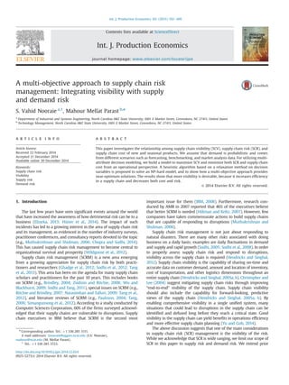
A multi-objective approach to supply chain risk
management: Integrating visibility with supply
and demand risk
S. Vahid Nooraie a,1
, Mahour Mellat Parast b,n
a
Department of Industrial and Systems Engineering, North Carolina A&T State University, 1601 E Market Street, Greensboro, NC 27411, United States
b
Technology Management, North Carolina A&T State University, 1601 E Market Street, Greensboro, NC 27411, United States
a r t i c l e i n f o
Article history:
Received 22 February 2014
Accepted 21 December 2014
Available online 30 December 2014
Keywords:
Supply chain risk
Visibility
Supply risk
Demand risk
a b s t r a c t
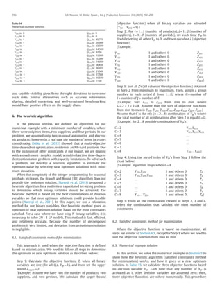
This paper investigates the relationship among supply chain visibility (SCV), supply chain risk (SCR), and
supply chain cost of new and seasonal products. We assume that demand is probabilistic and comes
from different scenarios such as forecasting, benchmarking, and market analysis data. For utilizing multi-
attribute decision modeling, we build a model to maximize SCV and minimize both SCR and supply chain
cost from an operational perspective. A heuristic algorithm based on a relaxation method on decision
variables is proposed to solve an NP-hard model, and to show how a multi-objective approach provides
near-optimum solutions. The results show that more visibility is desirable, because it increases efficiency
in a supply chain and decreases both cost and risk.
& 2014 Elsevier B.V. All rights reserved.
1. Introduction
The last few years have seen significant events around the world
that have increased the awareness of how detrimental risk can be to a
business (Elzarka, 2013; Hüner et al., 2014). The impact of such
incidents has led to a growing interest in the area of supply chain risk
and its management, as evidenced in the number of industry surveys,
practitioner conferences, and consultancy reports devoted to the topic
(e.g., Muthukrishnan and Shulman, 2006; Chopra and Sodhi, 2014).
This has caused supply chain risk management to become central to
organizational survival and prosperity (Wildgoose et al., 2012).
Supply chain risk management (SCRM) is a new area emerging
from a growing appreciation for supply chain risk by both practi-
tioners and researchers (Ghadge et al., 2012; Sodhi et al., 2012; Tang
et al., 2013). This area has been on the agenda for many supply chain
scholars and practitioners for the past 10 years. This includes books
on SCRM (e.g., Brindley, 2004; Zsidisin and Ritchie, 2008; Wu and
Blackhurst, 2009; Sodhi and Tang, 2011), special issues on SCRM (e.g.,
Ritchie and Brindley, 2007; Narasimhan and Talluri, 2009; Tang et al.,
2012), and literature reviews of SCRM (e.g., Paulsson, 2004; Tang,
2006; Simangunsong et al., 2012). According to a study conducted by
Computer Sciences Corporation, 60% of the firms surveyed acknowl-
edged that their supply chains are vulnerable to disruptions. Supply
chain executives in IBM believe that SCRM is the second most
important issue for them (IBM, 2008). Furthermore, research con-
ducted by AMR in 2007 reported that 46% of the executives believe
that better SCRM is needed (Hillman and Keltz, 2007). However, few
companies have taken commensurate actions to build supply chains
that are capable of responding to disruptions (Muthukrishnan and
Shulman, 2006).
Supply chain risk management is not just about responding to
natural disasters. There are many other risks associated with doing
business on a daily basis; examples are daily fluctuations in demand
and supply and rapid growth (Sodhi, 2005; Sodhi et al., 2008). In order
to properly assess supply chain risk and respond to disruptions,
visibility across the supply chain is required (Hendricks and Singhal,
2012). Supply chain visibility is the capability of sharing on-time and
accurate data on customer demand, amount and location of inventory,
cost of transportation, and other logistics dimensions throughout an
entire supply chain (Hendricks and Singhal, 2005a, b). Christopher and
Lee (2004) suggest mitigating supply chain risks through improving
“end-to-end” visibility of the supply chain. Supply chain visibility
should also include the capability for forward-looking, predictive
views of the supply chain (Hendricks and Singhal, 2005a, b). By
enabling comprehensive visibility in a single unified system, many
situations that could lead to disruptions in the supply chain can be
identified and defused long before they reach a critical state. Good
visibility in the supply chain can yield benefits in operations efficiency
and more effective supply chain planning (Yu and Goh, 2014).
The above discussion suggests that one of the main considerations
in supply chain risk (SCR) management is the visibility of the risk.
While we acknowledge that SCR is wide ranging, we limit our scope of
SCR in this paper to supply risk and demand risk. We extend prior
Contents lists available at ScienceDirect
journal homepage: www.elsevier.com/locate/ijpe
Int. J. Production Economics
http://dx.doi.org/10.1016/j.ijpe.2014.12.024
0925-5273/& 2014 Elsevier B.V. All rights reserved.
n
Corresponding author. Tel.: þ1 336 285 3111.
E-mail addresses: Snooraie@aggies.ncat.edu (S.V. Nooraie),
mahour@ncat.edu (M. Mellat Parast).
1
Tel.: þ1 336 285 3723.
Int. J. Production Economics 161 (2015) 192–200
studies in supply chain risk and supply chain visibility through using a
multi-objective approach to supply chain visibility and risk as recom-
mended by Yu and Goh (2014). In this approach, SCV has been
connected to the capability of obtaining up-to-date information on
demand, quantity and location of inventory, transport-connected cost,
and other logistics activities throughout an entire supply chain.
Similarly, SCR can be regarded as risks associated with incidents such
as an unanticipated event within a supply chain and the associated
negative outcomes of that event on the supply chain. There are
conflicting challenges between supply chain visibility and supply chain
risk. Our proposed model combines the objectives of SCV maximiza-
tion, SCR minimization, and supply chain cost minimization under the
constraints of budget, probabilistic customer demands, production
capacity, and supply availability assuming time parameter.
In this paper, we follow the recommendation and suggestion in
the literature provided by Yu and Goh (2014), considering a triple
objective of cost, risk, and visibility for the downstream supply
chain. We assume a condition that new time-dependent products
with demand under risk are included in the model. New seasonal
products (e.g., automotive, electronics) with demand under risk and
other time-dependent parameters increase the total complexity of
our model. Practically, our model is more applicable where we are
not sure about demand in each time period. In such a dynamic and
evolving market, we need to keep our supply chain visibility at a
high level while we face supply risk. This type of model can be used
for new products (e.g., automotive and electronic devices) where
products are newly developed and produced. New products have
such characteristics that when they arrive to the market for the first
time, they should maintain high visibility.
The remainder of this paper is organized as follows. First a
review of the literature on supply chain risk management and
supply chain visibility is provided. Then, the model is specified. In
order to examine how the model behaves, a numerical example
with limited variables is presented. Later, a heuristic algorithm is
developed to solve the numerical example with some analytical
discussion on results. Finally, we provide limitations and future
research directions.
2. Literature review
The study of supply chain visibility (SCV) has drawn considerable
interest from both researchers and practitioners in supply chain
management (Barlett, et al., 2007). In their analysis of supply chains,
Harland et al. (2003) report that half of the risk was visible to the focal
company. The central question in the relationship between supply
chain risk and supply chain visibility is how to choose suppliers in
order to minimize the supply risk and how to enhance visibility
without exceeding the production or total budgets. According to
Enslow (2006), about 79% of the large companies surveyed globally
cited lack of SCV as their top concern. Furthermore, an alarming 90%
of the responding supply chains asserted that their existing supply
chain technology is incapable of providing timely information to
prepare budget and cash flow plans for the finance department.
Delen et al. (2007) and Zhou (2009) argue that through the
implementation of RFID, SCV can be enhanced to eliminate supply
chain barriers by enabling and sharing information and eventually
improving supply chain performance. Ouyang (2007) further shows
that SCV implementation can enhance supply chain stability and
mitigate the bullwhip effect. This concurs with Goh et al. (2009), who
define SCV as the capability of a supply chain actor to access to or to
provide the required timely information/knowledge in the supply
chain from/to relevant supply chain partners for better decisions.
While some work on visibility in supply chains has been under-
taken, this area is still nascent (e.g., Smaros et al., 2003). Zhang et al.
(2010) have also reported that global supply chain and logistics
operators clearly seemed to benefit from end-to-end visibility of the
supply chain. Thus, there is a need to better understand and properly
examine the overall impact of supply chain visibility, supply chain risk,
and supply chain cost in the context of multiple objectives. In a review
of the current status of research and scholarly work in supply chain
risk management, Sodhi et al. (2012) refer to the methodological gap
in this area. Our study addresses this issue from the methodological
aspect, while providing insight for practitioners on how to address
risk, visibility, and cost in the context of a supply chain.
This study extends prior research in supply chain risk and supply
chain visibility in several ways. We define demand as a probabilistic
parameter that comes from known scenarios (Lau et al., 2000).
Moreover, we define risk in based on any type of supplier risk. Each
supplier imposes risk on our model, and we need to minimize total
risk from the supply side. We consider specifically the context of a
focal firm that has to strategically consider the triple objectives of
cost, risk, and visibility for the downstream supply chain (push
strategy), while demand is probabilistic for new products along with
the complexity that comes from the time-dependent parameter.
3. Model development
A mathematical model is developed incorporating SCV and SCR
as well as supply chain cost, so that the appropriate suppliers can be
identified. The proposed multiple-objective integer programming
model includes three objectives: visibility maximization, risk mini-
mization, and cost minimization. The formulation of the model is
described as follows.
Index variables
i index of products
j index of suppliers
t index of time
Decision variables
Qijt quantity of product i provided by supplier j in period t
Yijt a binary variable determined by whether product i is
supplied by supplier j in period t
Parameters
Bit budget available to enhance SCV for product i in period t
Cjt production capacity of supplier j in period t
CRijt cost of reducing supply risk for product i from supplier j
in period t
CVijt cost of enhancing SCV to current level for product i from
supplier j in period t
Dit demand of product i in period t
mijt minimum order quantity for product i required by
supplier j in period t
Pijt purchase price for product i supplied by supplier j in
period t
IRijt impact (financial loss) caused by supply risk for product i
from supplier j in period t
Rijt supply risk for product i from supplier j in period t
Rit maximum allowable supply risk for product i in period t
Vijt supply chain visibility incurred if product i is supplied by
supplier j in period t
Vit minimum amount of visibility needed for product i in
period t
Model:
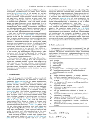
Max visibility ¼
X
i
X
j
X
t
VijtYijt ð1Þ
Min Risk ¼
X
i
X
j
X
t
RijtYijt ð2Þ
S.V. Nooraie, M. Mellat Parast / Int. J. Production Economics 161 (2015) 192–200 193
Min Cost ¼
P
i
P
j
P
tVijtCVijtYijt þ
P
i
P
j
P
tRijtCRijtYijt
þ
X
i
X
j
X
t
IRijtYijt þ
X
i
X
j
X
t
PijtQijt ð3Þ
Subject to:
X
j
VijtCVijtYijt rBitfor each i; t ð4Þ
X
j
VijtYijt ZVitfor each i; t ð5Þ
X
j
Qijt ZDn
it ð6Þ
Dn
it is the expected value of demand which is equal Dit (demand
of product i in period t  P (corresponding probability))
X
i
Qijt rCjtYijtfor each j; t ð7Þ
X
j
RijtYijt rRitfor each i; t ð8Þ
Qijt ZmijtYijtfor each i; j; t ð9Þ
Qijt rNYijtfor each i ð10Þ
Qijt Z0 for each i; j; t ð11Þ
Yijt is 0; 1 for each i; j; t ð12Þ
Constraint (4) restricts the spending of SCV under a planned
budget for all suppliers. Constraint (5) examines the minimum
amount of visibility for each product. Constraint (6) sets probabilistic
demand (discrete probability) quantity for each product where
probability is discrete. Constraint (7) serves as the capacity con-
straint for each supplier. Constraint (8) limits the maximum allow-
able supply risk for each product supplied by all suppliers.
Constraint (9) specifies the minimum order quantity of each product
for all suppliers. Constraint (10) prevents a conflict of the decision
variables, where N is a relatively large number (it is necessary to
assign a large number). Constraint (11), while redundant, preserves
the non-negativity of each amount of each product. Constraint (12)
is the definition of a binary variable.
4. Demand risk calculations
In this section, we discuss demand under risk as well as the
origin of risk. As mentioned earlier, we assume demand comes from
different scenarios with different probabilities. That means if the
sum of all probabilities equals one, the summation of all scenarios'
probabilities in association with demand should equal one. In the
real case for our model, the possible scenarios are defined as
forecasting, benchmarking, and market analysis data. Each scenario
has its characteristics and provides us an approximation of future
demand. In this case, we define Pi as the probability of the ith
scenario with the quantity of demand.
To solve the mathematical problem, we propose the follow-
ing method: If pi (i¼1…n) is the probability of each demand as
P
pi (i¼ 1…n)¼1, where Dm (m¼ 1…n) denotes n scenarios for demand
with probability pi. To simplify calculation in the model, we calculate
the expected value for each i,m for each scenario by
P
Pi  Dm for
each i,m.
5. Numerical example
The main purpose of this numerical example is to show how
the model works. Assume a problem where we have two products
from the same two suppliers, four independent periods (four
seasons), and we need to maximize visibility and minimize risk
and cost in our mathematical model. The values of our index
variables are i (index of products)¼1 or 2, j (index of suppliers)¼1
or 2, and t (index of time)¼1–4. The following tables give amounts
of each model parameter.
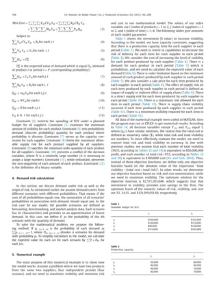
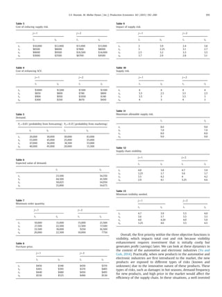
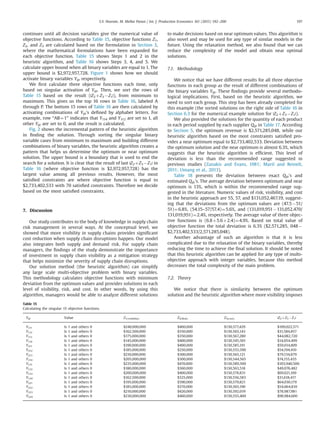
Table 1 shows the investment ($ value) to increase visibility.
According to the model, we have capacity constraint, suggesting
that there is a production capacity limit for each supplier in each
period (Table 2). We need to invest in capabilities to decrease the
risk of delivery for each item for each supplier in each period
(Table 3). We consider the cost of increasing the level of visibility
for each product produced by each supplier (Table 4). There is a
demand for each product in each period (Table 5) which is
probabilistic, and we need to calculate the expected value of each
demand (Table 6). There is order limitation based on the minimum
amount of each product produced by each supplier in each period
(Table 7). We also consider a sale price for each item produced by
each supplier in each period (Table 8). The effect of supply risk on
each item produced by each supplier in each period is defined as
impact of supply or indirect effect of supply chain (Table 9). There
is a direct supply risk for each item produced by each supplier in
each period (Table 10). There is a maximum risk allowed for each
item in each period (Table 11). There is supply chain visibility
occurred if each item produced by each supplier in each period
(Table 12). There is a minimum visibility required for each item in
each period (Table 13).
All data of the numerical example were coded in MATLAB; then
the program was run in CPLEX to get numerical results. According
to Table 14, all decision variables except Y111 and Y112 equal 1,
where Qijt's have similar solutions. We realize that the total cost is
defined as monetary value ($), while total risk and total visibility
are numbers. To more effectively evaluate the model, we need to
convert total risk and total visibility to currency. In line with
previous studies, we assume that each number of total visibility
(54.15, according to Tables 12 and 14) is equivalent to $50,000,000
profit, and each number of total risk (47.5, according to Tables 14
and 10) is equivalent to $100,000 cost (Yu and Goh, 2014). Thus,
instead of three objective functions, we define only one objective
function based on the absolute value of the expression “total
visibilityÀ(total costþtotal risk)”. In other words, we determine
our objective function based on risk and cost minimization, while
we need to maximize visibility. The optimum solution for the
objective function is $2,571,285,048, which suggests that that
investment in visibility provides cost savings to the firm. The
optimum levels of the numeric values of risk, visibility, and cost
are 52, 54.15, and $131,019,951.69, respectively.
Table 1
Available budget for SCV.
i1 i2
t1 $100,000 $135,000
t2 $120,000 $115,000
t3 $90,000 $110,000
t4 $115,000 $145,000
Table 2
Production capacity.
j1 j2
t1 50,000 80,000
t2 80,000 80,000
t3 90,000 70,000
t4 60,000 70,000
S.V. Nooraie, M. Mellat Parast / Int. J. Production Economics 161 (2015) 192–200194
Overall, the first priority within the three objective functions is
visibility, which impacts total cost and risk because visibility
enhancement requires investment that is initially costly but
generates profit (savings) later. We can look at these dynamics in
the context of the automotive and electronic industries (Yu and
Goh, 2014). Practically, when new products in the automotive and
electronic industries are first introduced to the market, the new
products are exposed to different types of risks (known and
unknown) due to the innovative nature of these products. These
types of risks, such as damages in hot seasons, demand frequency
for new products, and high price in the market would affect the
efficiency of the supply chain. In these situations, a well invested
Table 3
Cost of reducing supply risk.
j¼1 j¼2
i1 i2 i1 i2
t1 $10,000 $12,000 $11,000 $11,000
t2 $8500 $8000 $7800 $8000
t3 $9000 $9500 $10,500 $14,000
t4 $3000 $3500 $6700 $4500
Table 4
Cost of enhancing SCV.
j¼1 j¼2
i1 i2 i1 i2
t1 $1000 $1200 $1100 $1100
t2 $850 $800 $780 $800
t3 $900 $950 $1050 $140
t4 $300 $350 $670 $450
Table 5
Demand.
P1¼0.65 (probability from forecasting) P2¼0.35 (probability from marketing)
i1 i2 i1 i2
t1 20,000 30,000 30,000 43,000
t2 55,000 45,000 25,000 35,000
t3 67,000 36,000 18,500 33,000
t4 40,000 45,000 20,000 15,500
Table 6
Expected value of demand.
i1 i2
t1 23,500 34,550
t2 44,500 41,500
t3 50,025 34,950
t4 33,000 34,675
Table 7
Minimum order quantity.
j¼1 j¼2
i1 i2 i1 i2
t1 10,000 15,000 15,000 21,500
t2 27,500 22,500 12,500 17,500
t3 33,500 18,000 9250 16,500
t4 20,000 22,500 10,000 7750
Table 8
Purchase price.
j¼1 j¼2
i1 i2 i1 i2
t1 $450 $340 $430 $370
t2 $365 $395 $370 $405
t3 $440 $480 $450 $495
t4 $530 $525 $490 $530
Table 9
Impact of supply risk.
j¼1 j¼2
i1 i2 i1 i2
t1 2 3.9 2.4 3.8
t2 3 2.25 3.1 2.7
t3 2.5 3.2 3.3 3.5
t4 3.7 2.9 2.8 3.1
Table 10
Supply risk.
j¼1 j¼2
i1 i2 i1 i2
t1 4 4 4 4
t2 3.5 2.5 3.5 2.5
t3 3.5 3 3.5 3
t4 4 3 4 3
Table 11
Maximum allowable supply risk.
i1 i2
t1 8.0 9.0
t2 7.0 7.0
t3 8.0 8.0
t4 9.0 9.0
Table 12
Supply chain visibility.
j¼1 j¼2
i1 i2 i1 i2
t1 4.8 3.8 4.7 3.9
t2 3.25 3.7 3.6 3.7
t3 3.5 4.2 4 4.2
t4 2.9 4.1 3.25 4.6
Table 13
Minimum visibility needed.
j¼1 j¼2
i1 i2 i1 i2
t1 4.7 3.9 5.5 4.0
t2 3.6 3.7 3.5 3.5
t3 4.0 4.20 4.0 5.0
t4 3.25 4.6 3.5 4.5
S.V. Nooraie, M. Mellat Parast / Int. J. Production Economics 161 (2015) 192–200 195
and capable visibility gives firms the right directions to overcome
such risks. Similar alternatives such as accurate information
sharing, detailed marketing, and well-structured benchmarking
would have positive effects on the supply chain.
6. The heuristic algorithm
In the previous section, we defined an algorithm for our
numerical example with a minimum number of variables, where
there were only two items, two suppliers, and four periods. In our
problem, we assumed only two seasonal automotive and electro-
nic products; however in a real case the number of items increases
considerably. Dabia et al. (2013) showed that a multi-objective
time-dependent optimization problem is an NP-hard problem. Due
to the inclusion of other constraints in our model, we are dealing
with a much more complex model, a multi-objective time-depen-
dent optimization problem with capacity limitations. To solve such
a problem, we develop a heuristic algorithm to estimate the
optimum value by selecting near optimum solutions with mini-
mum deviation.
When the complexity of the integer programming for seasonal
products increases, the Branch and Bound (BB) algorithm does not
provide the optimum solution. Narenji et al. (2011) proposed a
heuristic algorithm for a multi-item capacitated lot-sizing problem
to determine which binary variables should be activated. The
heuristic method is based on the best combinations of decision
variables so that near optimum solutions could provide feasible
points (Narenji et al., 2011). In this paper, we use a relaxation
method for our binary variables. Our heuristic method gives an
optimum or near optimum solution based on the most constraints
satisfied. For a case where we have only N binary variables, it is
necessary to solve 2NÀ1 LP models. This method is fast, efficient,
and relatively accurate, because the number of decomposed
problems is very limited, and deviation from an optimum solution
is negligible.
6.1. Satisfied constraints method for minimization
This approach is used when the objective function is defined
based on minimization. We need to follow all steps to determine
the optimum or near optimum solution as described below:
Step 1: Calculate the objective function, Z, when all binary
variables are one (for all i,j,t, Yijt ¼1), and then set the upper
bound Zupper ¼Z.
(Example: Assume we have two the number of products, two
suppliers, and two periods. We calculate the upper bound
(objective function) when all binary variables are activated
(Y111…Y222 ¼1).)
Step 2: For i¼1…I (number of products), j¼1…J (number of
suppliers), t¼1…T (number of periods), set each time Yijt to
1 while setting all other Yijt to 0, and then calculate Z (objective
function).
(Example:
Y111 1 and others 0 Z111
Y121 1 and others 0 Z121
Y112 1 and others 0 Z112
Y211 1 and others 0 Z211
Y212 1 and others 0 Z212
Y122 1 and others 0 Z122
Y221 1 and others 0 Z221
Y222 1 and others 0 Z222)
Step 3: Sort all Z's (all values of the objective function) obtained
in Step 2 from minimum to maximum. Then, assign a group
number to each sorted Z from 1…G, where G¼number of
I Â number of J Â number of T.
(Example: Sort Z111 to Z222 from min to max where
G¼2 Â 2 Â 2¼8. Assume that the sort of objective functions
from min to max is Z111, Z121, Z112, Z211, Z212, Z122, Z221, Z222.)
Assume that C is the nth (n¼2…8) combination of Yijt's where
the total number of all combinations after Step 2 is equal C¼G.
(Example: for 2…8 possible combination of Yijt's
C¼2 Y111,Y121
C¼3 Y111,Y121,Y112
C¼4 …
C¼5 …
C¼6 …
C¼7 …
C¼8 Y111…Y222)
Step 4: Using the sorted order of Yijt's from Step 3 follow the
chart below:
(Example: algorithm stops when C¼8
C¼2 Y111,Y121 1 and others 0 Z2
C¼3 Y111,Y121,Y112 1 and others 0 Z3
C¼4 … 1 and others 0 Z4
C¼5 … 1 and others 0 Z5
C¼6 … 1 and others 0 Z6
C¼7 … 1 and others 0 Z7
C¼8 Y111…Y222 1 and others 0 Z8)
Step 5: From all the combination created in Steps 2, 3 and 4,
select the combination that satisfies the most number of
constraints.
6.2. Satisfied constraints method for maximization
When the objective function is based on maximization, all
steps are similar to Section 6.1, except for Step 3 where we need to
sort the objective function from max to min.
6.3. Numerical example solution
In this section, we solve the numerical example in Section 5 to
show how the heuristic algorithm (satisfied constraints method
for minimization) works, and how it gives us a near optimum
solution. In Table 15, we calculate three objective functions based
on decision variable Yijt. Each time that any number of Yijt is
activated as 1, other decision variables are assumed zero; then,
three objective functions are solved numerically. This procedure
Table 14
Numerical example solution.
Y111 is: 0 Q111 is: 0
Y112 is: 0 Q112 is: 0
Y113 is: 1 Q113 is: 40,775
Y114 is: 1 Q114 is: 20,000
Y121 is: 1 Q121 is: 23,500
Y122 is: 1 Q122 is: 44,500
Y123 is: 1 Q123 is: 9250
Y124 is: 1 Q124 is: 13,000
Y211 is: 1 Q211 is: 15,000
Y212 is: 1 Q212 is: 24,000
Y213 is: 1 Q213 is: 18,450
Y214 is: 1 Q214 is: 26,925
Y221 is: 1 Q221 is: 21,500
Y222 is: 1 Q222 is: 17,500
Y223 is: 1 Q223 is: 16,500
Y224 is: 1 Q224 is: 7750
S.V. Nooraie, M. Mellat Parast / Int. J. Production Economics 161 (2015) 192–200196
continues until all decision variables give the numerical value of
objective functions. According to Table 15, objective functions Z1,
Z2, and Z3 are calculated based on the formulation in Section 3,
where the mathematical formulations have been expanded for
each objective function. Table 15 shows Steps 1 and 2 in the
heuristic algorithm, and Table 16 shows Steps 3, 4, and 5. We
calculate upper bound when all binary variables are equal to 1. The
upper bound is $2,972,957,728. Figure 1 shows how we should
activate binary variables Yijt respectively.
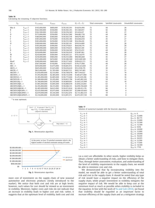
We first calculate three objective functions each time, only
based on singular activation of Yijt. Then, we sort the rows of
Table 15 based on the result (|Z2 þZ3 ÀZ1|), from minimum to
maximum. This gives us the top 16 rows in Table 16, labeled A
through P. The bottom 15 rows of Table 16 are then calculated by
activating combinations of Yijt's defined by alphabet letters. For
example, row “AB¼1” indicates that Y114 and Y112 are set to 1, all
other Yijt are set to 0, and the result is calculated.
Fig. 2 shows the incremental pattern of the heuristic algorithm
in finding the solution. Through sorting the singular binary
variable cases from minimum to maximum and building different
combinations of binary variables, the heuristic algorithm creates a
pattern that helps us determine the optimum or near optimum
solution. The upper bound is a boundary that is used to end the
search for a solution. It is clear that the result of last |Z2 þZ3 ÀZ1| in
Table 16 (where objective function is $2,972,957,728) has the
largest value among all previous results. However, the most
satisfied constraints are where objective function is equal to
$2,733,402,533 with 70 satisfied constraints. Therefore we decide
based on the most satisfied constraints.
7. Discussion
Our study contributes to the body of knowledge in supply chain
risk management in several ways. At the conceptual level, we
showed that more visibility in supply chains provides significant
cost reduction when supply chain disruptions happen. Our model
also integrates both supply and demand risk. For supply chain
managers, the findings of the study demonstrate the importance
of investment in supply chain visibility as a mitigation strategy
that helps minimize the severity of supply chain disruptions.
Our solution method (the heuristic algorithm) can simplify
any large scale multi-objective problem with binary variables.
This methodology calculates objective functions with minimum
deviation from the optimum values and provides solutions in each
level of visibility, risk, and cost. In other words, by using this
algorithm, managers would be able to analyze different solutions
to make decisions based on near optimum values. This algorithm is
also novel and may be used for any type of similar models in the
future. Using the relaxation method, we also found that we can
reduce the complexity of the model and obtain near optimal
solutions.
7.1. Methodology
We notice that we have different results for all three objective
functions in each group as the result of different combinations of
the binary variables Yijt. These findings provide several methodo-
logical implications. First, based on the heuristic algorithm, we
need to sort each group. This step has been already completed for
this example (the sorted solutions on the right side of Table 16 in
Section 6.3 for the numerical example solution for |Z2 þZ3 ÀZ1|).
We also provided the solutions for the quantity of each product
in each period supplied by each supplier Qijt in Table 17. According
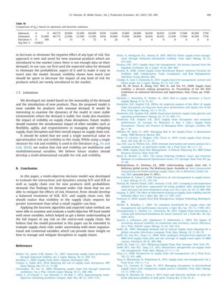
to Section 5, the optimum revenue is $2,571,285,048, while our
heuristic algorithm based on the most constraints satisfied pro-
vides a near optimum equal to $2,733,402,533. Deviation between
the optimum solution and the near optimum is almost 6.3%, which
suggests that the heuristic algorithm is efficient. This level of
deviation is less than the recommended range suggested in
previous studies (Zanakis and Evans, 1981; Martí and Reinelt,
2011; Umang et al., 2013).
Table 18 presents the deviation between exact Qijt's and
estimated Qijt's. The average deviation between optimum and near
optimum is 13%, which is within the recommended range sug-
gested in the literature. Numeric values of risk, visibility, and cost
in the heuristic approach are 55, 57, and $131,052,467.19, suggest-
ing that the deviations from the optimum values are (47.5À51/
51)¼6.8%, (54.15–57/57.4)¼5.6%, and (131,019,951À131,052,470/
131,019,951)¼2.4%, respectively. The average value of three objec-
tive functions is (6.8þ5.6þ2.4)¼4.9%. Based on total value of
objective function the total deviation is 6.3% ($2,571,285, 048À
$2,733,402,533/2,571,285,048).
Another advantage of such an algorithm is that it is less
complicated due to the relaxation of the binary variables, thereby
reducing the time to achieve the final solution. It should be noted
that this heuristic algorithm can be applied for any type of multi-
objective approach with integer variables, because this method
decreases the total complexity of the main problem.
7.2. Theory
We notice that there is similarity between the optimum
solution and the heuristic algorithm where more visibility imposes
Table 15
Calculating the singular 15 objective functions.
Yijt Value Z1(visibility) Z2(Risk) Z3(cost) |Z2þZ3 ÀZ1|
Y111 Is 1 and others 0 $240,000,000 $400,000 $130,577,429 $109,022,571
Y112 Is 1 and others 0 $162,500,000 $350,000 $130,565,143 $31,584,857
Y113 Is 1 and others 0 $175,000,000 $350,000 $130,567,280 $44,082,720
Y114 Is 1 and others 0 $145,000,000 $400,000 $130,545,501 $14,054,499
Y211 Is 1 and others 0 $190,000,000 $400,000 $130,585,191 $59,014,809
Y212 Is 1 and others 0 $185,000,000 $250,000 $130,555,590 $54,194,410
Y213 Is 1 and others 0 $210,000,000 $300,000 $130,565,121 $79,134,879
Y214 Is 1 and others 0 $205,000,000 $300,000 $130,544,565 $74,155,435
Y121 Is 1 and others 0 $235,000,000 $470,000 $130,589,500 $103,940,500
Y122 Is 1 and others 0 $180,000,000 $360,000 $130,563,518 $49,076,482
Y123 Is 1 and others 0 $200,000,000 $400,000 $130,578,831 $69,021,169
Y124 Is 1 and others 0 $162,500,000 $325,000 $130,556,583 $31,618,417
Y221 Is 1 and others 0 $195,000,000 $390,000 $130,579,821 $64,030,179
Y222 Is 1 and others 0 $185,000,000 $370,000 $130,565,190 $54,064,810
Y223 Is 1 and others 0 $210,000,000 $420,000 $130,592,019 $78,987,981
Y224 Is 1 and others 0 $230,000,000 $460,000 $130,555,400 $98,984,600
S.V. Nooraie, M. Mellat Parast / Int. J. Production Economics 161 (2015) 192–200 197
more cost of investment on the supply chain of new seasonal
automotive and electronic products (newly introduced to the
market). We notice that both cost and risk are at high levels;
however, such values for cost should be viewed as an investment
in visibility. Moreover, higher costs and risks do not indicate that
an increase in visibility leads to higher cost and risk; rather, it
suggests that at the optimum level of visibility, both cost and risk
(as a cost) are affordable. In other words, higher visibility helps us
obtain a better understanding of risks, and how to mitigate them.
Thus, through better assessment, evaluation, and understanding of
the level of visibility requirements in the supply chain, we would
be able to minimize cost and risk.
We demonstrated that by incorporating visibility into the
model, we would be able to get a better understanding of total
risk and cost in the supply chain. It should be noted that any type
of risk would have a negative impact on the efficiency of the
supply chain, while proper investment in visibility mitigates the
negative impact of risk. We would be able to keep cost at the
minimum level as much as possible when visibility is included in
the equation. In line with the work of Yu and Goh (2014), we found
that visibility should be regarded as an important factor to
increase efficiency of the supply chain and as a mitigation strategy
Table 16
Calculating the remaining 15 objective functions.
Yijt Z1(visibility) Z2(Risk) Z3(cost) |Z2þZ3 ÀZ1| Total constraints Satisfied constraints Unsatisfied constraints
Min A Y114¼1 $145,000,000 $400,000 $130,545,501 $14,054,499 72 44 28
B Y112¼1 $162,500,000 $350,000 $130,565,143 $31,584,857 72 42 30
C Y124¼1 $162,500,000 $325,000 $130,556,583 $31,618,417 72 45 27
D Y113¼1 $175,000,000 $350,000 $130,567,280 $44,082,720 72 44 28
E Y122¼1 $180,000,000 $360,000 $130,563,518 $49,076,482 72 45 27
F Y222 ¼1 $185,000,000 $370,000 $130,565,190 $54,064,810 72 45 27
G Y212 ¼1 $185,000,000 $250,000 $130,555,590 $54,194,410 72 45 27
H Y211¼1 $190,000,000 $400,000 $130,585,191 $59,014,809 72 44 28
I Y221¼1 $195,000,000 $390,000 $130,579,821 $64,030,179 72 44 28
J Y123¼1 $200,000,000 $400,000 $130,578,831 $69,021,169 72 45 27
K Y214 ¼1 $205,000,000 $300,000 $130,544,565 $74,155,435 72 44 28
L Y223 ¼1 $210,000,000 $420,000 $130,592,019 $78,987,981 72 44 28
M Y213 ¼1 $210,000,000 $300,000 $130,565,121 $79,134,879 72 44 28
N Y224¼1 $230,000,000 $460,000 $130,555,400 $98,984,600 72 45 27
O Y121 ¼1 $235,000,000 $470,000 $130,589,500 $103,940,500 72 45 27
MaxP Y111 ¼1 $240,000,000 $400,000 $130,577,429 $109,022,571 72 43 29
AB¼1 $307,500,000 $750,000 $130,578,017 $176,171,983 72 44 28
ABC¼1 $470,000,000 $1,075,000 $130,601,972 $338,323,028 72 47 25
ABCD¼1 $645,000,000 $1,425,000 $130,636,624 $512,938,376 72 49 23
ABCDE¼1 $825,000,000 $1,785,000 $130,667,515 $692,547,485 72 51 21
ABCDEF¼1 $1,010,000,000 $2,155,000 $130,700,078 $877,144,922 72 53 19
ABCDEFG¼1 $1,195,000,000 $2,405,000 $130,723,040 $1,061,871,960 72 54 18
ABCDEFGH¼1 $1,385,000,000 $2,805,000 $130,775,604 $1,251,419,396 72 56 16
ABCDEFGHI¼1 $1,580,000,000 $3,195,000 $130,822,798 $1,445,982,202 72 59 13
ABCDEFGHIJ¼1 $1,780,000,000 $3,595,000 $130,869,001 $1,645,535,999 72 62 10
ABCDEFGHIJK¼1 $1,985,000,000 $3,895,000 $130,880,939 $1,850,224,061 72 63 9
ABCDEFGHIJKL¼1 $2,195,000,000 $4,315,000 $130,940,331 $2,059,744,669 72 64 8
ABCDEFGHIJKLM¼1 $2,405,000,000 $4,615,000 $130,972,824 $2,269,412,176 72 66 6
ABCDEFGHIJKLMN¼1 $2,635,000,000 $5,075,000 $130,995,597 $2,498,929,403 72 68 4
ABCDEFGHIJKLMNO¼1 $2,870,000,000 $5,545,000 $131,052,470 $2,733,402,533 72 70*
2
ABCDEFGHIJKLMNOP¼1 $3,110,000,000 $5,945,000 $131,097,272 $2,972,957,728 72 68 4
n
Is near optimum.
For C = 2…G activate C first Yijt’s in
step 3 (Yijt =1), then calculate Zc
(objective function)
Zc < = upper
bound?
Yes No
C = C +1
Stop when C = G
Fig. 1. Minimization algorithm.
$0
$500,000,000
$1,000,000,000
$1,500,000,000
$2,000,000,000
$2,500,000,000
$3,000,000,000
$3,500,000,000
1 3 5 7 9 11 13 15 17 19 21 23 25 27 29 31
|Z2+Z3-Z1|
upperbound
At this point, we have 70 satisfied constraints which is the
highest number of satisfied constraints among all results.
Fig. 2. Minimization algorithm.
Table 17
Solution of numerical example with the heuristic algorithm.
Y111 is: 0 Q111 is: 0
Y112 is: 1 Q112 is: 32,000
Y113 is: 1 Q113 is: 40,775
Y114 is: 1 Q114 is: 23,000
Y121 is: 1 Q121 is: 23,500
Y122 is: 1 Q122 is: 12,500
Y123 is: 1 Q123 is: 9250
Y124 is: 1 Q124 is: 10,000
Y211 is: 1 Q211 is: 15,000
Y212 is: 1 Q212 is: 24,000
Y213 is: 1 Q213 is: 18,450
Y214 is: 1 Q214 is: 26,925
Y221 is: 1 Q221 is: 21,500
Y222 is: 1 Q222 is: 17,500
Y223 is: 1 Q223 is: 16,500
Y224 is: 1 Q224 is: 7750
S.V. Nooraie, M. Mellat Parast / Int. J. Production Economics 161 (2015) 192–200198
to decrease or eliminate the negative effect of any type of risk. Our
approach is new and novel for new seasonal products which are
introduced to the market (since there is not enough data on their
demand). In our case, we first used the expected value for demand
to eliminate the probabilistic aspect of it and to make it easy to
insert into the model. Second, visibility shows how much cost
should be spent to decrease the impact of any kind of risk for
products which are newly introduced to the market.
7.3. Limitations
We developed our model based on the seasonality of the demand
and the introduction of new products. Thus, the proposed model is
most suitable for products with seasonal demand. It would be
interesting to examine the dynamics of the model in more stable
environments where the demand is stable. Our study also examines
the impact of visibility on supply chain disruptions. Future studies
should examine the simultaneous impact of other variables such as
flexibility, agility, and responsiveness in managing and mitigating
supply chain disruption and their overall impact on supply chain cost.
It should be noted that we used a single numerical value to
operationalize risk and visibility in this study. While using a single
measure for risk and visibility is used in the literature (e.g., Yu and
Goh, 2014), we realize that risk and visibility are multifactor and
multidimensional variables. We believe future studies should
develop a multi-dimensional variable for risk and visibility.
8. Conclusion
In this paper, a multi-objective decision model was developed
to evaluate the interactions and dynamics among SCV and SCR as
well as supply chain cost for new products with probabilistic
demand. Our findings for demand under risk show that we are
able to mitigate the effects of risk. However, firms should develop
a balanced treatment of SCR, SCV, and supply chain cost. We
should realize that visibility in the supply chain requires far
greater investment than what a small supplier can bear.
Applying the heuristic algorithm and expected value method, we
were able to examine and evaluate a multi-objective NP-hard model
with more variables, which helped us get a better understanding of
the full impact of any risk on the end-to-end supply chain. We
believe that the model presented in this paper can be extended to
evaluate supply chain risks under uncertainty with more organiza-
tional and contextual variables, which can provide more insight on
how to manage and mitigate disruptions in supply chains.
References
Barlett, P.A., Julien, D.M., Baines, T.S., 2007. Improving supply chain performance
through improved visibility. Int. J. Logist. Manag. 18 (2), 294–313.
Brindley, C., 2004. Supply Chain Risks. Ashgate, Burlington, MA.
Chopra, S., Sodhi, M.S., 2014. Reducing the risk of supply chain disruptions. MIT
Sloan Manag. Rev. 55 (3), 73–80.
Christopher, M., Lee, H., 2004. Mitigating supply chain risk through improved
confidence. Int. J. Phys. Distrib. Logist. Manag. 34 (5), 388–396.
Dabia, S., El-Ghazali, T., van Woensel, T., De Kok, T., 2013. Approximating multi-
objective scheduling problems. Comput. Oper. Res. 40 (5), 1165–1175.
Delen, D., Hardgrave, B.C., Sharda, R., 2007. RFID for better supply-chain manage-
ment through enhanced information visibility. Prod. Oper. Manag. 16 (5),
613–624.
Elzarka, S.M., 2013. Supply chain risk management: the lessons learned from the
Egyptian revolution. Int. J. Logist. 16 (6), 482–492.
Enslow, B., 2006. Global Supply Chain Benchmark Report: Industry Priorities for
Visibility: B2B, Collaboration, Trade, Compliance, and Risk Management.
Aberdeen Group, Boston, MA.
Ghadge, A., Dani, S., Kalawsky, R., 2012. Supply chain risk management: present and
future scope. Int. J. Logist. Manag. 23 (3), 313–339.
Goh, M., De Souza, R., Zhang, A.N., Wei, H., and Tan, P.S. (2009. Supply chain
visibility: a decision making perspective. In: Proceedings of the 4th IEEE
Conference on Industrial Electronics and Applications, Xian, China, pp. 2546–
2551.
Harland, C., Brenchley, R., Walker, H., 2003. Risk in supply networks. J. Purch.
Supply Manag. 9 (2), 51–62.
Hendricks, K.B., Singhal, V.R., 2005a. An empirical analysis of the effect of supply
chain disruptions on long-run stock price performance and equity risk of the
firm. Prod. Oper. Manag. 14 (1), 35–52.
Hendricks, K.B., Singhal, V.R., 2005b. Association between supply chain glitches and
operating performance. Manag. Sci. 51 (5), 695–711.
Hendricks, K.B., Singhal, V.R., 2012. Supply chain disruptions and corporate
performance. In: Gurnani, H., Mehrotra, A., Ray, S. (Eds.), Supply Chain
Disruptions: Theory and Practice of Managing Risks. Springer, London, UK,
pp. 1–19.
Hillman, M., Keltz, H., 2007. Managing Risk in the Supply Chain: A Quantitative
Study. AMR Research, Boston, MA.
Hüner, D., Larsoon, T., Wagner, S.M., Christ, A., 2014. Costly supply chain disrup-
tions. Ind. Eng. 46 (3), 32–37.
Lau, A.H., Lau, H., Willett, K.D., 2000. Demand uncertainty and returns policies for a
seasonal product: an alternative model. Int. J. Prod. Econ. 66 (1), 1–12.
IBM, 2008. Supply Chain Risk Management: A Delicate Balancing Act. IBM Global
Business Services, New York, NY.
Martí, R., Reinelt, G., 2011. The Linear Ordering Problem: Exact and Heuristic
Methods in Combinatorial Optimization Series. 175. Springer, New York, NY, pp.
17–40.
Muthukrishnan, R., Shulman, J.A., 2006. Understanding supply chain risk: A
McKinsey global survey. The McKinsey Quart. Available at: http://www.mckin
seyquarterly.com/Understanding_supply_chain_risk_A_McKinsey_Global_Sur
vey_1847 (accessed June 11, 2011).
Narasimhan, R., Talluri, S., 2009. Perspectives on risk management in supply chains.
J. Oper. Manag. 27 (2), 114–118.
Narenji, M., Fatemi Ghomi, S.M.T., Nooraie, S.V.R., 2011. Grouping in decomposition
method for multi-item capacitated lot-sizing problem with immediate lost
sales and joint and item-dependent setup cost. Int. J. Syst. Sci. 42 (3), 489–498.
Ouyang, Y., 2007. The effect of information sharing on supply chain stability and the
bullwhip effect. Eur. J. Oper. Res. 182 (3), 1107–1121.
Paulsson, U., 2004. Supply Chain Risk Management. Ashgate Publishing, Burlington,
MA.
Ritchie, B., Brindley, C., 2007. An emergent framework for supply chain risk
management and performance measures. J. Oper. Res. Soc. 58 (11), 1398–1411.
Simangunsong, E., Hendry, L.C., Stevenson, M., 2012. Supply-chain uncertainty: a
review and theoretical foundation for future research. Int. J. Prod. Res. 50 (16),
4493–4523.
Smaros, J., Lehtonen, J.M., Appelqvist, P., Holmstrom, J., 2003. The impact of
increasing demand visibility on production and inventory control efficiency.
Int. J. Phys. Distrib. Logist. Manag. 33 (4), 336–354.
Sodhi, M., 2005. Managing demand risk in tactical supply chain planning for a
global consumer electronics company. Prod. Oper. Manag. 14 (1), 69–79.
Sodhi, M., Son, B.G., Tang, C.S., 2008. What employers demand from applicant for
MBA-level supply chain jobs and the coverage of supply chain topics in MBA
courses. Interfaces 38 (6), 469–484.
Sodhi, M., Tang, C.S., 2011. Mitigating Supply Chain Risk. Springer, New York, NY.
Sodhi, M.S., Son, B.G., Tang, C.S., 2012. Researchers' perspectives on supply chain
risk management. Prod. Oper. Manag. 21 (1), 1–13.
Tang, C.S., 2006. Perspectives in supply chain risk management. Int. J. Prod. Econ.
103 (2), 451–488.
Tang, O., Matsukawa, H., Nakashima, K., 2012. Supply chain risk management. Int. J.
Prod. Econ. 139 (1), 1–2.
Tang, S.Y., Gurnani, H., Gupta, D., 2013. Managing disruptions in decentralized
supply chains with endogenous supply process reliability. Prod. Oper. Manag.
23 (7), 1198–1211.
Umang, N., Bierlaire, M., Vacca, I., 2013. Exact and heuristic methods to solve the
berth allocation problem in bulk ports. Transp. Res. E 54, 14–31.
Table 18
Comparison of Qijt's based on optimum and heuristic solutions.
Optimum 0 0 40,775 20,000 23,500 44,500 9250 13,000 15,000 24,000 18,450 26,925 21,500 17,500 16,500 7750
Estimated 0 32,000 40,775 23,000 23,500 12,500 9250 10,000 15,000 24,000 18,450 26,925 21,500 17,500 16,500 7750
Deviation % 0 100 0 13 0 72 0 24 0 0 0 0 0 0 0 0
Avg Dev % 13.0625
S.V. Nooraie, M. Mellat Parast / Int. J. Production Economics 161 (2015) 192–200 199
Wildgoose, N., Brennan, P., Thompson, S., 2012. Understanding your supply chain to
reduce the risk of supply chain disruption. J. Bus. Contin. Emerg. Plan. 6 (1), 55–67.
Wu, T., Blackhurst, J., 2009. Managing Supply Chain Risk and Vulnerability: Tools
and Methods for Supply Chain Decision Makers. Springer, London, UK.
Yu, M.C., Goh, M., 2014. A multi-objective approach to supply chain visibility and
risk. Eur. J. Oper. Res. 233 (1), 125–130.
Zanakis, S.H., Evans, J.R., 1981. Heuristic “optimization”: why, when and how to use
it. Interfaces 11 (5), 84–91.
Zhang, A.N., Goh, M., Meng, F., 2010. Conceptual modeling for supply chain
visibility. Int. J. Prod. Econ. 133 (2), 578–585.
Zhou, W., 2009. RFID and item-level information visibility. Eur. J. Oper. Res. 198 (1),
252–258.
Zsidisin, G., Ritchie, B., 2008. Supply Chain Risk: A Handbook of Assessment,
Management, and Performance. Springer, New York, NY.
S.V. Nooraie, M. Mellat Parast / Int. J. Production Economics 161 (2015) 192–200200

Published paper

  • 1.
    A multi-objective approachto supply chain risk management: Integrating visibility with supply and demand risk S. Vahid Nooraie a,1 , Mahour Mellat Parast b,n a Department of Industrial and Systems Engineering, North Carolina A&T State University, 1601 E Market Street, Greensboro, NC 27411, United States b Technology Management, North Carolina A&T State University, 1601 E Market Street, Greensboro, NC 27411, United States a r t i c l e i n f o Article history: Received 22 February 2014 Accepted 21 December 2014 Available online 30 December 2014 Keywords: Supply chain risk Visibility Supply risk Demand risk a b s t r a c t This paper investigates the relationship among supply chain visibility (SCV), supply chain risk (SCR), and supply chain cost of new and seasonal products. We assume that demand is probabilistic and comes from different scenarios such as forecasting, benchmarking, and market analysis data. For utilizing multi- attribute decision modeling, we build a model to maximize SCV and minimize both SCR and supply chain cost from an operational perspective. A heuristic algorithm based on a relaxation method on decision variables is proposed to solve an NP-hard model, and to show how a multi-objective approach provides near-optimum solutions. The results show that more visibility is desirable, because it increases efficiency in a supply chain and decreases both cost and risk. & 2014 Elsevier B.V. All rights reserved. 1. Introduction The last few years have seen significant events around the world that have increased the awareness of how detrimental risk can be to a business (Elzarka, 2013; Hüner et al., 2014). The impact of such incidents has led to a growing interest in the area of supply chain risk and its management, as evidenced in the number of industry surveys, practitioner conferences, and consultancy reports devoted to the topic (e.g., Muthukrishnan and Shulman, 2006; Chopra and Sodhi, 2014). This has caused supply chain risk management to become central to organizational survival and prosperity (Wildgoose et al., 2012). Supply chain risk management (SCRM) is a new area emerging from a growing appreciation for supply chain risk by both practi- tioners and researchers (Ghadge et al., 2012; Sodhi et al., 2012; Tang et al., 2013). This area has been on the agenda for many supply chain scholars and practitioners for the past 10 years. This includes books on SCRM (e.g., Brindley, 2004; Zsidisin and Ritchie, 2008; Wu and Blackhurst, 2009; Sodhi and Tang, 2011), special issues on SCRM (e.g., Ritchie and Brindley, 2007; Narasimhan and Talluri, 2009; Tang et al., 2012), and literature reviews of SCRM (e.g., Paulsson, 2004; Tang, 2006; Simangunsong et al., 2012). According to a study conducted by Computer Sciences Corporation, 60% of the firms surveyed acknowl- edged that their supply chains are vulnerable to disruptions. Supply chain executives in IBM believe that SCRM is the second most important issue for them (IBM, 2008). Furthermore, research con- ducted by AMR in 2007 reported that 46% of the executives believe that better SCRM is needed (Hillman and Keltz, 2007). However, few companies have taken commensurate actions to build supply chains that are capable of responding to disruptions (Muthukrishnan and Shulman, 2006). Supply chain risk management is not just about responding to natural disasters. There are many other risks associated with doing business on a daily basis; examples are daily fluctuations in demand and supply and rapid growth (Sodhi, 2005; Sodhi et al., 2008). In order to properly assess supply chain risk and respond to disruptions, visibility across the supply chain is required (Hendricks and Singhal, 2012). Supply chain visibility is the capability of sharing on-time and accurate data on customer demand, amount and location of inventory, cost of transportation, and other logistics dimensions throughout an entire supply chain (Hendricks and Singhal, 2005a, b). Christopher and Lee (2004) suggest mitigating supply chain risks through improving “end-to-end” visibility of the supply chain. Supply chain visibility should also include the capability for forward-looking, predictive views of the supply chain (Hendricks and Singhal, 2005a, b). By enabling comprehensive visibility in a single unified system, many situations that could lead to disruptions in the supply chain can be identified and defused long before they reach a critical state. Good visibility in the supply chain can yield benefits in operations efficiency and more effective supply chain planning (Yu and Goh, 2014). The above discussion suggests that one of the main considerations in supply chain risk (SCR) management is the visibility of the risk. While we acknowledge that SCR is wide ranging, we limit our scope of SCR in this paper to supply risk and demand risk. We extend prior Contents lists available at ScienceDirect journal homepage: www.elsevier.com/locate/ijpe Int. J. Production Economics http://dx.doi.org/10.1016/j.ijpe.2014.12.024 0925-5273/& 2014 Elsevier B.V. All rights reserved. n Corresponding author. Tel.: þ1 336 285 3111. E-mail addresses: Snooraie@aggies.ncat.edu (S.V. Nooraie), mahour@ncat.edu (M. Mellat Parast). 1 Tel.: þ1 336 285 3723. Int. J. Production Economics 161 (2015) 192–200
  • 2.
    studies in supplychain risk and supply chain visibility through using a multi-objective approach to supply chain visibility and risk as recom- mended by Yu and Goh (2014). In this approach, SCV has been connected to the capability of obtaining up-to-date information on demand, quantity and location of inventory, transport-connected cost, and other logistics activities throughout an entire supply chain. Similarly, SCR can be regarded as risks associated with incidents such as an unanticipated event within a supply chain and the associated negative outcomes of that event on the supply chain. There are conflicting challenges between supply chain visibility and supply chain risk. Our proposed model combines the objectives of SCV maximiza- tion, SCR minimization, and supply chain cost minimization under the constraints of budget, probabilistic customer demands, production capacity, and supply availability assuming time parameter. In this paper, we follow the recommendation and suggestion in the literature provided by Yu and Goh (2014), considering a triple objective of cost, risk, and visibility for the downstream supply chain. We assume a condition that new time-dependent products with demand under risk are included in the model. New seasonal products (e.g., automotive, electronics) with demand under risk and other time-dependent parameters increase the total complexity of our model. Practically, our model is more applicable where we are not sure about demand in each time period. In such a dynamic and evolving market, we need to keep our supply chain visibility at a high level while we face supply risk. This type of model can be used for new products (e.g., automotive and electronic devices) where products are newly developed and produced. New products have such characteristics that when they arrive to the market for the first time, they should maintain high visibility. The remainder of this paper is organized as follows. First a review of the literature on supply chain risk management and supply chain visibility is provided. Then, the model is specified. In order to examine how the model behaves, a numerical example with limited variables is presented. Later, a heuristic algorithm is developed to solve the numerical example with some analytical discussion on results. Finally, we provide limitations and future research directions. 2. Literature review The study of supply chain visibility (SCV) has drawn considerable interest from both researchers and practitioners in supply chain management (Barlett, et al., 2007). In their analysis of supply chains, Harland et al. (2003) report that half of the risk was visible to the focal company. The central question in the relationship between supply chain risk and supply chain visibility is how to choose suppliers in order to minimize the supply risk and how to enhance visibility without exceeding the production or total budgets. According to Enslow (2006), about 79% of the large companies surveyed globally cited lack of SCV as their top concern. Furthermore, an alarming 90% of the responding supply chains asserted that their existing supply chain technology is incapable of providing timely information to prepare budget and cash flow plans for the finance department. Delen et al. (2007) and Zhou (2009) argue that through the implementation of RFID, SCV can be enhanced to eliminate supply chain barriers by enabling and sharing information and eventually improving supply chain performance. Ouyang (2007) further shows that SCV implementation can enhance supply chain stability and mitigate the bullwhip effect. This concurs with Goh et al. (2009), who define SCV as the capability of a supply chain actor to access to or to provide the required timely information/knowledge in the supply chain from/to relevant supply chain partners for better decisions. While some work on visibility in supply chains has been under- taken, this area is still nascent (e.g., Smaros et al., 2003). Zhang et al. (2010) have also reported that global supply chain and logistics operators clearly seemed to benefit from end-to-end visibility of the supply chain. Thus, there is a need to better understand and properly examine the overall impact of supply chain visibility, supply chain risk, and supply chain cost in the context of multiple objectives. In a review of the current status of research and scholarly work in supply chain risk management, Sodhi et al. (2012) refer to the methodological gap in this area. Our study addresses this issue from the methodological aspect, while providing insight for practitioners on how to address risk, visibility, and cost in the context of a supply chain. This study extends prior research in supply chain risk and supply chain visibility in several ways. We define demand as a probabilistic parameter that comes from known scenarios (Lau et al., 2000). Moreover, we define risk in based on any type of supplier risk. Each supplier imposes risk on our model, and we need to minimize total risk from the supply side. We consider specifically the context of a focal firm that has to strategically consider the triple objectives of cost, risk, and visibility for the downstream supply chain (push strategy), while demand is probabilistic for new products along with the complexity that comes from the time-dependent parameter. 3. Model development A mathematical model is developed incorporating SCV and SCR as well as supply chain cost, so that the appropriate suppliers can be identified. The proposed multiple-objective integer programming model includes three objectives: visibility maximization, risk mini- mization, and cost minimization. The formulation of the model is described as follows. Index variables i index of products j index of suppliers t index of time Decision variables Qijt quantity of product i provided by supplier j in period t Yijt a binary variable determined by whether product i is supplied by supplier j in period t Parameters Bit budget available to enhance SCV for product i in period t Cjt production capacity of supplier j in period t CRijt cost of reducing supply risk for product i from supplier j in period t CVijt cost of enhancing SCV to current level for product i from supplier j in period t Dit demand of product i in period t mijt minimum order quantity for product i required by supplier j in period t Pijt purchase price for product i supplied by supplier j in period t IRijt impact (financial loss) caused by supply risk for product i from supplier j in period t Rijt supply risk for product i from supplier j in period t Rit maximum allowable supply risk for product i in period t Vijt supply chain visibility incurred if product i is supplied by supplier j in period t Vit minimum amount of visibility needed for product i in period t Model: Max visibility ¼ X i X j X t VijtYijt ð1Þ Min Risk ¼ X i X j X t RijtYijt ð2Þ S.V. Nooraie, M. Mellat Parast / Int. J. Production Economics 161 (2015) 192–200 193
  • 3.
    Min Cost ¼ P i P j P tVijtCVijtYijtþ P i P j P tRijtCRijtYijt þ X i X j X t IRijtYijt þ X i X j X t PijtQijt ð3Þ Subject to: X j VijtCVijtYijt rBitfor each i; t ð4Þ X j VijtYijt ZVitfor each i; t ð5Þ X j Qijt ZDn it ð6Þ Dn it is the expected value of demand which is equal Dit (demand of product i in period t  P (corresponding probability)) X i Qijt rCjtYijtfor each j; t ð7Þ X j RijtYijt rRitfor each i; t ð8Þ Qijt ZmijtYijtfor each i; j; t ð9Þ Qijt rNYijtfor each i ð10Þ Qijt Z0 for each i; j; t ð11Þ Yijt is 0; 1 for each i; j; t ð12Þ Constraint (4) restricts the spending of SCV under a planned budget for all suppliers. Constraint (5) examines the minimum amount of visibility for each product. Constraint (6) sets probabilistic demand (discrete probability) quantity for each product where probability is discrete. Constraint (7) serves as the capacity con- straint for each supplier. Constraint (8) limits the maximum allow- able supply risk for each product supplied by all suppliers. Constraint (9) specifies the minimum order quantity of each product for all suppliers. Constraint (10) prevents a conflict of the decision variables, where N is a relatively large number (it is necessary to assign a large number). Constraint (11), while redundant, preserves the non-negativity of each amount of each product. Constraint (12) is the definition of a binary variable. 4. Demand risk calculations In this section, we discuss demand under risk as well as the origin of risk. As mentioned earlier, we assume demand comes from different scenarios with different probabilities. That means if the sum of all probabilities equals one, the summation of all scenarios' probabilities in association with demand should equal one. In the real case for our model, the possible scenarios are defined as forecasting, benchmarking, and market analysis data. Each scenario has its characteristics and provides us an approximation of future demand. In this case, we define Pi as the probability of the ith scenario with the quantity of demand. To solve the mathematical problem, we propose the follow- ing method: If pi (i¼1…n) is the probability of each demand as P pi (i¼ 1…n)¼1, where Dm (m¼ 1…n) denotes n scenarios for demand with probability pi. To simplify calculation in the model, we calculate the expected value for each i,m for each scenario by P Pi  Dm for each i,m. 5. Numerical example The main purpose of this numerical example is to show how the model works. Assume a problem where we have two products from the same two suppliers, four independent periods (four seasons), and we need to maximize visibility and minimize risk and cost in our mathematical model. The values of our index variables are i (index of products)¼1 or 2, j (index of suppliers)¼1 or 2, and t (index of time)¼1–4. The following tables give amounts of each model parameter. Table 1 shows the investment ($ value) to increase visibility. According to the model, we have capacity constraint, suggesting that there is a production capacity limit for each supplier in each period (Table 2). We need to invest in capabilities to decrease the risk of delivery for each item for each supplier in each period (Table 3). We consider the cost of increasing the level of visibility for each product produced by each supplier (Table 4). There is a demand for each product in each period (Table 5) which is probabilistic, and we need to calculate the expected value of each demand (Table 6). There is order limitation based on the minimum amount of each product produced by each supplier in each period (Table 7). We also consider a sale price for each item produced by each supplier in each period (Table 8). The effect of supply risk on each item produced by each supplier in each period is defined as impact of supply or indirect effect of supply chain (Table 9). There is a direct supply risk for each item produced by each supplier in each period (Table 10). There is a maximum risk allowed for each item in each period (Table 11). There is supply chain visibility occurred if each item produced by each supplier in each period (Table 12). There is a minimum visibility required for each item in each period (Table 13). All data of the numerical example were coded in MATLAB; then the program was run in CPLEX to get numerical results. According to Table 14, all decision variables except Y111 and Y112 equal 1, where Qijt's have similar solutions. We realize that the total cost is defined as monetary value ($), while total risk and total visibility are numbers. To more effectively evaluate the model, we need to convert total risk and total visibility to currency. In line with previous studies, we assume that each number of total visibility (54.15, according to Tables 12 and 14) is equivalent to $50,000,000 profit, and each number of total risk (47.5, according to Tables 14 and 10) is equivalent to $100,000 cost (Yu and Goh, 2014). Thus, instead of three objective functions, we define only one objective function based on the absolute value of the expression “total visibilityÀ(total costþtotal risk)”. In other words, we determine our objective function based on risk and cost minimization, while we need to maximize visibility. The optimum solution for the objective function is $2,571,285,048, which suggests that that investment in visibility provides cost savings to the firm. The optimum levels of the numeric values of risk, visibility, and cost are 52, 54.15, and $131,019,951.69, respectively. Table 1 Available budget for SCV. i1 i2 t1 $100,000 $135,000 t2 $120,000 $115,000 t3 $90,000 $110,000 t4 $115,000 $145,000 Table 2 Production capacity. j1 j2 t1 50,000 80,000 t2 80,000 80,000 t3 90,000 70,000 t4 60,000 70,000 S.V. Nooraie, M. Mellat Parast / Int. J. Production Economics 161 (2015) 192–200194
  • 4.
    Overall, the firstpriority within the three objective functions is visibility, which impacts total cost and risk because visibility enhancement requires investment that is initially costly but generates profit (savings) later. We can look at these dynamics in the context of the automotive and electronic industries (Yu and Goh, 2014). Practically, when new products in the automotive and electronic industries are first introduced to the market, the new products are exposed to different types of risks (known and unknown) due to the innovative nature of these products. These types of risks, such as damages in hot seasons, demand frequency for new products, and high price in the market would affect the efficiency of the supply chain. In these situations, a well invested Table 3 Cost of reducing supply risk. j¼1 j¼2 i1 i2 i1 i2 t1 $10,000 $12,000 $11,000 $11,000 t2 $8500 $8000 $7800 $8000 t3 $9000 $9500 $10,500 $14,000 t4 $3000 $3500 $6700 $4500 Table 4 Cost of enhancing SCV. j¼1 j¼2 i1 i2 i1 i2 t1 $1000 $1200 $1100 $1100 t2 $850 $800 $780 $800 t3 $900 $950 $1050 $140 t4 $300 $350 $670 $450 Table 5 Demand. P1¼0.65 (probability from forecasting) P2¼0.35 (probability from marketing) i1 i2 i1 i2 t1 20,000 30,000 30,000 43,000 t2 55,000 45,000 25,000 35,000 t3 67,000 36,000 18,500 33,000 t4 40,000 45,000 20,000 15,500 Table 6 Expected value of demand. i1 i2 t1 23,500 34,550 t2 44,500 41,500 t3 50,025 34,950 t4 33,000 34,675 Table 7 Minimum order quantity. j¼1 j¼2 i1 i2 i1 i2 t1 10,000 15,000 15,000 21,500 t2 27,500 22,500 12,500 17,500 t3 33,500 18,000 9250 16,500 t4 20,000 22,500 10,000 7750 Table 8 Purchase price. j¼1 j¼2 i1 i2 i1 i2 t1 $450 $340 $430 $370 t2 $365 $395 $370 $405 t3 $440 $480 $450 $495 t4 $530 $525 $490 $530 Table 9 Impact of supply risk. j¼1 j¼2 i1 i2 i1 i2 t1 2 3.9 2.4 3.8 t2 3 2.25 3.1 2.7 t3 2.5 3.2 3.3 3.5 t4 3.7 2.9 2.8 3.1 Table 10 Supply risk. j¼1 j¼2 i1 i2 i1 i2 t1 4 4 4 4 t2 3.5 2.5 3.5 2.5 t3 3.5 3 3.5 3 t4 4 3 4 3 Table 11 Maximum allowable supply risk. i1 i2 t1 8.0 9.0 t2 7.0 7.0 t3 8.0 8.0 t4 9.0 9.0 Table 12 Supply chain visibility. j¼1 j¼2 i1 i2 i1 i2 t1 4.8 3.8 4.7 3.9 t2 3.25 3.7 3.6 3.7 t3 3.5 4.2 4 4.2 t4 2.9 4.1 3.25 4.6 Table 13 Minimum visibility needed. j¼1 j¼2 i1 i2 i1 i2 t1 4.7 3.9 5.5 4.0 t2 3.6 3.7 3.5 3.5 t3 4.0 4.20 4.0 5.0 t4 3.25 4.6 3.5 4.5 S.V. Nooraie, M. Mellat Parast / Int. J. Production Economics 161 (2015) 192–200 195
  • 5.
    and capable visibilitygives firms the right directions to overcome such risks. Similar alternatives such as accurate information sharing, detailed marketing, and well-structured benchmarking would have positive effects on the supply chain. 6. The heuristic algorithm In the previous section, we defined an algorithm for our numerical example with a minimum number of variables, where there were only two items, two suppliers, and four periods. In our problem, we assumed only two seasonal automotive and electro- nic products; however in a real case the number of items increases considerably. Dabia et al. (2013) showed that a multi-objective time-dependent optimization problem is an NP-hard problem. Due to the inclusion of other constraints in our model, we are dealing with a much more complex model, a multi-objective time-depen- dent optimization problem with capacity limitations. To solve such a problem, we develop a heuristic algorithm to estimate the optimum value by selecting near optimum solutions with mini- mum deviation. When the complexity of the integer programming for seasonal products increases, the Branch and Bound (BB) algorithm does not provide the optimum solution. Narenji et al. (2011) proposed a heuristic algorithm for a multi-item capacitated lot-sizing problem to determine which binary variables should be activated. The heuristic method is based on the best combinations of decision variables so that near optimum solutions could provide feasible points (Narenji et al., 2011). In this paper, we use a relaxation method for our binary variables. Our heuristic method gives an optimum or near optimum solution based on the most constraints satisfied. For a case where we have only N binary variables, it is necessary to solve 2NÀ1 LP models. This method is fast, efficient, and relatively accurate, because the number of decomposed problems is very limited, and deviation from an optimum solution is negligible. 6.1. Satisfied constraints method for minimization This approach is used when the objective function is defined based on minimization. We need to follow all steps to determine the optimum or near optimum solution as described below: Step 1: Calculate the objective function, Z, when all binary variables are one (for all i,j,t, Yijt ¼1), and then set the upper bound Zupper ¼Z. (Example: Assume we have two the number of products, two suppliers, and two periods. We calculate the upper bound (objective function) when all binary variables are activated (Y111…Y222 ¼1).) Step 2: For i¼1…I (number of products), j¼1…J (number of suppliers), t¼1…T (number of periods), set each time Yijt to 1 while setting all other Yijt to 0, and then calculate Z (objective function). (Example: Y111 1 and others 0 Z111 Y121 1 and others 0 Z121 Y112 1 and others 0 Z112 Y211 1 and others 0 Z211 Y212 1 and others 0 Z212 Y122 1 and others 0 Z122 Y221 1 and others 0 Z221 Y222 1 and others 0 Z222) Step 3: Sort all Z's (all values of the objective function) obtained in Step 2 from minimum to maximum. Then, assign a group number to each sorted Z from 1…G, where G¼number of I Â number of J Â number of T. (Example: Sort Z111 to Z222 from min to max where G¼2 Â 2 Â 2¼8. Assume that the sort of objective functions from min to max is Z111, Z121, Z112, Z211, Z212, Z122, Z221, Z222.) Assume that C is the nth (n¼2…8) combination of Yijt's where the total number of all combinations after Step 2 is equal C¼G. (Example: for 2…8 possible combination of Yijt's C¼2 Y111,Y121 C¼3 Y111,Y121,Y112 C¼4 … C¼5 … C¼6 … C¼7 … C¼8 Y111…Y222) Step 4: Using the sorted order of Yijt's from Step 3 follow the chart below: (Example: algorithm stops when C¼8 C¼2 Y111,Y121 1 and others 0 Z2 C¼3 Y111,Y121,Y112 1 and others 0 Z3 C¼4 … 1 and others 0 Z4 C¼5 … 1 and others 0 Z5 C¼6 … 1 and others 0 Z6 C¼7 … 1 and others 0 Z7 C¼8 Y111…Y222 1 and others 0 Z8) Step 5: From all the combination created in Steps 2, 3 and 4, select the combination that satisfies the most number of constraints. 6.2. Satisfied constraints method for maximization When the objective function is based on maximization, all steps are similar to Section 6.1, except for Step 3 where we need to sort the objective function from max to min. 6.3. Numerical example solution In this section, we solve the numerical example in Section 5 to show how the heuristic algorithm (satisfied constraints method for minimization) works, and how it gives us a near optimum solution. In Table 15, we calculate three objective functions based on decision variable Yijt. Each time that any number of Yijt is activated as 1, other decision variables are assumed zero; then, three objective functions are solved numerically. This procedure Table 14 Numerical example solution. Y111 is: 0 Q111 is: 0 Y112 is: 0 Q112 is: 0 Y113 is: 1 Q113 is: 40,775 Y114 is: 1 Q114 is: 20,000 Y121 is: 1 Q121 is: 23,500 Y122 is: 1 Q122 is: 44,500 Y123 is: 1 Q123 is: 9250 Y124 is: 1 Q124 is: 13,000 Y211 is: 1 Q211 is: 15,000 Y212 is: 1 Q212 is: 24,000 Y213 is: 1 Q213 is: 18,450 Y214 is: 1 Q214 is: 26,925 Y221 is: 1 Q221 is: 21,500 Y222 is: 1 Q222 is: 17,500 Y223 is: 1 Q223 is: 16,500 Y224 is: 1 Q224 is: 7750 S.V. Nooraie, M. Mellat Parast / Int. J. Production Economics 161 (2015) 192–200196
  • 6.
    continues until alldecision variables give the numerical value of objective functions. According to Table 15, objective functions Z1, Z2, and Z3 are calculated based on the formulation in Section 3, where the mathematical formulations have been expanded for each objective function. Table 15 shows Steps 1 and 2 in the heuristic algorithm, and Table 16 shows Steps 3, 4, and 5. We calculate upper bound when all binary variables are equal to 1. The upper bound is $2,972,957,728. Figure 1 shows how we should activate binary variables Yijt respectively. We first calculate three objective functions each time, only based on singular activation of Yijt. Then, we sort the rows of Table 15 based on the result (|Z2 þZ3 ÀZ1|), from minimum to maximum. This gives us the top 16 rows in Table 16, labeled A through P. The bottom 15 rows of Table 16 are then calculated by activating combinations of Yijt's defined by alphabet letters. For example, row “AB¼1” indicates that Y114 and Y112 are set to 1, all other Yijt are set to 0, and the result is calculated. Fig. 2 shows the incremental pattern of the heuristic algorithm in finding the solution. Through sorting the singular binary variable cases from minimum to maximum and building different combinations of binary variables, the heuristic algorithm creates a pattern that helps us determine the optimum or near optimum solution. The upper bound is a boundary that is used to end the search for a solution. It is clear that the result of last |Z2 þZ3 ÀZ1| in Table 16 (where objective function is $2,972,957,728) has the largest value among all previous results. However, the most satisfied constraints are where objective function is equal to $2,733,402,533 with 70 satisfied constraints. Therefore we decide based on the most satisfied constraints. 7. Discussion Our study contributes to the body of knowledge in supply chain risk management in several ways. At the conceptual level, we showed that more visibility in supply chains provides significant cost reduction when supply chain disruptions happen. Our model also integrates both supply and demand risk. For supply chain managers, the findings of the study demonstrate the importance of investment in supply chain visibility as a mitigation strategy that helps minimize the severity of supply chain disruptions. Our solution method (the heuristic algorithm) can simplify any large scale multi-objective problem with binary variables. This methodology calculates objective functions with minimum deviation from the optimum values and provides solutions in each level of visibility, risk, and cost. In other words, by using this algorithm, managers would be able to analyze different solutions to make decisions based on near optimum values. This algorithm is also novel and may be used for any type of similar models in the future. Using the relaxation method, we also found that we can reduce the complexity of the model and obtain near optimal solutions. 7.1. Methodology We notice that we have different results for all three objective functions in each group as the result of different combinations of the binary variables Yijt. These findings provide several methodo- logical implications. First, based on the heuristic algorithm, we need to sort each group. This step has been already completed for this example (the sorted solutions on the right side of Table 16 in Section 6.3 for the numerical example solution for |Z2 þZ3 ÀZ1|). We also provided the solutions for the quantity of each product in each period supplied by each supplier Qijt in Table 17. According to Section 5, the optimum revenue is $2,571,285,048, while our heuristic algorithm based on the most constraints satisfied pro- vides a near optimum equal to $2,733,402,533. Deviation between the optimum solution and the near optimum is almost 6.3%, which suggests that the heuristic algorithm is efficient. This level of deviation is less than the recommended range suggested in previous studies (Zanakis and Evans, 1981; Martí and Reinelt, 2011; Umang et al., 2013). Table 18 presents the deviation between exact Qijt's and estimated Qijt's. The average deviation between optimum and near optimum is 13%, which is within the recommended range sug- gested in the literature. Numeric values of risk, visibility, and cost in the heuristic approach are 55, 57, and $131,052,467.19, suggest- ing that the deviations from the optimum values are (47.5À51/ 51)¼6.8%, (54.15–57/57.4)¼5.6%, and (131,019,951À131,052,470/ 131,019,951)¼2.4%, respectively. The average value of three objec- tive functions is (6.8þ5.6þ2.4)¼4.9%. Based on total value of objective function the total deviation is 6.3% ($2,571,285, 048À $2,733,402,533/2,571,285,048). Another advantage of such an algorithm is that it is less complicated due to the relaxation of the binary variables, thereby reducing the time to achieve the final solution. It should be noted that this heuristic algorithm can be applied for any type of multi- objective approach with integer variables, because this method decreases the total complexity of the main problem. 7.2. Theory We notice that there is similarity between the optimum solution and the heuristic algorithm where more visibility imposes Table 15 Calculating the singular 15 objective functions. Yijt Value Z1(visibility) Z2(Risk) Z3(cost) |Z2þZ3 ÀZ1| Y111 Is 1 and others 0 $240,000,000 $400,000 $130,577,429 $109,022,571 Y112 Is 1 and others 0 $162,500,000 $350,000 $130,565,143 $31,584,857 Y113 Is 1 and others 0 $175,000,000 $350,000 $130,567,280 $44,082,720 Y114 Is 1 and others 0 $145,000,000 $400,000 $130,545,501 $14,054,499 Y211 Is 1 and others 0 $190,000,000 $400,000 $130,585,191 $59,014,809 Y212 Is 1 and others 0 $185,000,000 $250,000 $130,555,590 $54,194,410 Y213 Is 1 and others 0 $210,000,000 $300,000 $130,565,121 $79,134,879 Y214 Is 1 and others 0 $205,000,000 $300,000 $130,544,565 $74,155,435 Y121 Is 1 and others 0 $235,000,000 $470,000 $130,589,500 $103,940,500 Y122 Is 1 and others 0 $180,000,000 $360,000 $130,563,518 $49,076,482 Y123 Is 1 and others 0 $200,000,000 $400,000 $130,578,831 $69,021,169 Y124 Is 1 and others 0 $162,500,000 $325,000 $130,556,583 $31,618,417 Y221 Is 1 and others 0 $195,000,000 $390,000 $130,579,821 $64,030,179 Y222 Is 1 and others 0 $185,000,000 $370,000 $130,565,190 $54,064,810 Y223 Is 1 and others 0 $210,000,000 $420,000 $130,592,019 $78,987,981 Y224 Is 1 and others 0 $230,000,000 $460,000 $130,555,400 $98,984,600 S.V. Nooraie, M. Mellat Parast / Int. J. Production Economics 161 (2015) 192–200 197
  • 7.
    more cost ofinvestment on the supply chain of new seasonal automotive and electronic products (newly introduced to the market). We notice that both cost and risk are at high levels; however, such values for cost should be viewed as an investment in visibility. Moreover, higher costs and risks do not indicate that an increase in visibility leads to higher cost and risk; rather, it suggests that at the optimum level of visibility, both cost and risk (as a cost) are affordable. In other words, higher visibility helps us obtain a better understanding of risks, and how to mitigate them. Thus, through better assessment, evaluation, and understanding of the level of visibility requirements in the supply chain, we would be able to minimize cost and risk. We demonstrated that by incorporating visibility into the model, we would be able to get a better understanding of total risk and cost in the supply chain. It should be noted that any type of risk would have a negative impact on the efficiency of the supply chain, while proper investment in visibility mitigates the negative impact of risk. We would be able to keep cost at the minimum level as much as possible when visibility is included in the equation. In line with the work of Yu and Goh (2014), we found that visibility should be regarded as an important factor to increase efficiency of the supply chain and as a mitigation strategy Table 16 Calculating the remaining 15 objective functions. Yijt Z1(visibility) Z2(Risk) Z3(cost) |Z2þZ3 ÀZ1| Total constraints Satisfied constraints Unsatisfied constraints Min A Y114¼1 $145,000,000 $400,000 $130,545,501 $14,054,499 72 44 28 B Y112¼1 $162,500,000 $350,000 $130,565,143 $31,584,857 72 42 30 C Y124¼1 $162,500,000 $325,000 $130,556,583 $31,618,417 72 45 27 D Y113¼1 $175,000,000 $350,000 $130,567,280 $44,082,720 72 44 28 E Y122¼1 $180,000,000 $360,000 $130,563,518 $49,076,482 72 45 27 F Y222 ¼1 $185,000,000 $370,000 $130,565,190 $54,064,810 72 45 27 G Y212 ¼1 $185,000,000 $250,000 $130,555,590 $54,194,410 72 45 27 H Y211¼1 $190,000,000 $400,000 $130,585,191 $59,014,809 72 44 28 I Y221¼1 $195,000,000 $390,000 $130,579,821 $64,030,179 72 44 28 J Y123¼1 $200,000,000 $400,000 $130,578,831 $69,021,169 72 45 27 K Y214 ¼1 $205,000,000 $300,000 $130,544,565 $74,155,435 72 44 28 L Y223 ¼1 $210,000,000 $420,000 $130,592,019 $78,987,981 72 44 28 M Y213 ¼1 $210,000,000 $300,000 $130,565,121 $79,134,879 72 44 28 N Y224¼1 $230,000,000 $460,000 $130,555,400 $98,984,600 72 45 27 O Y121 ¼1 $235,000,000 $470,000 $130,589,500 $103,940,500 72 45 27 MaxP Y111 ¼1 $240,000,000 $400,000 $130,577,429 $109,022,571 72 43 29 AB¼1 $307,500,000 $750,000 $130,578,017 $176,171,983 72 44 28 ABC¼1 $470,000,000 $1,075,000 $130,601,972 $338,323,028 72 47 25 ABCD¼1 $645,000,000 $1,425,000 $130,636,624 $512,938,376 72 49 23 ABCDE¼1 $825,000,000 $1,785,000 $130,667,515 $692,547,485 72 51 21 ABCDEF¼1 $1,010,000,000 $2,155,000 $130,700,078 $877,144,922 72 53 19 ABCDEFG¼1 $1,195,000,000 $2,405,000 $130,723,040 $1,061,871,960 72 54 18 ABCDEFGH¼1 $1,385,000,000 $2,805,000 $130,775,604 $1,251,419,396 72 56 16 ABCDEFGHI¼1 $1,580,000,000 $3,195,000 $130,822,798 $1,445,982,202 72 59 13 ABCDEFGHIJ¼1 $1,780,000,000 $3,595,000 $130,869,001 $1,645,535,999 72 62 10 ABCDEFGHIJK¼1 $1,985,000,000 $3,895,000 $130,880,939 $1,850,224,061 72 63 9 ABCDEFGHIJKL¼1 $2,195,000,000 $4,315,000 $130,940,331 $2,059,744,669 72 64 8 ABCDEFGHIJKLM¼1 $2,405,000,000 $4,615,000 $130,972,824 $2,269,412,176 72 66 6 ABCDEFGHIJKLMN¼1 $2,635,000,000 $5,075,000 $130,995,597 $2,498,929,403 72 68 4 ABCDEFGHIJKLMNO¼1 $2,870,000,000 $5,545,000 $131,052,470 $2,733,402,533 72 70* 2 ABCDEFGHIJKLMNOP¼1 $3,110,000,000 $5,945,000 $131,097,272 $2,972,957,728 72 68 4 n Is near optimum. For C = 2…G activate C first Yijt’s in step 3 (Yijt =1), then calculate Zc (objective function) Zc < = upper bound? Yes No C = C +1 Stop when C = G Fig. 1. Minimization algorithm. $0 $500,000,000 $1,000,000,000 $1,500,000,000 $2,000,000,000 $2,500,000,000 $3,000,000,000 $3,500,000,000 1 3 5 7 9 11 13 15 17 19 21 23 25 27 29 31 |Z2+Z3-Z1| upperbound At this point, we have 70 satisfied constraints which is the highest number of satisfied constraints among all results. Fig. 2. Minimization algorithm. Table 17 Solution of numerical example with the heuristic algorithm. Y111 is: 0 Q111 is: 0 Y112 is: 1 Q112 is: 32,000 Y113 is: 1 Q113 is: 40,775 Y114 is: 1 Q114 is: 23,000 Y121 is: 1 Q121 is: 23,500 Y122 is: 1 Q122 is: 12,500 Y123 is: 1 Q123 is: 9250 Y124 is: 1 Q124 is: 10,000 Y211 is: 1 Q211 is: 15,000 Y212 is: 1 Q212 is: 24,000 Y213 is: 1 Q213 is: 18,450 Y214 is: 1 Q214 is: 26,925 Y221 is: 1 Q221 is: 21,500 Y222 is: 1 Q222 is: 17,500 Y223 is: 1 Q223 is: 16,500 Y224 is: 1 Q224 is: 7750 S.V. Nooraie, M. Mellat Parast / Int. J. Production Economics 161 (2015) 192–200198
  • 8.
    to decrease oreliminate the negative effect of any type of risk. Our approach is new and novel for new seasonal products which are introduced to the market (since there is not enough data on their demand). In our case, we first used the expected value for demand to eliminate the probabilistic aspect of it and to make it easy to insert into the model. Second, visibility shows how much cost should be spent to decrease the impact of any kind of risk for products which are newly introduced to the market. 7.3. Limitations We developed our model based on the seasonality of the demand and the introduction of new products. Thus, the proposed model is most suitable for products with seasonal demand. It would be interesting to examine the dynamics of the model in more stable environments where the demand is stable. Our study also examines the impact of visibility on supply chain disruptions. Future studies should examine the simultaneous impact of other variables such as flexibility, agility, and responsiveness in managing and mitigating supply chain disruption and their overall impact on supply chain cost. It should be noted that we used a single numerical value to operationalize risk and visibility in this study. While using a single measure for risk and visibility is used in the literature (e.g., Yu and Goh, 2014), we realize that risk and visibility are multifactor and multidimensional variables. We believe future studies should develop a multi-dimensional variable for risk and visibility. 8. Conclusion In this paper, a multi-objective decision model was developed to evaluate the interactions and dynamics among SCV and SCR as well as supply chain cost for new products with probabilistic demand. Our findings for demand under risk show that we are able to mitigate the effects of risk. However, firms should develop a balanced treatment of SCR, SCV, and supply chain cost. We should realize that visibility in the supply chain requires far greater investment than what a small supplier can bear. Applying the heuristic algorithm and expected value method, we were able to examine and evaluate a multi-objective NP-hard model with more variables, which helped us get a better understanding of the full impact of any risk on the end-to-end supply chain. We believe that the model presented in this paper can be extended to evaluate supply chain risks under uncertainty with more organiza- tional and contextual variables, which can provide more insight on how to manage and mitigate disruptions in supply chains. References Barlett, P.A., Julien, D.M., Baines, T.S., 2007. Improving supply chain performance through improved visibility. Int. J. Logist. Manag. 18 (2), 294–313. Brindley, C., 2004. Supply Chain Risks. Ashgate, Burlington, MA. Chopra, S., Sodhi, M.S., 2014. Reducing the risk of supply chain disruptions. MIT Sloan Manag. Rev. 55 (3), 73–80. Christopher, M., Lee, H., 2004. Mitigating supply chain risk through improved confidence. Int. J. Phys. Distrib. Logist. Manag. 34 (5), 388–396. Dabia, S., El-Ghazali, T., van Woensel, T., De Kok, T., 2013. Approximating multi- objective scheduling problems. Comput. Oper. Res. 40 (5), 1165–1175. Delen, D., Hardgrave, B.C., Sharda, R., 2007. RFID for better supply-chain manage- ment through enhanced information visibility. Prod. Oper. Manag. 16 (5), 613–624. Elzarka, S.M., 2013. Supply chain risk management: the lessons learned from the Egyptian revolution. Int. J. Logist. 16 (6), 482–492. Enslow, B., 2006. Global Supply Chain Benchmark Report: Industry Priorities for Visibility: B2B, Collaboration, Trade, Compliance, and Risk Management. Aberdeen Group, Boston, MA. Ghadge, A., Dani, S., Kalawsky, R., 2012. Supply chain risk management: present and future scope. Int. J. Logist. Manag. 23 (3), 313–339. Goh, M., De Souza, R., Zhang, A.N., Wei, H., and Tan, P.S. (2009. Supply chain visibility: a decision making perspective. In: Proceedings of the 4th IEEE Conference on Industrial Electronics and Applications, Xian, China, pp. 2546– 2551. Harland, C., Brenchley, R., Walker, H., 2003. Risk in supply networks. J. Purch. Supply Manag. 9 (2), 51–62. Hendricks, K.B., Singhal, V.R., 2005a. An empirical analysis of the effect of supply chain disruptions on long-run stock price performance and equity risk of the firm. Prod. Oper. Manag. 14 (1), 35–52. Hendricks, K.B., Singhal, V.R., 2005b. Association between supply chain glitches and operating performance. Manag. Sci. 51 (5), 695–711. Hendricks, K.B., Singhal, V.R., 2012. Supply chain disruptions and corporate performance. In: Gurnani, H., Mehrotra, A., Ray, S. (Eds.), Supply Chain Disruptions: Theory and Practice of Managing Risks. Springer, London, UK, pp. 1–19. Hillman, M., Keltz, H., 2007. Managing Risk in the Supply Chain: A Quantitative Study. AMR Research, Boston, MA. Hüner, D., Larsoon, T., Wagner, S.M., Christ, A., 2014. Costly supply chain disrup- tions. Ind. Eng. 46 (3), 32–37. Lau, A.H., Lau, H., Willett, K.D., 2000. Demand uncertainty and returns policies for a seasonal product: an alternative model. Int. J. Prod. Econ. 66 (1), 1–12. IBM, 2008. Supply Chain Risk Management: A Delicate Balancing Act. IBM Global Business Services, New York, NY. Martí, R., Reinelt, G., 2011. The Linear Ordering Problem: Exact and Heuristic Methods in Combinatorial Optimization Series. 175. Springer, New York, NY, pp. 17–40. Muthukrishnan, R., Shulman, J.A., 2006. Understanding supply chain risk: A McKinsey global survey. The McKinsey Quart. Available at: http://www.mckin seyquarterly.com/Understanding_supply_chain_risk_A_McKinsey_Global_Sur vey_1847 (accessed June 11, 2011). Narasimhan, R., Talluri, S., 2009. Perspectives on risk management in supply chains. J. Oper. Manag. 27 (2), 114–118. Narenji, M., Fatemi Ghomi, S.M.T., Nooraie, S.V.R., 2011. Grouping in decomposition method for multi-item capacitated lot-sizing problem with immediate lost sales and joint and item-dependent setup cost. Int. J. Syst. Sci. 42 (3), 489–498. Ouyang, Y., 2007. The effect of information sharing on supply chain stability and the bullwhip effect. Eur. J. Oper. Res. 182 (3), 1107–1121. Paulsson, U., 2004. Supply Chain Risk Management. Ashgate Publishing, Burlington, MA. Ritchie, B., Brindley, C., 2007. An emergent framework for supply chain risk management and performance measures. J. Oper. Res. Soc. 58 (11), 1398–1411. Simangunsong, E., Hendry, L.C., Stevenson, M., 2012. Supply-chain uncertainty: a review and theoretical foundation for future research. Int. J. Prod. Res. 50 (16), 4493–4523. Smaros, J., Lehtonen, J.M., Appelqvist, P., Holmstrom, J., 2003. The impact of increasing demand visibility on production and inventory control efficiency. Int. J. Phys. Distrib. Logist. Manag. 33 (4), 336–354. Sodhi, M., 2005. Managing demand risk in tactical supply chain planning for a global consumer electronics company. Prod. Oper. Manag. 14 (1), 69–79. Sodhi, M., Son, B.G., Tang, C.S., 2008. What employers demand from applicant for MBA-level supply chain jobs and the coverage of supply chain topics in MBA courses. Interfaces 38 (6), 469–484. Sodhi, M., Tang, C.S., 2011. Mitigating Supply Chain Risk. Springer, New York, NY. Sodhi, M.S., Son, B.G., Tang, C.S., 2012. Researchers' perspectives on supply chain risk management. Prod. Oper. Manag. 21 (1), 1–13. Tang, C.S., 2006. Perspectives in supply chain risk management. Int. J. Prod. Econ. 103 (2), 451–488. Tang, O., Matsukawa, H., Nakashima, K., 2012. Supply chain risk management. Int. J. Prod. Econ. 139 (1), 1–2. Tang, S.Y., Gurnani, H., Gupta, D., 2013. Managing disruptions in decentralized supply chains with endogenous supply process reliability. Prod. Oper. Manag. 23 (7), 1198–1211. Umang, N., Bierlaire, M., Vacca, I., 2013. Exact and heuristic methods to solve the berth allocation problem in bulk ports. Transp. Res. E 54, 14–31. Table 18 Comparison of Qijt's based on optimum and heuristic solutions. Optimum 0 0 40,775 20,000 23,500 44,500 9250 13,000 15,000 24,000 18,450 26,925 21,500 17,500 16,500 7750 Estimated 0 32,000 40,775 23,000 23,500 12,500 9250 10,000 15,000 24,000 18,450 26,925 21,500 17,500 16,500 7750 Deviation % 0 100 0 13 0 72 0 24 0 0 0 0 0 0 0 0 Avg Dev % 13.0625 S.V. Nooraie, M. Mellat Parast / Int. J. Production Economics 161 (2015) 192–200 199
  • 9.
    Wildgoose, N., Brennan,P., Thompson, S., 2012. Understanding your supply chain to reduce the risk of supply chain disruption. J. Bus. Contin. Emerg. Plan. 6 (1), 55–67. Wu, T., Blackhurst, J., 2009. Managing Supply Chain Risk and Vulnerability: Tools and Methods for Supply Chain Decision Makers. Springer, London, UK. Yu, M.C., Goh, M., 2014. A multi-objective approach to supply chain visibility and risk. Eur. J. Oper. Res. 233 (1), 125–130. Zanakis, S.H., Evans, J.R., 1981. Heuristic “optimization”: why, when and how to use it. Interfaces 11 (5), 84–91. Zhang, A.N., Goh, M., Meng, F., 2010. Conceptual modeling for supply chain visibility. Int. J. Prod. Econ. 133 (2), 578–585. Zhou, W., 2009. RFID and item-level information visibility. Eur. J. Oper. Res. 198 (1), 252–258. Zsidisin, G., Ritchie, B., 2008. Supply Chain Risk: A Handbook of Assessment, Management, and Performance. Springer, New York, NY. S.V. Nooraie, M. Mellat Parast / Int. J. Production Economics 161 (2015) 192–200200