Download as ODP, PPTX
![Guarded Command Language
This is part of the language that Dijkstra defined:
● S1
;S2
– Perform S1
, and then perform S2
.
● x:=e – Assign the value of e to the variable x.
● if[b1
S→ 1
][b2
S→ 2
]…fi – Execute exactly one of the
guarded commands (i.e. S1
, S2
, … ) whose
corresponding guard (i.e. b1
, b2
, … ) is true, if any.
● do[b1
S→ 1
][b2
S→ 2
]…od – Execute the command
if[b1
S→ 1
][b2
S→ 2
]…fi until none of the guards are
true.](https://image.slidesharecdn.com/programderivationofmatrixoperationsingf-140325150533-phpapp01/75/Program-Derivation-of-Matrix-Operations-in-GF-4-2048.jpg)
![Some Notable Properties of wp
● wp([S1
;S2
],R) = wp(S1
,wp(S2
,R))
● wp([x:=e],R) = R, substituting e for x
● wp([if[b1
S→ 1
][b2
S→ 2
]…fi],R)
= (b1
∨b2
…∨ ) (∧ b1
wp(S→ 1
,R))
(∧ b2
wp(S→ 2
,R)) …∧
● wp([do[b1
S→ 1
][b2
S→ 2
]…od],R)
= (R ~b∧ 1
~b∧ 2
…∧ ) wp([if[b∨ 1
S→ 1
][b2
S→ 2
]…
fi],R)
wp([if…],wp([if…],R))∨
wp([if…],wp([if…],wp([if…],R)))∨
…∨ (for finitely many recursions)](https://image.slidesharecdn.com/programderivationofmatrixoperationsingf-140325150533-phpapp01/75/Program-Derivation-of-Matrix-Operations-in-GF-6-2048.jpg)
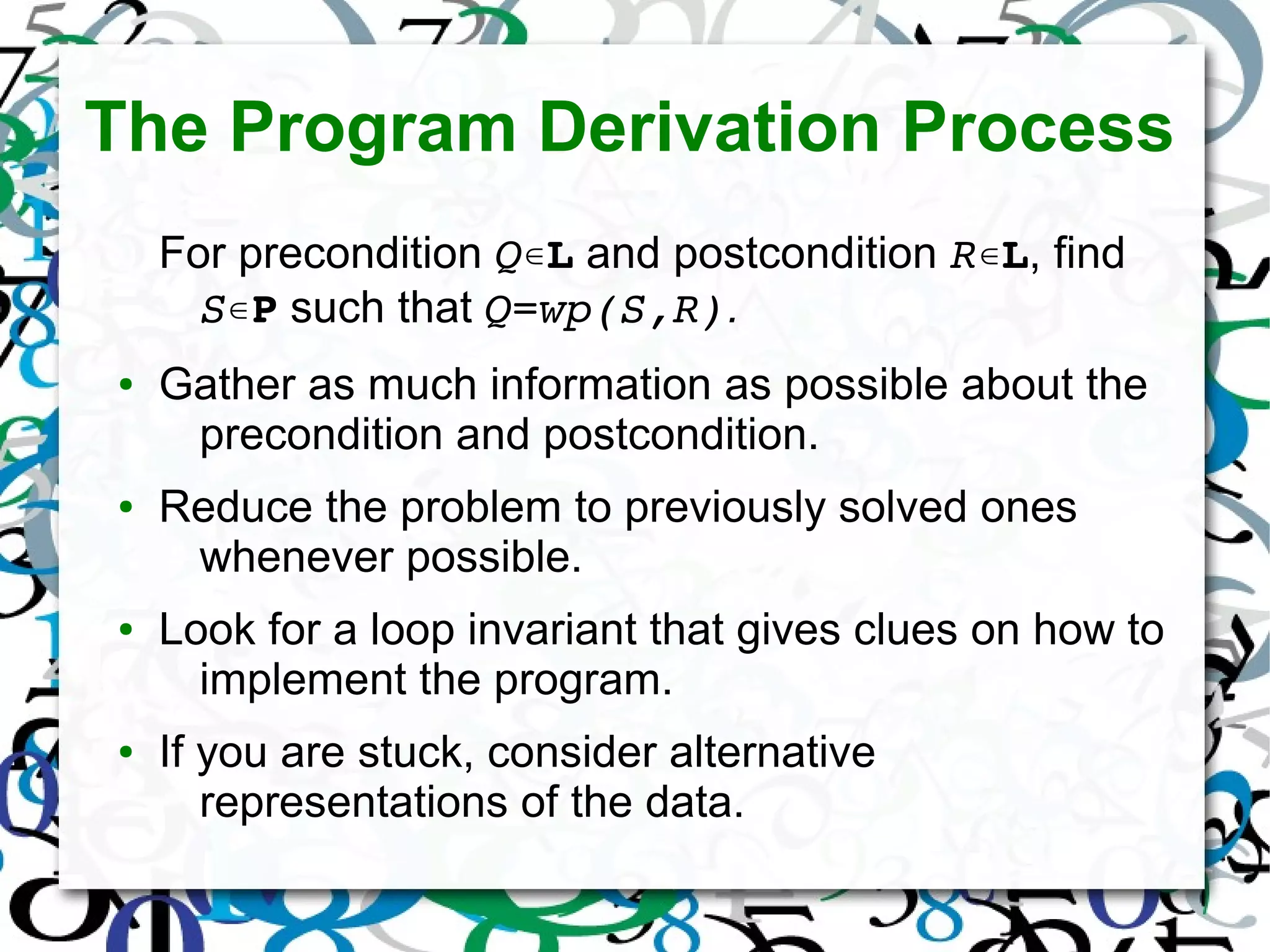
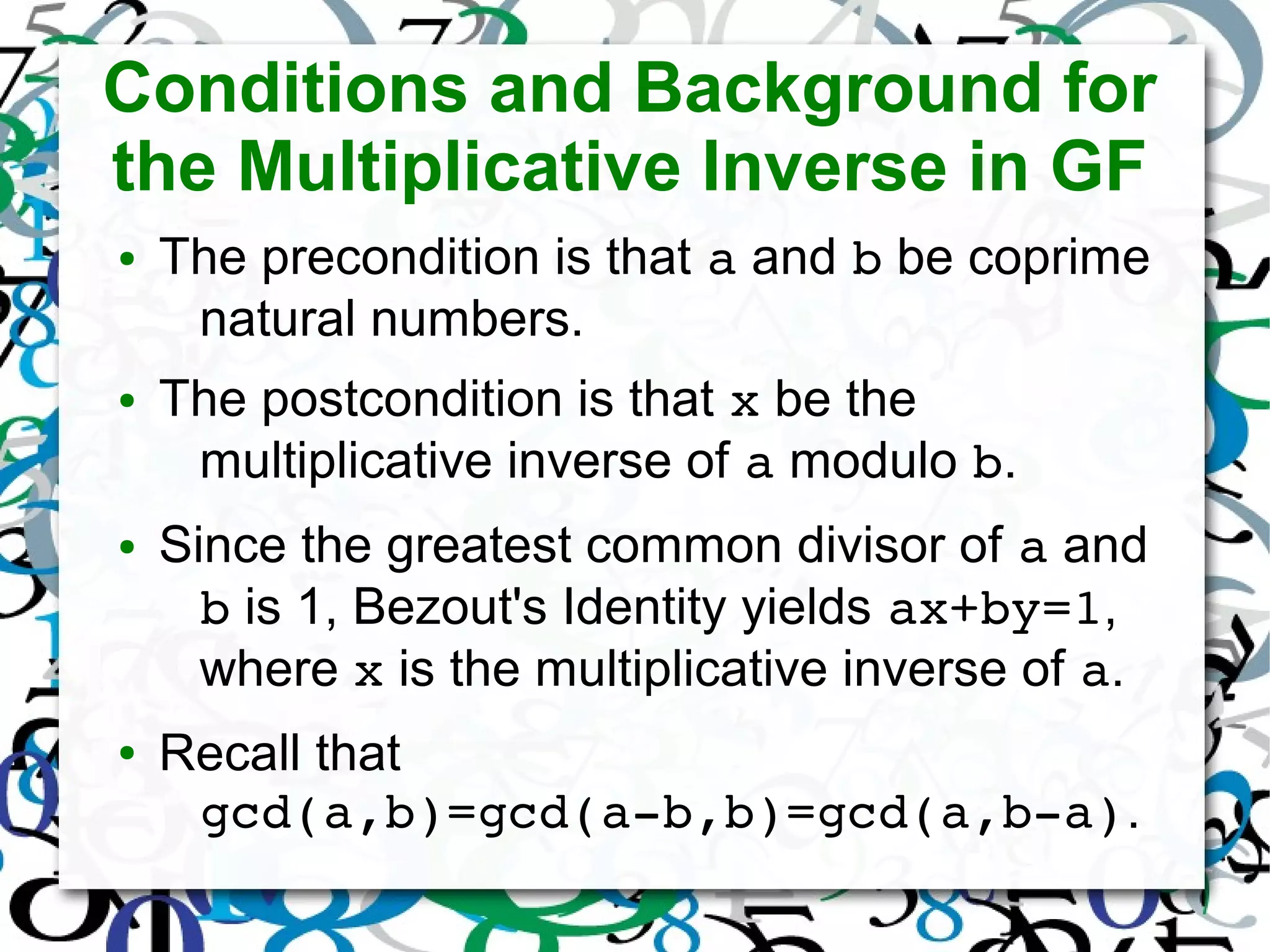
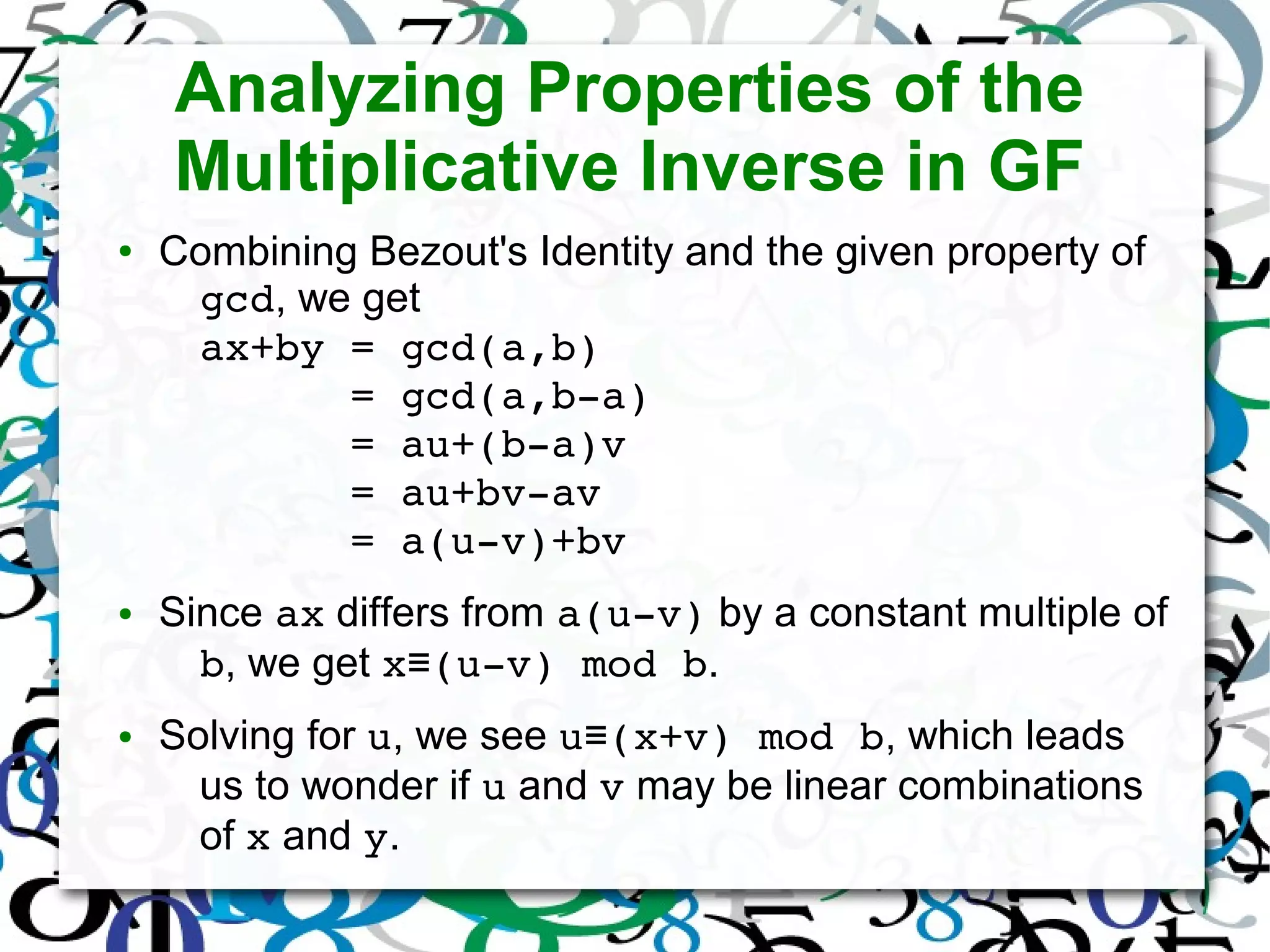
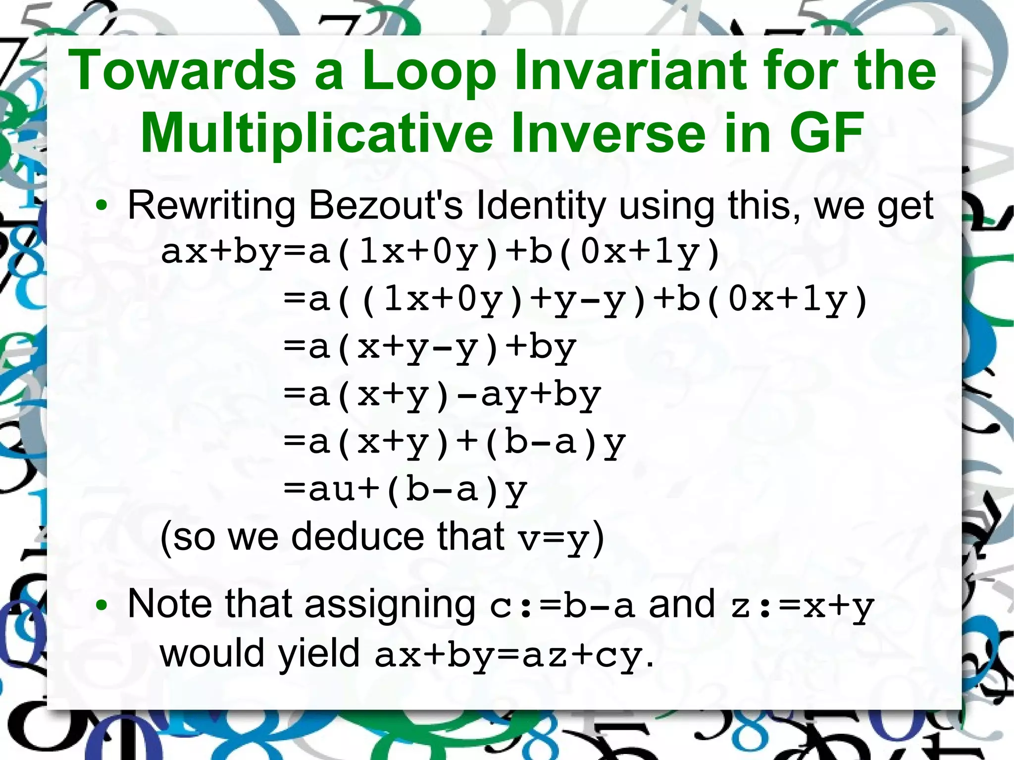

The document discusses matrix operations in Galois Fields (GF) and their significance in abstract algebra, particularly the properties of finite fields and the concept of program derivation. It covers foundational concepts such as the weakest precondition predicate transformer and various algorithms for calculating multiplicative inverses, matrix products, determinants, cofactor matrices, and matrix inverses, all within the context of GF. Additionally, it highlights the applications of matrices over GF in fields such as information theory, cryptography, and digital signal processing.