Probability and statistics- Understanding

Basic Biostat 5: Probability Concepts 1
Chapter 5:
Probability Concepts

In Chapter 5:
5.1 What is Probability?
5.2 Types of Random Variables
5.3 Discrete Random Variables
5.4 Continuous Random Variables
5.5 More Rules and Properties of Probability

Definitions
• Random variable ≡ a numerical quantity that
takes on different values depending on chance
• Population ≡ the set of all possible values for a
random variable
• Event ≡ an outcome or set of outcomes
• Probability ≡ the relative frequency of an
event in the population … alternatively…
the proportion of times an event is
expected to occur in the long run

Example
• In a given year: 42,636
traffic fatalities (events)
in a population of N =
293,655,000
• Random sample
population
• Probability of event
= relative freq in pop
= 42,636 / 293,655,000
= .0001452
≈ 1 in 6887

Example: Probability
• Assume, 20% of population has a condition
• Repeatedly sample population
• The proportion of observations positive for
the condition approaches 0.2 after a very
large number of trials

Random Variables
• Random variable ≡ a numerical quantity
that takes on different values depending
on chance
• Two types of random variables
– Discrete random variables (countable set of
possible outcomes)
– Continuous random variable (unbroken
chain of possible outcomes)

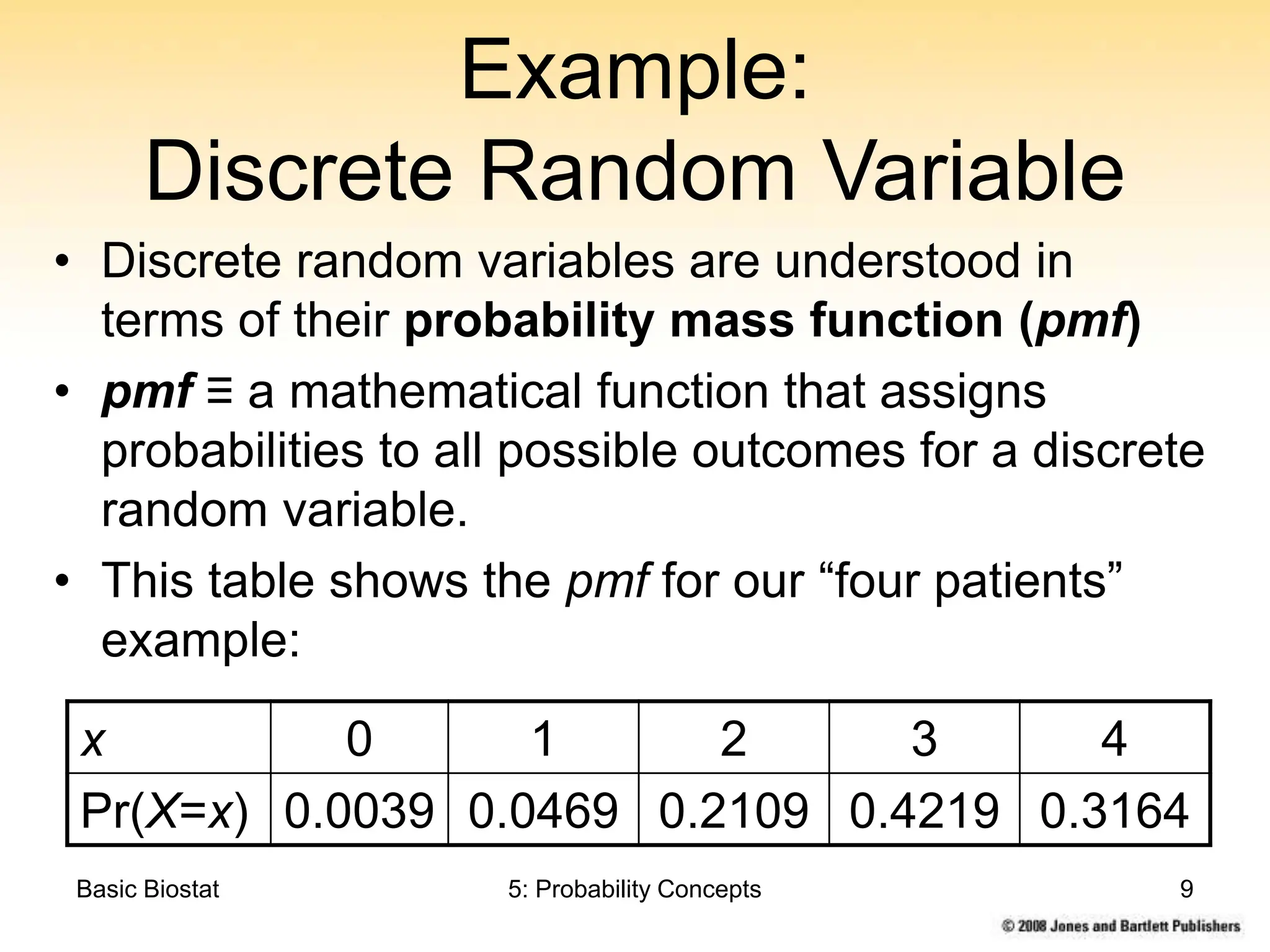
Example:
Discrete Random Variable
• Treat 4 patients with a
drug that is 75% effective
• Let X ≡ the [variable]
number of patients that
respond to treatment
• X is a discrete random
variable can be either 0,
1, 2, 3, or 4 (a countable
set of possible outcomes)

Example:
Discrete Random Variable
• Discrete random variables are understood in
terms of their probability mass function (pmf)
• pmf ≡ a mathematical function that assigns
probabilities to all possible outcomes for a discrete
random variable.
• This table shows the pmf for our “four patients”
example:
x 0 1 2 3 4
Pr(X=x) 0.0039 0.0469 0.2109 0.4219 0.3164

The “four patients” pmf can also be
shown graphically

Area on pmf = Probability
• Areas under pmf
graphs correspond
to probability
• For example:
Pr(X = 2)
= shaded rectangle
= height × base
= .2109 × 1.0
= .2109
“Four patients” pmf

Example:
Continuous Random Variable
• Continuous random
variables have an
infinite set of possible
outcomes
• Example: generate
random numbers with
this spinner 
• Outcomes form a
continuum between 0
and 1

Example
• probability density
function (pdf) ≡ a
mathematical function
that assigns probabilities
for continuous random
variables
• The probability of any
exact value is 0
• BUT, the probability of a
range is the area under
the pdf “curve” (bottom)

Example
• Area = probabilities
• The pdf for the random
spinner variable 
• The probability of a
value between 0 and
0.5 Pr(0 ≤ X ≤ 0.5)
= shaded rectangle
= height × base
= 1 × 0.5 = 0.5

pdfs come in various shapes
here are examples
Chi-square pdf Exercise 5.13 pdf
Normal pdf
Uniform pdf

Areas Under the Curve
• pdf curves are analogous
to probability histograms
• AREAS = probabilities
• Top figure: histogram,
ages ≤ 9 shaded
• Bottom figure: pdf,
ages ≤ 9 shaded
• Both represent proportion
of population ≤ 9

Properties of Probabilities
• Property 1. Probabilities are always between 0
and 1
• Property 2. The sample space (S) for a random
variable represents all possible outcomes and
must sum to 1 exactly.
• Property 3. The probability of the complement
of an event (“NOT the event”)= 1 MINUS the
probability of the event.
• Property 4. Probabilities of disjoint events can
be added.

Properties of Probabilities
In symbols
• Property 1. 0 ≤ Pr(A) ≤ 1
• Property 2. Pr(S) = 1
• Property 3. Pr(Ā) = 1 – Pr(A),
Ā represents the complement of A
• Property 4. Pr(A or B) = Pr(A) + Pr(B)
when A and B are disjoint

Properties 1 & 2 Illustrated
Property 1. Note that all
probabilities are between
0 and 1.
Property 2. The sample
space sums to 1:
Pr(S) = .0039 + .0469 +
.2109 + .4219 + .3164 = 1

Property 3 (“Complements”)
Let A ≡ 4 successes
Then, Ā ≡ “not A” = “3 or
fewer successes”
Property of complements:
Pr(Ā) = 1 – Pr(A)
= 1 – 0.3164
= 0.6836
Ā
A

Property 4 (Disjoint Events)
Let A represent 4 successes
Let B represent 3 successes
A & B are disjoint
The probability of observing 3
or 4:
Pr(A or B)
= Pr(A) + Pr(B)
= 0.3164 + 0.4129
= 0.7293
B A

Cumulative Probability
Left “tail”
• Cumulative probability
= probability of x or less
• Denoted Pr(X ≤ x)
• Corresponds to area in
left tail
• Example:
Pr(X ≤ 2)
= area in left tail
= .0039 + .0469 + .2109
= 0.2617
.0469
.2109
.0039

Right “tail”
• Probabilities greater than a
value are denoted Pr(X > x)
• Complement of cumulative
probability
• Corresponds to area in right
tail of distribution
• Example (4 patients pmf):
Pr (X > 3)
= complement of Pr(X ≤ 2)
= 1 - 0.2617
= .7389
.0469
.2109
.0039

Probability and statistics- Understanding

More Related Content

Similar to Probability and statistics- Understanding

Recently uploaded

Probability and statistics- Understanding

Editor's Notes