This document provides an introduction to key concepts in artificial intelligence including uncertainty, probability, possible worlds, unconditional and conditional probability, Bayes' rule, random variables, probability distributions, independence, Bayesian networks, and approximate inference techniques like sampling and likelihood weighting. It defines key terms and provides examples to illustrate probabilistic reasoning and how to compute probabilities and inferences in Bayesian networks.

1. Introduction to
Artificial Intelligence

2. Uncertainty

6. Probability

7. ω
Possible Worlds

8. P(ω)

9. 0 ≤ P(ω) ≤ 1

10. ∑ P(ω) = 1
ω∈Ω

11. 1 1 1 1 1 1
6 6 6 6 6 6

12. P( ) =
1
6

15. 2 3 4 5
3 4 5 6
4 5 6 7
5 6 7 8
6 7 8 9
7 8 9 10
6
7
8
9
10
1
1
7
8
9
10
1
1
12

16. 2 3 4 5
3 4 5 6
4 5 6 7
5 6 7 8
6 7 8 9
7 8 9 10
6
7
8
9
10
1
1
7
8
9
10
1
1
12

17. 2 3 4 5
3 4 5 6
4 5 6 7
5 6 7 8
6 7 8 9
7 8 9 10
6
7
8
9
10
1
1
7
8
9
10
1
1
12

18. P(sum to 7) =
P(sum to 12) =
1
36
6
=
1
36 6

19. unconditional probability
degree of belief in a proposition
in the absence of any other evidence

20. conditional probability
degree of belief in a proposition
given some evidence that has already
been revealed

21. conditional probability
P(a | b)

22. P(rain today | rain yesterday)

23. P(route change | traffic conditions)

24. P(disease | test results)

25. P(a|b) =
P(a ∧b)
P(b)

26. P(sum 12 | )

28. 6
P( ) =
1

29. 1
P( ) =
6
36
P(sum 12) =
1
6
P(sum 12 | )=
1

30. P(a|b) =
P(a ∧b)
P(b)
P(a ∧b) = P(b)P(a|b)
P(a ∧b) = P(a)P(b|a)

31. random variable
a variable in probability theory with a
domain of possible values it can take on

32. random variable
Roll
{1, 2, 3, 4, 5, 6}

33. random variable
Weather
{sun, cloud, rain, wind, snow}

34. random variable
Traffic
{none, light, heavy}

35. random variable
Flight
{on time, delayed, cancelled}

36. probability distribution
P(Flight = on time) = 0.6
P(Flight = delayed) = 0.3
P(Flight = cancelled) = 0.1

37. probability distribution
P(Flight) = ⟨0.6, 0.3, 0.1⟩

38. independence
the knowledge that one event occurs does
not affect the probability of the other event

39. independence
P(a ∧b) = P(a)P(b|a)

40. independence
P(a ∧b) = P(a)P(b)

41. independence
P( ) = P( )P( )
=
1
⋅
1
=
1
6 6 36

42. independence
P( ) ≠ P( )P( )
=
1
⋅
1
=
1
6 6 36

43. independence
P( ) ≠ P( )P( | )
6
=
1
⋅0 = 0

44. Bayes' Rule

45. P(a ∧b) = P(b) P(a|b)
P(a ∧b) P(a) P(b|a)

46. P(a) P(b|a) = P(b) P(a|b)

47. P(b|a) =
P(b) P(a|b)
P(a)
Bayes' Rule

48. P(b|a) =
P(a|b) P(b)
P(a)
Bayes' Rule

49. PM
AM
Given clouds in the morning,
what's the probability of rain in the afternoon?
• 80% of rainy afternoons start with cloudy
mornings.
• 40% of days have cloudy mornings.
• 10% of days have rainy afternoons.

50. P(rain|clouds) =
P(clouds|rain)P(rain)
P(clouds)
=
(.8)(.1)
.4
= 0.2

51. Knowing
P(cloudy morning | rainy afternoon)
we can calculate
P(rainy afternoon | cloudy morning)

52. Knowing
P(visible effect | unknown cause)
we can calculate
P(unknown cause | visible effect)

53. Knowing
P(medical test result | disease)
we can calculate
P(disease | medical test result)

54. Knowing
P(blurry text | counterfeit bill)
we can calculate
P(counterfeit bill | blurry text)

55. Joint Probability

56. C = cloud C = ¬cloud
0.4 0.6
AM
R = rain R = ¬rain
C = cloud 0.08 0.32
C = ¬cloud 0.02 0.58
PM
R = rain R = ¬rain
0.1 0.9
PM
AM

57. P(C | rain)
R = rain R = ¬rain
C = cloud 0.08 0.32
C = ¬cloud 0.02 0.58
P(C | rain) =
P(C, rain)
P(rain)
= αP(C, rain)
= α⟨0.08, 0.02⟩ = ⟨0.8, 0.2⟩

58. Probability Rules

59. P(¬a) = 1 −P(a)
Negation

60. P(a ∨b) = P(a) + P(b) −P(a ∧b)
Inclusion-Exclusion

61. P(a) = P(a, b) + P(a, ¬b)
Marginalization

62. P(X = xi) = ∑ P(X = xi, Y = yj)
j
Marginalization

63. Marginalization
R = rain R = ¬rain
C = cloud 0.08 0.32
C = ¬cloud 0.02 0.58
P(C = cloud)
= P(C = cloud, R = rain) + P(C = cloud, R = ¬rain)
= 0.08 + 0.32
= 0.40

64. P(a) = P(a|b)P(b) + P(a|¬b)P(¬b)
Conditioning

65. P(X = xi) = ∑ P(X = xi |Y = yj)P(Y = yj)
j
Conditioning

66. Bayesian Networks

67. Bayesian network
data structure that represents the
dependencies among random variables

68. Bayesian network
• directed graph
• each node represents a random variable
• arrow from X to Y means X is a parent of Y
• each node X has probability distribution
P(X | Parents(X))

69. Rain
{none, light, heavy}
Maintenance
{yes, no}
Train
{on time, delayed}
Appointment
{attend, miss}

70. Rain
{none, light, heavy}
none light heavy
0.7 0.2 0.1

71. Rain
{none, light, heavy}
Maintenance
{yes, no}
R yes no
none 0.4 0.6
light 0.2 0.8
heavy 0.1 0.9

72. Rain
{none, light, heavy}
Maintenance
{yes, no}
Train
{on time, delayed}
R M on time delayed
none yes 0.8 0.2
none no 0.9 0.1
light yes 0.6 0.4
light no 0.7 0.3
heavy yes 0.4 0.6
heavy no 0.5 0.5

73. Maintenance
{yes, no}
Train
{on time, delayed}
Appointment
{attend, miss}
T attend miss
on time 0.9 0.1
delayed 0.6 0.4

74. Rain
{none, light, heavy}
Maintenance
{yes, no}
Train
{on time, delayed}
Appointment
{attend, miss}

75. Appointment
{attend, miss}
Maintenance
{yes, no}
Train
{on time, delayed}
Rain
{none, light, heavy}
P(light)
P(light)
Computing Joint Probabilities

76. Appointment
{attend, miss}
Maintenance
{yes, no}
Train
{on time, delayed}
Rain
{none, light, heavy}
P(light, no)
P(light) P(no | light)
Computing Joint Probabilities

77. Appointment
{attend, miss}
Maintenance
{yes, no}
Train
{on time, delayed}
Rain
{none, light, heavy}
P(light, no, delayed)
P(light) P(no | light) P(delayed | light, no)
Computing Joint Probabilities

78. Appointment
{attend, miss}
Maintenance
{yes, no}
Train
{on time, delayed}
Rain
{none, light, heavy}
P(light, no, delayed, miss)
P(light) P(no | light) P(delayed | light, no) P(miss | delayed)
Computing Joint Probabilities

79. Inference

80. Inference
• Query X: variable for which to compute distribution
• Evidence variables E: observed variables for event e
• Hidden variables Y: non-evidence, non-query variable.
• Goal: Calculate P(X | e)

81. Appointment
{attend, miss}
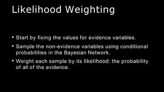
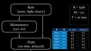
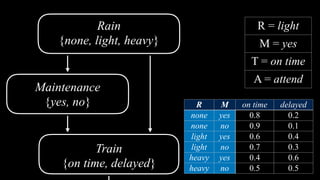
Train
{on time, delayed}
Maintenance
{yes, no}
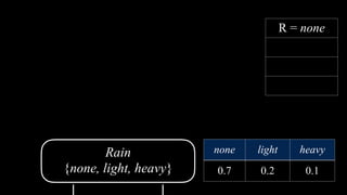
Rain
{none, light, heavy}
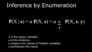
P(Appointment | light, no)
= α P(Appointment, light, no)
= α [P(Appointment, light, no, on time)
+ P(Appointment, light, no, delayed)]

82. Inference by Enumeration
P(X | e) = α P(X, e) = α ∑ P(X, e, y)
y
X is the query variable.
e is the evidence.
y ranges over values of hidden variables.
α normalizes the result.

83. Approximate Inference

84. Sampling

85. Rain
{none, light, heavy}
Maintenance
{yes, no}
Train
{on time, delayed}
Appointment
{attend, miss}

86. Rain
{none, light, heavy}
none light heavy
0.7 0.2 0.1
R = none

87. Rain
{none, light, heavy}
Maintenance
{yes, no}
R yes no
none 0.4 0.6
light 0.2 0.8
heavy 0.1 0.9
R = none
M = yes

88. Rain
{none, light, heavy}
Maintenance
{yes, no}
Train
{on time, delayed}
R M on time delayed
none yes 0.8 0.2
none no 0.9 0.1
light yes 0.6 0.4
light no 0.7 0.3
heavy yes 0.4 0.6
heavy no 0.5 0.5
R = none
M = yes
T = on time

89. Maintenance
{yes, no}
Train
{on time, delayed}
Appointment
{attend, miss}
T attend miss
on time 0.9 0.1
delayed 0.6 0.4
R = none
M = yes
T = on time
A = attend

90. R = none
M = yes
T = on time
A = attend

91. R = none
M = yes
T = on time
A = attend
R = none
M = no
T = on time
A = attend
R = light
M = yes
T = delayed
A = attend
R = light
M = no
T = on time
A = miss
R = none
M = yes
T = on time
A = attend
R = none
M = yes
T = on time
A = attend
R = heavy
M = no
T = delayed
A = miss
R = light
M = no
T = on time
A = attend

92. P(Train = on time) ?

93. R = none
M = yes
T = on time
A = attend
R = none
M = no
T = on time
A = attend
R = light
M = yes
T = delayed
A = attend
R = light
M = no
T = on time
A = miss
R = none
M = yes
T = on time
A = attend
R = none
M = yes
T = on time
A = attend
R = heavy
M = no
T = delayed
A = miss
R = light
M = no
T = on time
A = attend

94. R = none
M = yes
T = on time
A = attend
R = none
M = no
T = on time
A = attend
R = light
M = yes
T = delayed
A = attend
R = light
M = no
T = on time
A = miss
R = none
M = yes
T = on time
A = attend
R = none
M = yes
T = on time
A = attend
R = heavy
M = no
T = delayed
A = miss
R = light
M = no
T = on time
A = attend

95. P(Rain = light | Train = on time) ?

96. R = none
M = yes
T = on time
A = attend
R = none
M = no
T = on time
A = attend
R = light
M = yes
T = delayed
A = attend
R = light
M = no
T = on time
A = miss
R = none
M = yes
T = on time
A = attend
R = none
M = yes
T = on time
A = attend
R = heavy
M = no
T = delayed
A = miss
R = light
M = no
T = on time
A = attend

97. R = none
M = yes
T = on time
A = attend
R = none
M = no
T = on time
A = attend
R = light
M = yes
T = delayed
A = attend
R = light
M = no
T = on time
A = miss
R = none
M = yes
T = on time
A = attend
R = none
M = yes
T = on time
A = attend
R = heavy
M = no
T = delayed
A = miss
R = light
M = no
T = on time
A = attend

98. R = none
M = yes
T = on time
A = attend
R = none
M = no
T = on time
A = attend
R = light
M = yes
T = delayed
A = attend
R = light
M = no
T = on time
A = miss
R = none
M = yes
T = on time
A = attend
R = none
M = yes
T = on time
A = attend
R = heavy
M = no
T = delayed
A = miss
R = light
M = no
T = on time
A = attend

99. Rejection Sampling

100. Likelihood Weighting

101. Likelihood Weighting
• Start by fixing the values for evidence variables.
• Sample the non-evidence variables using conditional
probabilities in the Bayesian Network.
• Weight each sample by its likelihood: the probability
of all of the evidence.

102. P(Rain = light | Train = on time) ?

103. Rain
{none, light, heavy}
Maintenance
{yes, no}
Train
{on time, delayed}
Appointment
{attend, miss}

104. Rain
{none, light, heavy}
none light heavy
0.7 0.2 0.1
R = light
T = on time

105. Rain
{none, light, heavy}
Maintenance
{yes, no}
R yes no
none 0.4 0.6
light 0.2 0.8
heavy 0.1 0.9
R = light
M = yes
T = on time

106. Rain
{none, light, heavy}
Maintenance
{yes, no}
Train
{on time, delayed}
R M on time delayed
none yes 0.8 0.2
none no 0.9 0.1
light yes 0.6 0.4
light no 0.7 0.3
heavy yes 0.4 0.6
heavy no 0.5 0.5
R = light
M = yes
T = on time

107. Maintenance
{yes, no}
Train
{on time, delayed}
Appointment
{attend, miss}
T attend miss
on time 0.9 0.1
delayed 0.6 0.4
R = light
M = yes
T = on time
A = attend

108. Rain
{none, light, heavy}
Maintenance
{yes, no}
Train
{on time, delayed}
R M on time delayed
none yes 0.8 0.2
none no 0.9 0.1
light yes 0.6 0.4
light no 0.7 0.3
heavy yes 0.4 0.6
heavy no 0.5 0.5
R = light
M = yes
T = on time
A = attend

109. Rain
{none, light, heavy}
Maintenance
{yes, no}
Train
{on time, delayed}
R M on time delayed
none yes 0.8 0.2
none no 0.9 0.1
light yes 0.6 0.4
light no 0.7 0.3
heavy yes 0.4 0.6
heavy no 0.5 0.5
R = light
M = yes
T = on time
A = attend

110. Uncertainty over Time

111. Xt: Weather at time t

112. Markov assumption
the assumption that the current state
depends on only a finite fixed number of
previous states

113. Markov Chain

114. Markov chain
a sequence of random variables where the
distribution of each variable follows the
Markov assumption

115. 0.8 0.2
0.3 0.7
Today (Xt)
Tomorrow (Xt+1)
Transition Model

116. X0 X1 X2 X3 X4

117. Sensor Models

118. Hidden State Observation
robot's position robot's sensor data
words spoken audio waveforms
user engagement website or app analytics
weather umbrella

119. Hidden Markov Models

120. Hidden Markov Model
a Markov model for a system with hidden
states that generate some observed event

121. 0.2 0.8
0.9 0.1
State (Xt)
Observation (Et)
Sensor Model

122. sensor Markov assumption
the assumption that the evidence variable
depends only the corresponding state

123. X0 X1 X2 X3 X4
E0 E1 E2 E3 E4

124. Task Definition
filtering
given observations from start until now,
calculate distribution for current state
prediction
given observations from start until now,
calculate distribution for a future state
smoothing
given observations from start until now,
calculate distribution for past state
most likely
explanation
given observations from start until now,
calculate most likely sequence of states

125. Uncertainty

126. Introduction to
Artificial Intelligence
with Python