The document outlines the third edition of 'Principles of Distributed Database Systems' by M. Tamer Özsu and Patrick Valduriez, reflecting significant updates and changes in the field of distributed data management. Key revisions include detailed discussions on database integration, data replication protocols, peer-to-peer data management, and web data management, as well as new topics such as stream data management and cloud computing. The book maintains its core principles while addressing emerging technologies and changes within distributed systems, providing a comprehensive resource for students and professionals in the area.
![connection with any form of information storage and retrieval,
electronic adaptation, computer, software,
or by similar or dissimilar methodology now known or hereafter
developed is forbidden.
The use in this publication of trade names, trademarks, service
marks, and similar terms, even if they
are not identified as such, is not to be taken as an expression of
opinion as to whether or not they are
subject to proprietary rights.
Printed on acid-free paper
Springer is part of Springer Science+Business Media
(www.springer.com)
Springer New York Dordrecht Heidelberg London
M. Tamer Özsu
David R. Cheriton School of
Computer Science
University of Waterloo
Waterloo Ontario
Canada N2L 3G1
ISBN 978-1-4419-8833-1 e-ISBN 978-1-4419-8834-8
DOI 10.1007/978-1-4419-8834-8
This book was previously published by: Pearson Education, Inc.
[email protected]
Library of Congress Control Number: 2011922491
© Springer Science+Business Media, LLC 2011
Patrick Valduriez](https://image.slidesharecdn.com/principlesofdistributeddatabasesystems-221119021321-940a108d/85/Principles-of-Distributed-Database-Systems-docx-2-320.jpg)
![LIRMM
34392 Montpellier Cedex
France
[email protected]
INRIA
161 rue Ada
To my family
and my parents
M.T.Ö.
To Esther, my daughters Anna, Juliette and
Sarah, and my parents
P.V.
Preface
It has been almost twenty years since the first edition of this
book appeared, and ten
years since we released the second edition. As one can imagine,
in a fast changing
area such as this, there have been significant changes in the
intervening period.
Distributed data management went from a potentially significant
technology to one
that is common place. The advent of the Internet and the World
Wide Web have](https://image.slidesharecdn.com/principlesofdistributeddatabasesystems-221119021321-940a108d/85/Principles-of-Distributed-Database-Systems-docx-3-320.jpg)


![M. Tamer Özsu ([email protected])
Patrick Valduriez ([email protected])
November 2010
Contents
1 Introduction . . . . . . . . . . . . . . . . . . . . . . . . . . . . . . . . . . . . .
. . . . . . . . . . . . . . 1
1.1 Distributed Data Processing . . . . . . . . . . . . . . . . . . . . . . . .
. . . . . . . . . . 2
1.2 What is a Distributed Database System? . . . . . . . . . . . . . . .
. . . . . . . . 3
1.3 Data Delivery Alternatives . . . . . . . . . . . . . . . . . . . . . . . .
. . . . . . . . . . . 5
1.4 Promises of DDBSs . . . . . . . . . . . . . . . . . . . . . . . . . . . . . .
. . . . . . . . . . 7
1.4.1 Transparent Management of Distributed and Replicated
Data 7
1.4.2 Reliability Through Distributed Transactions . . . . . . . . . .
. . . 12
1.4.3 Improved Performance . . . . . . . . . . . . . . . . . . . . . . . . . .
. . . . . . 14
1.4.4 Easier System Expansion . . . . . . . . . . . . . . . . . . . . . . . .
. . . . . . 15
1.5 Complications Introduced by Distribution . . . . . . . . . . . . . .
. . . . . . . . 16
1.6 Design Issues . . . . . . . . . . . . . . . . . . . . . . . . . . . . . . . . . .
. . . . . . . . . . . . 16
1.6.1 Distributed Database Design . . . . . . . . . . . . . . . . . . . . . .](https://image.slidesharecdn.com/principlesofdistributeddatabasesystems-221119021321-940a108d/85/Principles-of-Distributed-Database-Systems-docx-11-320.jpg)


![vague.
In this book we define distributed processing in such a way that
it leads to a
definition of a distributed database system. The working
definition we use for a
distributed computing system states that it is a number of
autonomous processing
elements (not necessarily homogeneous) that are interconnected
by a computer
network and that cooperate in performing their assigned tasks.
The “processing
element” referred to in this definition is a computing device that
can execute a
program on its own. This definition is similar to those given in
distributed systems
textbooks (e.g., [Tanenbaum and van Steen, 2002] and [Colouris
et al., 2001]).
A fundamental question that needs to be asked is: What is being
distributed?
One of the things that might be distributed is the processing
logic. In fact, the
definition of a distributed computing system given above
implicitly assumes that the](https://image.slidesharecdn.com/principlesofdistributeddatabasesystems-221119021321-940a108d/85/Principles-of-Distributed-Database-Systems-docx-50-320.jpg)


![is initiated by a server push in the absence of any specific
request from clients.
The main difficulty of the push-based approach is in deciding
which data would be
of common interest, and when to send them to clients –
alternatives are periodic,
irregular, or conditional. Thus, the usefulness of server push
depends heavily upon
the accuracy of a server to predict the needs of clients. In push-
based mode, servers
disseminate information to either an unbounded set of clients
(random broadcast)
who can listen to a medium or selective set of clients
(multicast), who belong to some
categories of recipients that may receive the data.
The hybrid mode of data delivery combines the client-pull and
server-push mech-
anisms. The continuous (or continual) query approach (e.g.,
[Liu et al., 1996],[Terry
et al., 1992],[Chen et al., 2000],[Pandey et al., 2003]) presents
one possible way of
combining the pull and push modes: namely, the transfer of
information from servers
to clients is first initiated by a client pull (by posing the query),](https://image.slidesharecdn.com/principlesofdistributeddatabasesystems-221119021321-940a108d/85/Principles-of-Distributed-Database-Systems-docx-61-320.jpg)


![server sends data
to a number of clients. Note that we are not referring here to a
specific protocol;
one-to-many communication may use a multicast or broadcast
protocol.
We should note that this characterization is subject to
considerable debate. It is
not clear that every point in the design space is meaningful.
Furthermore, specifi-
cation of alternatives such as conditional and periodic (which
may make sense) is
difficult. However, it serves as a first-order characterization of
the complexity of
emerging distributed data management systems. For the most
part, in this book, we
are concerned with pull-only, ad hoc data delivery systems,
although examples of
other approaches are discussed in some chapters.
1.4 Promises of DDBSs
Many advantages of DDBSs have been cited in literature,
ranging from sociological
reasons for decentralization [D’Oliviera, 1977] to better](https://image.slidesharecdn.com/principlesofdistributeddatabasesystems-221119021321-940a108d/85/Principles-of-Distributed-Database-Systems-docx-65-320.jpg)


![[Gray, 1989]. He proposes a remote procedure call mechanism
between the requestor
users and the server DBMSs whereby the users would direct
their queries to a specific
DBMS. This is indeed the approach commonly taken by
client/server systems that
we discuss shortly.
What has not yet been discussed is who is responsible for
providing these services.
It is possible to identify three distinct layers at which the
transparency services can be
provided. It is quite common to treat these as mutually
exclusive means of providing
the service, although it is more appropriate to view them as
complementary.
12 1 Introduction
We could leave the responsibility of providing transparent
access to data resources
to the access layer. The transparency features can be built into
the user language,](https://image.slidesharecdn.com/principlesofdistributeddatabasesystems-221119021321-940a108d/85/Principles-of-Distributed-Database-Systems-docx-80-320.jpg)


![Committee (SPARC). The mission of the study group was to
study the feasibility
of setting up standards in this area, as well as determining
which aspects should be
standardized if it was feasible. The study group issued its
interim report in 1975
[ANSI/SPARC, 1975], and its final report in 1977 [Tsichritzis
and Klug, 1978].
The architectural framework proposed in these reports came to
be known as the
“ANSI/SPARC architecture,” its full title being
“ANSI/X3/SPARC DBMS Frame-
work.” The study group proposed that the interfaces be
standardized, and defined
an architectural framework that contained 43 interfaces, 14 of
which would deal
with the physical storage subsystem of the computer and
therefore not be considered
essential parts of the DBMS architecture.
A simplified version of the ANSI/SPARC architecture is
depicted in Figure 1.8.
There are three views of data: the external view, which is that
of the end user, who
might be a programmer; the internal view, that of the system or](https://image.slidesharecdn.com/principlesofdistributeddatabasesystems-221119021321-940a108d/85/Principles-of-Distributed-Database-Systems-docx-115-320.jpg)

![1977]. As such, it is supposed to represent the data and the
relationships among data
without considering the requirements of individual applications
or the restrictions
of the physical storage media. In reality, however, it is not
possible to ignore these
1.7 Distributed DBMS Architecture 23
requirements completely, due to performance reasons. The
transformation between
these three levels is accomplished by mappings that specify how
a definition at one
level can be obtained from a definition at another level.
This perspective is important, because it provides the basis for
data independence
that we discussed earlier. The separation of the external
schemas from the conceptual
schema enables logical data independence, while the separation
of the conceptual
schema from the internal schema allows physical data
independence.](https://image.slidesharecdn.com/principlesofdistributeddatabasesystems-221119021321-940a108d/85/Principles-of-Distributed-Database-Systems-docx-117-320.jpg)


![independently exe-
cute transactions, and whether one is allowed to modify them.
Requirements of an
autonomous system have been specified as follows [Gligor and
Popescu-Zeletin,
1986]:
1. The local operations of the individual DBMSs are not
affected by their partic-
ipation in the distributed system.
26 1 Introduction
2. The manner in which the individual DBMSs process queries
and optimize
them should not be affected by the execution of global queries
that access
multiple databases.
3. System consistency or operation should not be compromised
when individual
DBMSs join or leave the distributed system.](https://image.slidesharecdn.com/principlesofdistributeddatabasesystems-221119021321-940a108d/85/Principles-of-Distributed-Database-Systems-docx-126-320.jpg)
![On the other hand, the dimensions of autonomy can be specified
as follows [Du
and Elmagarmid, 1989]:
1. Design autonomy: Individual DBMSs are free to use the data
models and
transaction management techniques that they prefer.
2. Communication autonomy: Each of the individual DBMSs is
free to make its
own decision as to what type of information it wants to provide
to the other
DBMSs or to the software that controls their global execution.
3. Execution autonomy: Each DBMS can execute the
transactions that are sub-
mitted to it in any way that it wants to.
We will use a classification that covers the important aspects of
these features.
One alternative is tight integration, where a single-image of the
entire database
is available to any user who wants to share the information,
which may reside in
multiple databases. From the users’ perspective, the data are](https://image.slidesharecdn.com/principlesofdistributeddatabasesystems-221119021321-940a108d/85/Principles-of-Distributed-Database-Systems-docx-127-320.jpg)


![distributed system architecture, where sites are organized as
specialized servers
rather than as general-purpose computers.
The original idea, which is to offload the database management
functions to a
special server, dates back to the early 1970s [Canaday et al.,
1974]. At the time, the
computer on which the database system was run was called the
database machine,
database computer, or backend computer, while the computer
that ran the applica-
tions was called the host computer. More recent terms for these
are the database
server and application server, respectively. Figure 1.12
illustrates a simple view of
the database server approach, with application servers
connected to one database
server via a communication network.
The database server approach, as an extension of the classical
client/server archi-
tecture, has several potential advantages. First, the single focus
on data management
makes possible the development of specific techniques for](https://image.slidesharecdn.com/principlesofdistributeddatabasesystems-221119021321-940a108d/85/Principles-of-Distributed-Database-Systems-docx-142-320.jpg)


![conceptual schema. In
the case of logically integrated distributed DBMSs, the global
conceptual schema
defines the conceptual view of the entire database, while in the
case of distributed
multi-DBMSs, it represents only the collection of some of the
local databases that
each local DBMS wants to share. The individual DBMSs may
choose to make some
of their data available for access by others (i.e., federated
database architectures) by
defining an export schema [Heimbigner and McLeod, 1985].
Thus the definition of a
global database is different in MDBSs than in distributed
DBMSs. In the latter, the
global database is equal to the union of local databases, whereas
in the former it is
only a (possibly proper) subset of the same union. In a MDBS,
the GCS (which is
also called a mediated schema) is defined by integrating either
the external schemas
of local autonomous databases or (possibly parts of their) local
conceptual schemas.
Furthermore, users of a local DBMS define their own views on](https://image.slidesharecdn.com/principlesofdistributeddatabasesystems-221119021321-940a108d/85/Principles-of-Distributed-Database-Systems-docx-160-320.jpg)


![vides a layer of software that runs on top of these individual
DBMSs and provides
users with the facilities of accessing various databases (Figure
1.17). Note that in a
distributed MDBS, the multi-DBMS layer may run on multiple
sites or there may be
central site where those services are offered. Also note that as
far as the individual
DBMSs are concerned, the MDBS layer is simply another
application that submits
requests and receives answers.
A popular implementation architecture for MDBSs is the
mediator/wrapper ap-
proach (Figure 1.18) [Wiederhold, 1992]. A mediator “is a
software module that
exploits encoded knowledge about certain sets or subsets of data
to create information
for a higher layer of applications.” Thus, each mediator
performs a particular function
with clearly defined interfaces. Using this architecture to
implement a MDBS, each
module in the multi-DBMS layer of Figure 1.17 is realized as a
mediator. Since
mediators can be built on top of other mediators, it is possible](https://image.slidesharecdn.com/principlesofdistributeddatabasesystems-221119021321-940a108d/85/Principles-of-Distributed-Database-Systems-docx-165-320.jpg)


![significant study in the past decade and very sophisticated
middleware systems have
been developed that provide advanced services for development
of distributed appli-
cations. The mediators that we discuss only represent a subset
of the functionality
provided by these systems.
1.8 Bibliographic Notes
There are not many books on distributed DBMSs. Ceri and
Pelagatti’s book [Ceri
and Pelagatti, 1983] was the first on this topic though it is now
dated. The book
by Bell and Grimson [Bell and Grimson, 1992] also provides an
overview of the
topics addressed here. In addition, almost every database book
now has a chapter on
distributed DBMSs. A brief overview of the technology is
provided in [Özsu and
Valduriez, 1997]. Our papers [Özsu and Valduriez, 1994, 1991]
provide discussions
of the state-of-the-art at the time they were written.
Database design is discussed in an introductory manner in](https://image.slidesharecdn.com/principlesofdistributeddatabasesystems-221119021321-940a108d/85/Principles-of-Distributed-Database-Systems-docx-168-320.jpg)
![[Levin and Morgan,
1975] and more comprehensively in [Ceri et al., 1987]. A
survey of the file distribu-
tion algorithms is given in [Dowdy and Foster, 1982]. Directory
management has not
been considered in detail in the research community, but
general techniques can be
found in Chu and Nahouraii [1975] and [Chu, 1976]. A survey
of query processing
1.8 Bibliographic Notes 39
USER
User
requests
System
responses
...](https://image.slidesharecdn.com/principlesofdistributeddatabasesystems-221119021321-940a108d/85/Principles-of-Distributed-Database-Systems-docx-169-320.jpg)
![Wrapper Wrapper Wrapper
Mediator Mediator
Mediator Mediator
DBMS DBMS DBMS DBMS
Fig. 1.18 Mediator/Wrapper Architecture
techniques can be found in [Sacco and Yao, 1982]. Concurrency
control algorithms
are reviewed in [Bernstein and Goodman, 1981] and [Bernstein
et al., 1987]. Dead-
lock management has also been the subject of extensive
research; an introductory
paper is [Isloor and Marsland, 1980] and a widely quoted paper
is [Obermarck,
1982]. For deadlock detection, good surveys are [Knapp, 1987]
and [Elmagarmid,
1986]. Reliability is one of the issues discussed in [Gray, 1979],
which is one of the
landmark papers in the field. Other important papers on this
topic are [Verhofstadt,
1978] and [Härder and Reuter, 1983]. [Gray, 1979] is also the](https://image.slidesharecdn.com/principlesofdistributeddatabasesystems-221119021321-940a108d/85/Principles-of-Distributed-Database-Systems-docx-170-320.jpg)
![first paper discussing
the issues of operating system support for distributed databases;
the same topic is
addressed in [Stonebraker, 1981]. Unfortunately, both papers
emphasize centralized
database systems.
There have been a number of architectural framework proposals.
Some of the inter-
esting ones include Schreiber’s quite detailed extension of the
ANSI/SPARC frame-
work which attempts to accommodate heterogeneity of the data
models [Schreiber,
1977], and the proposal by Mohan and Yeh [Mohan and Yeh,
1978]. As expected,
these date back to the early days of the introduction of
distributed DBMS technology.
The detailed component-wise system architecture given in
Figure 1.15 derives from
40 1 Introduction
[Rahimi, 1987]. An alternative to the classification that we](https://image.slidesharecdn.com/principlesofdistributeddatabasesystems-221119021321-940a108d/85/Principles-of-Distributed-Database-Systems-docx-171-320.jpg)
![provide in Figure 1.10
can be found in [Sheth and Larson, 1990].
Most of the discussion on architectural models for multi-
DBMSs is from [Özsu
and Barker, 1990]. Other architectural discussions on multi-
DBMSs are given in
[Gligor and Luckenbaugh, 1984], [Litwin, 1988], and [Sheth
and Larson, 1990]. All
of these papers provide overview discussions of various
prototype and commercial
systems. An excellent overview of heterogeneous and federated
database systems is
[Sheth and Larson, 1990].
Chapter 2
Background
As indicated in the previous chapter, there are two
technological bases for distributed
database technology: database management and computer
networks. In this chapter,
we provide an overview of the concepts in these two fields that](https://image.slidesharecdn.com/principlesofdistributeddatabasesystems-221119021321-940a108d/85/Principles-of-Distributed-Database-Systems-docx-172-320.jpg)


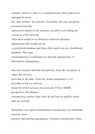
![P4 Manager 48
P3 Engineer 36
P3 Manager 40
PROJ
PNO PNAME BUDGET
P1 Instrumentation 150000
P2 Database Develop. 135000
P3 CAD/CAM 250000
P4 Maintenance 310000
Fig. 2.2 Sample Database Instance
known information (e.g., in the case of a newly hired
employee), while value “null”
for DUR means unknown. Supporting null values is an
important feature necessary
to deal with maybe queries [Codd, 1979].](https://image.slidesharecdn.com/principlesofdistributeddatabasesystems-221119021321-940a108d/85/Principles-of-Distributed-Database-Systems-docx-181-320.jpg)


![without these
problems. A relation with one or more of the above mentioned
anomalies is split into
two or more relations of a higher normal form. A relation is said
to be in a normal
form if it satisfies the conditions associated with that normal
form. Codd initially
defined the first, second, and third normal forms (1NF, 2NF,
and 3NF, respectively).
Boyce and Codd [Codd, 1974] later defined a modified version
of the third normal
form, commonly known as the Boyce-Codd normal form
(BCNF). This was followed
by the definition of the fourth (4NF) [Fagin, 1977] and fifth
normal forms (5NF)
[Fagin, 1979].
The normal forms are based on certain dependency structures.
BCNF and lower
normal forms are based on functional dependencies (FDs), 4NF
is based on multi-
valued dependencies, and 5NF is based on projection-join
dependencies. We only
introduce functional dependency, since that is the only relevant
one for the example](https://image.slidesharecdn.com/principlesofdistributeddatabasesystems-221119021321-940a108d/85/Principles-of-Distributed-Database-Systems-docx-184-320.jpg)


![relational calculus, on the other hand, is non-procedural; the
user only specifies the
relationships that should hold in the result. Both of these
languages were originally
proposed by Codd [1970], who also proved that they were
equivalent in terms of
expressive power [Codd, 1972].
2.1.3.1 Relational Algebra
Relational algebra consists of a set of operators that operate on
relations. Each
operator takes one or two relations as operands and produces a
result relation, which,
in turn, may be an operand to another operator. These
operations permit the querying
and updating of a relational database.
46 2 Background
ENO ENAME TITLE
E1 J. Doe Elect. Eng](https://image.slidesharecdn.com/principlesofdistributeddatabasesystems-221119021321-940a108d/85/Principles-of-Distributed-Database-Systems-docx-188-320.jpg)


![the second part of the
definition by the phrase “the corresponding attributes of the two
relations should be
defined over the same domain.” The correspondence is defined
rather loosely here.
Many operator definitions refer to “formula”, which also
appears in relational
calculus expressions we discuss later. Thus, let us define
precisely, at this point, what
we mean by a formula. We define a formula within the context
of first-order predicate
2.1 Overview of Relational DBMS 47
calculus (since we use that formalism later), and follow the
notation of Gallaire et al.
[1984]. First-order predicate calculus is based on a symbol
alphabet that consists of
(1) variables, constants, functions, and predicate symbols; (2)
parentheses; (3) the
logical connectors ∧ (and), ∨ (or), ¬ (not),→ (implication),
and↔ (equivalence);](https://image.slidesharecdn.com/principlesofdistributeddatabasesystems-221119021321-940a108d/85/Principles-of-Distributed-Database-Systems-docx-193-320.jpg)


![Division.
The division of relation R of degree r with relation S of degree
s (where r > s and
s 6= 0) is the set of (r− s)-tuples t such that for all s-tuples u in
S, the tuple tu is in
R. The division operation is denoted as R÷S and can be
specified in terms of the
fundamental operators as follows:
R÷S = ΠĀ(R)−ΠĀ((ΠĀ(R)×S)−R)
where Ā is the set of attributes of R that are not in S [i.e., the
(r− s)-tuples].
Example 2.11. Assume that we have a modified version of the
ASG relation (call it
ASG′) depicted in Figure 2.11a and defined as follows:
ASG′ = ΠENO,PNO (ASG) 1PNO PROJ
If one wants to find the employee numbers of those employees
who are assigned
to all the projects that have a budget greater than $200,000, it is](https://image.slidesharecdn.com/principlesofdistributeddatabasesystems-221119021321-940a108d/85/Principles-of-Distributed-Database-Systems-docx-218-320.jpg)


![briefly review these two
types of languages.
Relational calculus languages have a solid theoretical
foundation since they are
based on first-order predicate logic as we discussed before.
Semantics is given to
formulas by interpreting them as assertions on the database. A
relational database
can be viewed as a collection of tuples or a collection of
domains. Tuple relational
calculus interprets a variable in a formula as a tuple of a
relation, whereas domain
relational calculus interprets a variable as the value of a
domain.
Tuple relational calculus.
The primitive variable used in tuple relational calculus is a
tuple variable which
specifies a tuple of a relation. In other words, it ranges over the
tuples of a relation.
Tuple calculus is the original relational calculus developed by
Codd [1970].](https://image.slidesharecdn.com/principlesofdistributeddatabasesystems-221119021321-940a108d/85/Principles-of-Distributed-Database-Systems-docx-225-320.jpg)
![In tuple relational calculus queries are specified as {t|F(t)},
where t is a tuple
variable and F is a well-formed formula. The atomic formulas
are of two forms:
1. Tuple-variable membership expressions. If t is a tuple
variable ranging over
the tuples of relation R (predicate symbol), the expression
“tuple t belongs to
relation R” is an atomic formula, which is usually specified as
R.t or R(t).
2. Conditions. These can be defined as follows:
(a) s[A]θ t[B], where s and t are tuple variables and A and B are
compo-
nents of s and t, respectively. θ is one of the arithmetic
comparison
operators <, >, =, 6=, ≤, and ≥. This condition specifies that
component A of s stands in relation θ to the B component of t:
for
example, s[SAL] > t[SAL].
(b) s[A]θc, where s, A, and θ are as defined above and c is a
constant. For](https://image.slidesharecdn.com/principlesofdistributeddatabasesystems-221119021321-940a108d/85/Principles-of-Distributed-Database-Systems-docx-226-320.jpg)
![example, s[ENAME] = “Smith”.
Note that A is defined as a component of the tuple variable s.
Since the range of
s is a relation instance, say S, it is obvious that component A of
s corresponds to
attribute A of relation S. The same thing is obviously true for B.
There are many languages that are based on relational tuple
calculus, the most
popular ones being SQL1 [Date, 1987] and QUEL [Stonebraker
et al., 1976]. SQL is
now an international standard (actually, the only one) with
various versions released:
SQL1 was released in 1986, modifications to SQL1 were
included in the 1989 version,
SQL2 was issued in 1992, and SQL3, with object-oriented
language extensions, was
released in 1999.
1 Sometimes SQL is cited as lying somewhere between
relational algebra and relational calculus. Its
originators called it a “mapping language.” However, it follows
the tuple calculus definition quite
closely; hence we classify it as such.](https://image.slidesharecdn.com/principlesofdistributeddatabasesystems-221119021321-940a108d/85/Principles-of-Distributed-Database-Systems-docx-227-320.jpg)

![�
Note that a retrieval query generates a new relation similar to
the relational algebra
operations.
Example 2.15. The update query of Example 2.13,
“Replace the salary of programmers by $25,000”
is expressed as
UPDATE PAY
SET SAL = 25000
WHERE PAY.TITLE = "Programmer"
�
Domain relational calculus.
The domain relational calculus was first proposed by Lacroix
and Pirotte [1977]. The
fundamental difference between a tuple relational language and
a domain relational
language is the use of a domain variable in the latter. A domain](https://image.slidesharecdn.com/principlesofdistributeddatabasesystems-221119021321-940a108d/85/Principles-of-Distributed-Database-Systems-docx-229-320.jpg)
![variable ranges over
the values in a domain and specifies a component of a tuple. In
other words, the range
of a domain variable consists of the domains over which the
relation is defined. The
wffs are formulated accordingly. The queries are specified in
the following form:
x1,x2, ...,xn|F(x1,x2, ...,xn)
where F is a wff in which x1, . . . ,xn are the free variables.
The success of domain relational calculus languages is due
mainly to QBE [Zloof,
1977], which is a visual application of domain calculus. QBE,
designed only for
interactive use from a visual terminal, is user friendly. The
basic concept is an
example: the user formulates queries by providing a possible
example of the answer.
Typing relation names triggers the printing, on screen, of their
schemes. Then, by
supplying keywords into the columns (domains), the user
specifies the query. For
instance, the attributes of the project relation are given by P,](https://image.slidesharecdn.com/principlesofdistributeddatabasesystems-221119021321-940a108d/85/Principles-of-Distributed-Database-Systems-docx-230-320.jpg)


![servers and clients in other intranets.
2.2.1 Types of Networks
There are various criteria by which computer networks can be
classified. One crite-
rion is the geographic distribution (also called scale
[Tanenbaum, 2003]), a second
2.2 Review of Computer Networks 61
criterion is the interconnection structure of nodes (also called
topology), and the
third is the mode of transmission.
2.2.1.1 Scale
In terms of geographic distribution, networks are classified as
wide area networks,
metropolitan area networks and local area networks. The
distinctions among these
are somewhat blurred, but in the following, we give some
general guidelines that](https://image.slidesharecdn.com/principlesofdistributeddatabasesystems-221119021321-940a108d/85/Principles-of-Distributed-Database-Systems-docx-238-320.jpg)


![have since been
converted to fiber optic. In addition to the public carriers, some
companies make
use of private terrestrial microwave links. In fact, major
metropolitan cities face the
problem of microwave interference among privately owned and
public carrier links.
A very early example that is usually identified as having
pioneered the use of satellite
microwave transmission is ALOHA [Abramson, 1973].
Satellite and microwave networks are examples of wireless
networks. These types
of wireless networks are commonly referred to as wireless
broadband networks.
Another type of wireless network is one that is based on cellular
networks. A
cellular network control station is responsible for a geographic
area called a cell and
coordinates the communication from mobile hosts in their cell.
These control stations
may be linked to a “wireline” backbone network and thereby
provide access from/to
mobile hosts to other mobile hosts or stationary hosts on the
wireline network.](https://image.slidesharecdn.com/principlesofdistributeddatabasesystems-221119021321-940a108d/85/Principles-of-Distributed-Database-Systems-docx-250-320.jpg)


![This chapter covered the basic issues related to relational
database systems and
computer networks. These concepts are discussed in much
greater detail in a number
of excellent textbooks. Related to database technology, we can
name [Ramakrishnan
and Gehrke, 2003; Elmasri and Navathe, 2011; Silberschatz et
al., 2002; Garcia-
Molina et al., 2002; Kifer et al., 2006], and [Date, 2004]. For
computer networks one
can refer to [Tanenbaum, 2003; Kurose and Ross, 2010; Leon-
Garcia and Widjaja,
2004; Comer, 2009]. More focused discussion of data
communication issues can be
found in [Stallings, 2011].
Chapter 3
Distributed Database Design
The design of a distributed computer system involves making
decisions on the
placement of data and programs across the sites of a computer](https://image.slidesharecdn.com/principlesofdistributeddatabasesystems-221119021321-940a108d/85/Principles-of-Distributed-Database-Systems-docx-271-320.jpg)
![network, as well
as possibly designing the network itself. In the case of
distributed DBMSs, the
distribution of applications involves two things: the distribution
of the distributed
DBMS software and the distribution of the application programs
that run on it.
Different architectural models discussed in Chapter 1 address
the issue of application
distribution. In this chapter we concentrate on distribution of
data.
It has been suggested that the organization of distributed
systems can be investi-
gated along three orthogonal dimensions [Levin and Morgan,
1975] (Figure 3.1):
1. Level of sharing
2. Behavior of access patterns
3. Level of knowledge on access pattern behavior
In terms of the level of sharing, there are three possibilities.
First, there is no shar-
ing: each application and its data execute at one site, and there
is no communication](https://image.slidesharecdn.com/principlesofdistributeddatabasesystems-221119021321-940a108d/85/Principles-of-Distributed-Database-Systems-docx-272-320.jpg)


![The distributed database design problem should be considered
within this general
framework. In all the cases discussed, except in the no-sharing
alternative, new
problems are introduced in the distributed environment which
are not relevant in
a centralized setting. In this chapter it is our objective to focus
on these unique
problems.
3.1 Top-Down Design Process 73
Two major strategies that have been identified for designing
distributed databases
are the top-down approach and the bottom-up approach [Ceri et
al., 1987]. As the
names indicate, they constitute very different approaches to the
design process. Top-
down approach is more suitable for tightly integrated,
homogeneous distributed
DBMSs, while bottom-up design is more suited to
multidatabases (see the classifica-
tion in Chapter 1). In this chapter, we focus on top-down design](https://image.slidesharecdn.com/principlesofdistributeddatabasesystems-221119021321-940a108d/85/Principles-of-Distributed-Database-Systems-docx-277-320.jpg)
![and defer bottom-up
to the next chapter.
3.1 Top-Down Design Process
A framework for top-down design process is shown in Figure
3.2. The activity begins
with a requirements analysis that defines the environment of the
system and “elicits
both the data and processing needs of all potential database
users” [Yao et al., 1982a].
The requirements study also specifies where the final system is
expected to stand
with respect to the objectives of a distributed DBMS as
identified in Section 1.4.
These objectives are defined with respect to performance,
reliability and availability,
economics, and expandability (flexibility).
The requirements document is input to two parallel activities:
view design and
conceptual design. The view design activity deals with defining
the interfaces for end
users. The conceptual design, on the other hand, is the process
by which the enterprise](https://image.slidesharecdn.com/principlesofdistributeddatabasesystems-221119021321-940a108d/85/Principles-of-Distributed-Database-Systems-docx-278-320.jpg)
![is examined to determine entity types and relationships among
these entities. One
can possibly divide this process into two related activity groups
[Davenport, 1981]:
entity analysis and functional analysis. Entity analysis is
concerned with determining
the entities, their attributes, and the relationships among them.
Functional analysis,
on the other hand, is concerned with determining the
fundamental functions with
which the modeled enterprise is involved. The results of these
two steps need to be
cross-referenced to get a better understanding of which
functions deal with which
entities.
There is a relationship between the conceptual design and the
view design. In one
sense, the conceptual design can be interpreted as being an
integration of user views.
Even though this view integration activity is very important, the
conceptual model
should support not only the existing applications, but also
future applications. View
integration should be used to ensure that entity and relationship](https://image.slidesharecdn.com/principlesofdistributeddatabasesystems-221119021321-940a108d/85/Principles-of-Distributed-Database-Systems-docx-279-320.jpg)


![also be found
in one or more of Ri’s. This property, which is identical to the
lossless de-
composition property of normalization (Section 2.1), is also
important in
fragmentation since it ensures that the data in a global relation
are mapped
into fragments without any loss [Grant, 1984]. Note that in the
case of hori-
zontal fragmentation, the “item” typically refers to a tuple,
while in the case
of vertical fragmentation, it refers to an attribute.
2. Reconstruction. If a relation R is decomposed into fragments
FR = {R1,R2,
. . . ,Rn}, it should be possible to define a relational operator5
such that
R =5Ri, ∀ Ri ∈ FR
The operator 5 will be different for different forms of
fragmentation; it is
important, however, that it can be identified. The
reconstructability of the
relation from its fragments ensures that constraints defined on](https://image.slidesharecdn.com/principlesofdistributeddatabasesystems-221119021321-940a108d/85/Principles-of-Distributed-Database-Systems-docx-300-320.jpg)


![horizontal fragmentation activity.
3.3.1.1 Information Requirements of Horizontal Fragmentation
Database Information.
The database information concerns the global conceptual
schema. In this context it is
important to note how the database relations are connected to
one another, especially
with joins. In the relational model, these relationships are also
depicted as relations.
However, in other data models, such as the entity-relationship
(E–R) model [Chen,
1976], these relationships between database objects are depicted
explicitly. Ceri et al.
[1983] also model the relationship explicitly, within the
relational framework, for
purposes of the distribution design. In the latter notation,
directed links are drawn
between relations that are related to each other by an equijoin
operation.
Example 3.3. Figure 3.7 shows the expression of links among
the database relations](https://image.slidesharecdn.com/principlesofdistributeddatabasesystems-221119021321-940a108d/85/Principles-of-Distributed-Database-Systems-docx-307-320.jpg)


![The relation at the tail of a link is called the owner of the link
and the relation
at the head is called the member [Ceri et al., 1983]. More
commonly used terms,
within the relational framework, are source relation for owner
and target relation
for member. Let us define two functions: owner and member,
both of which provide
mappings from the set of links to the set of relations. Therefore,
given a link, they
return the member or owner relations of the link, respectively.
Example 3.4. Given link L1 of Figure 3.7, the owner and
member functions have the
following values:
owner(L1) = PAY
member(L1) = EMP
�
The quantitative information required about the database is the
cardinality of each
relation R, denoted card(R).](https://image.slidesharecdn.com/principlesofdistributeddatabasesystems-221119021321-940a108d/85/Principles-of-Distributed-Database-Systems-docx-310-320.jpg)
![Application Information.
As indicated previously in relation to Figure 3.2, both
qualitative and quantitative
information is required about applications. The qualitative
information guides the
fragmentation activity, whereas the quantitative information is
incorporated primarily
into the allocation models.
The fundamental qualitative information consists of the
predicates used in user
queries. If it is not possible to analyze all of the user
applications to determine these
3.3 Fragmentation 83
predicates, one should at least investigate the most “important”
ones. It has been
suggested that as a rule of thumb, the most active 20% of user
queries account for
80% of the total data accesses [Wiederhold, 1982]. This “80/20
rule” may be used as](https://image.slidesharecdn.com/principlesofdistributeddatabasesystems-221119021321-940a108d/85/Principles-of-Distributed-Database-Systems-docx-311-320.jpg)


![84 3 Distributed Database Design
that may not be easy to define. Therefore, the research in this
area typically considers
only simple equality predicates [Ceri et al., 1982b; Ceri and
Pelagatti, 1984].
Example 3.6. Consider relation PAY of Figure 3.3. The
following are some of the
possible simple predicates that can be defined on PAY.
p1: TITLE = “Elect. Eng.”
p2: TITLE = “Syst. Anal.”
p3: TITLE = “Mech. Eng.”
p4: TITLE = “Programmer”
p5: SAL ≤ 30000
The following are some of the minterm predicates that can be
defined based on
these simple predicates.
m1: TITLE = “Elect. Eng.” ∧ SAL ≤ 30000
m2: TITLE = “Elect. Eng.” ∧ SAL > 30000](https://image.slidesharecdn.com/principlesofdistributeddatabasesystems-221119021321-940a108d/85/Principles-of-Distributed-Database-Systems-docx-315-320.jpg)


![there should be at least one application that accesses fi and f j
differently. In other
words, the simple predicate should be relevant in determining a
fragmentation. If all
the predicates of a set Pr are relevant, Pr is minimal.
A formal definition of relevance can be given as follows [Ceri
et al., 1982b]. Let
mi and m j be two minterm predicates that are identical in their
definition, except that
mi contains the simple predicate pi in its natural form while m j
contains ¬pi. Also,
let fi and f j be two fragments defined according to mi and m j,
respectively. Then pi
is relevant if and only if
2 It is clear that the definition of completeness of a set of
simple predicates is different from the
completeness rule of fragmentation given in Section 3.2.4.
88 3 Distributed Database Design
acc(mi)](https://image.slidesharecdn.com/principlesofdistributeddatabasesystems-221119021321-940a108d/85/Principles-of-Distributed-Database-Systems-docx-326-320.jpg)


![determining the fragmen-
tation involves two relations. Let us first define the
completeness rule formally and
then look at an example.
Let R be the member relation of a link whose owner is relation
S, where R and
S are fragmented as FR = {R1,R2, . . . ,Rw} and FS = {S1,S2, .
. . ,Sw}, respectively.
Furthermore, let A be the join attribute between R and S. Then
for each tuple t of Ri,
there should be a tuple t ′ of Si such that t[A] = t ′[A].
For example, there should be no ASG tuple which has a project
number that is not
also contained in PROJ. Similarly, there should be no EMP
tuples with TITLE values
where the same TITLE value does not appear in PAY as well.
This rule is known
as referential integrity and ensures that the tuples of any
fragment of the member
relation are also in the owner relation.
Reconstruction.](https://image.slidesharecdn.com/principlesofdistributeddatabasesystems-221119021321-940a108d/85/Principles-of-Distributed-Database-Systems-docx-355-320.jpg)


![database systems as well as distributed ones. Its motivation
within the centralized
context is as a design tool, which allows the user queries to deal
with smaller relations,
thus causing a smaller number of page accesses [Navathe et al.,
1984]. It has also
been suggested that the most “active” subrelations can be
identified and placed in a
faster memory subsystem in those cases where memory
hierarchies are supported
[Eisner and Severance, 1976].
Vertical partitioning is inherently more complicated than
horizontal partitioning.
This is due to the total number of alternatives that are available.
For example, in
horizontal partitioning, if the total number of simple predicates
in Pr is n, there are
2n possible minterm predicates that can be defined on it. In
addition, we know that
some of these will contradict the existing implications, further
reducing the candidate
fragments that need to be considered. In the case of vertical
partitioning, however,
if a relation has m non-primary key attributes, the number of](https://image.slidesharecdn.com/principlesofdistributeddatabasesystems-221119021321-940a108d/85/Principles-of-Distributed-Database-Systems-docx-359-320.jpg)
![possible fragments is
equal to B(m), which is the mth Bell number [Niamir, 1978].
For large values of
3.3 Fragmentation 99
m,B(m)≈mm; for example, for m=10, B(m)≈ 115,000, for m=15,
B(m)≈ 109, for
m=30, B(m) = 1023 [Hammer and Niamir, 1979; Navathe et al.,
1984].
These values indicate that it is futile to attempt to obtain
optimal solutions to the
vertical partitioning problem; one has to resort to heuristics.
Two types of heuristic
approaches exist for the vertical fragmentation of global
relations:
1. Grouping: starts by assigning each attribute to one fragment,
and at each step,
joins some of the fragments until some criteria is satisfied.
Grouping was first
suggested for centralized databases [Hammer and Niamir,](https://image.slidesharecdn.com/principlesofdistributeddatabasesystems-221119021321-940a108d/85/Principles-of-Distributed-Database-Systems-docx-360-320.jpg)
![1979], and was
used later for distributed databases [Sacca and Wiederhold,
1985].
2. Splitting: starts with a relation and decides on beneficial
partitionings based
on the access behavior of applications to the attributes. The
technique was
also first discussed for centralized database design [Hoffer and
Severance,
1975]. It was then extended to the distributed environment
[Navathe et al.,
1984].
In what follows we discuss only the splitting technique, since it
fits more naturally
within the top-down design methodology, since the “optimal”
solution is probably
closer to the full relation than to a set of fragments each of
which consists of a single
attribute [Navathe et al., 1984]. Furthermore, splitting generates
non-overlapping
fragments whereas grouping typically results in overlapping
fragments. We prefer
non-overlapping fragments for disjointness. Of course, non-](https://image.slidesharecdn.com/principlesofdistributeddatabasesystems-221119021321-940a108d/85/Principles-of-Distributed-Database-Systems-docx-361-320.jpg)


![accordingly.
3.3.2.2 Clustering Algorithm
The fundamental task in designing a vertical fragmentation
algorithm is to find some
means of grouping the attributes of a relation based on the
attribute affinity values in
AA. It has been suggested that the bond energy algorithm
(BEA) [McCormick et al.,
1972] should be used for this purpose ([Hoffer and Severance,
1975] and [Navathe
et al., 1984]). It is considered appropriate for the following
reasons [Hoffer and
Severance, 1975]:
1. It is designed specifically to determine groups of similar
items as opposed to,
say, a linear ordering of the items (i.e., it clusters the attributes
with larger
affinity values together, and the ones with smaller values
together).
2. The final groupings are insensitive to the order in which
items are presented](https://image.slidesharecdn.com/principlesofdistributeddatabasesystems-221119021321-940a108d/85/Principles-of-Distributed-Database-Systems-docx-373-320.jpg)

![∑
i=1
n
∑
j=1
a f f (Ai,A j)[a f f (Ai,A j−1)+a f f (Ai,A j+1)
+a f f (Ai−1,A j)+a f f (Ai+1,A j)]
where
a f f (A0,A j) = a f f (Ai,A0) = a f f (An+1,A j) = a f f
(Ai,An+1) = 0
The last set of conditions takes care of the cases where an
attribute is being placed
in CA to the left of the leftmost attribute or to the right of the
rightmost attribute
during column permutations, and prior to the topmost row and
following the last
row during row permutations. In these cases, we take 0 to be the
aff values between](https://image.slidesharecdn.com/principlesofdistributeddatabasesystems-221119021321-940a108d/85/Principles-of-Distributed-Database-Systems-docx-375-320.jpg)
![the attribute being considered for placement and its left or right
(top or bottom)
neighbors, which do not exist in CA.
The maximization function considers the nearest neighbors
only, thereby resulting
in the grouping of large values with large ones, and small
values with small ones.
Also, the attribute affinity matrix (AA) is symmetric, which
reduces the objective
function of the formulation above to
AM =
n
∑
i=1
n
∑
j=1
a f f (Ai,A j)[a f f (Ai,A j−1)+a f f (Ai,A j+1)]](https://image.slidesharecdn.com/principlesofdistributeddatabasesystems-221119021321-940a108d/85/Principles-of-Distributed-Database-Systems-docx-376-320.jpg)


![as
AM =
n
∑
i=1
n
∑
j=1
a f f (Ai,A j)[a f f (Ai,A j−1)+a f f (Ai,A j+1)]
which can be rewritten as
AM =
n
∑
i=1
n](https://image.slidesharecdn.com/principlesofdistributeddatabasesystems-221119021321-940a108d/85/Principles-of-Distributed-Database-Systems-docx-380-320.jpg)
![∑
j=1
[a f f (Ai,A j)a f f (Ai,A j−1)+a f f (Ai,A j)a f f (Ai,A j+1)]
=
n
∑
j=1
[
n
∑
i=1
a f f (Ai,A j)a f f (Ai,A j−1)+
n
∑
i=1
a f f (Ai,A j)a f f (Ai,A j+1)](https://image.slidesharecdn.com/principlesofdistributeddatabasesystems-221119021321-940a108d/85/Principles-of-Distributed-Database-Systems-docx-381-320.jpg)
![]
Let us define the bond between two attributes Ax and Ay as
bond(Ax,Ay) =
n
∑
z=1
a f f (Az,Ax)a f f (Az,Ay)
Then AM can be written as
AM =
n
∑
j=1
[bond(A j,A j−1)+bond(A j,A j+1)]
3.3 Fragmentation 105](https://image.slidesharecdn.com/principlesofdistributeddatabasesystems-221119021321-940a108d/85/Principles-of-Distributed-Database-Systems-docx-382-320.jpg)

![[bond(Al ,Al−1)+bond(Al ,Al+1)]
+
n
∑
l=i+2
[bond(Al ,Al−1)+bond(Al ,Al+1)]
+2bond(Ai,A j)
Now consider placing a new attribute Ak between attributes Ai
and A j in the clustered
affinity matrix. The new global affinity measure can be
similarly written as
AMnew = AM
′
+AM
′′
+bond(Ai,Ak)+bond(Ak,Ai)](https://image.slidesharecdn.com/principlesofdistributeddatabasesystems-221119021321-940a108d/85/Principles-of-Distributed-Database-Systems-docx-384-320.jpg)

![bond(A1,A4) = 45∗ 0+0∗ 75+45∗ 3+0∗ 78 = 135
bond(A4,A2) = 11865
bond(A1,A2) = 225
Therefore,
4 In literature [Hoffer and Severance, 1975] this measure is
specified as bond(Ai,Ak) +
bond(Ak,A j)−2bond(Ai,A j). However, this is a pessimistic
measure which does not follow from
the definition of AM.
106 3 Distributed Database Design
cont(A1,A4,A2) = 2∗ 135+2∗ 11865−2∗ 225 = 23550
�
Note that the calculation of the bond between two attributes
requires the multipli-
cation of the respective elements of the two columns
representing these attributes
and taking the row-wise sum.](https://image.slidesharecdn.com/principlesofdistributeddatabasesystems-221119021321-940a108d/85/Principles-of-Distributed-Database-Systems-docx-386-320.jpg)

![and Ak [i.e., bond(A0,Ak)]. Thus we need to refer to the
conditions imposed on the
definition of the global affinity measure AM, where CA(0,k) =
0. The other extreme
is if A j is the rightmost attribute that is already placed in the
CA matrix and we are
checking for the contribution of placing attribute Ak to the right
of A j. In this case
the bond(k,k+1) needs to be calculated. However, since no
attribute is yet placed in
column k+1 of CA, the affinity measure is not defined.
Therefore, according to the
endpoint conditions, this bond value is also 0.
Example 3.18. We consider the clustering of the PROJ relation
attributes and use the
attribute affinity matrix AA of Figure 3.16.
According to the initialization step, we copy columns 1 and 2 of
the AA matrix
to the CA matrix (Figure 3.17a) and start with column 3 (i.e.,
attribute A3). There
are three alternative places where column 3 can be placed: to
the left of column
1, resulting in the ordering (3-1-2), in between columns 1 and 2,](https://image.slidesharecdn.com/principlesofdistributeddatabasesystems-221119021321-940a108d/85/Principles-of-Distributed-Database-Systems-docx-388-320.jpg)


![Each of the equations above counts the total number of accesses
to attributes by
applications in their respective classes. Based on these
measures, the optimization
problem is defined as finding the point x (1≤ x≤ n) such that the
expression
z =CT Q∗ CBQ−COQ2
is maximized [Navathe et al., 1984]. The important feature of
this expression is
that it defines two fragments such that the values of CT Q and
CBQ are as nearly
equal as possible. This enables the balancing of processing
loads when the fragments
are distributed to various sites. It is clear that the partitioning
algorithm has linear
complexity in terms of the number of attributes of the relation,
that is, O(n).
There are two complications that need to be addressed. The first
is with respect
to the splitting. The procedure splits the set of attributes two-
way. For larger sets of](https://image.slidesharecdn.com/principlesofdistributeddatabasesystems-221119021321-940a108d/85/Principles-of-Distributed-Database-Systems-docx-404-320.jpg)


![Assume that there are a set of fragments F = {F1,F2, . . . ,Fn}
and a distributed
system consisting of sites S = {S1,S2, . . . ,Sm} on which a set
of applications Q =
{q1,q2, . . . ,qq} is running. The allocation problem involves
finding the “optimal”
distribution of F to S.
The optimality can be defined with respect to two measures
[Dowdy and Foster,
1982]:
1. Minimal cost. The cost function consists of the cost of
storing each Fi at a
site S j, the cost of querying Fi at site S j, the cost of updating
Fi at all sites
where it is stored, and the cost of data communication. The
allocation problem,
then, attempts to find an allocation scheme that minimizes a
combined cost
function.
2. Performance. The allocation strategy is designed to maintain
a performance](https://image.slidesharecdn.com/principlesofdistributeddatabasesystems-221119021321-940a108d/85/Principles-of-Distributed-Database-Systems-docx-416-320.jpg)


![j|S j∈ I
x jd j
subject to
x j = 0 or 1
The second term of the objective function calculates the total
cost of storing all
the duplicate copies of the fragment. The first term, on the other
hand, corresponds
to the cost of transmitting the updates to all the sites that hold
the replicas of the
fragment, and to the cost of executing the retrieval-only
requests at the site, which
will result in minimal data transmission cost.
This is a very simplistic formulation that is not suitable for
distributed database
design. But even if it were, there is another problem. This
formulation, which comes
from Casey [1972], has been proven to be NP-complete](https://image.slidesharecdn.com/principlesofdistributeddatabasesystems-221119021321-940a108d/85/Principles-of-Distributed-Database-Systems-docx-421-320.jpg)
![[Eswaran, 1974]. Various
different formulations of the problem have been proven to be
just as hard over the
years (e.g., [Sacca and Wiederhold, 1985] and [Lam and Yu,
1980]). The implication
is, of course, that for large problems (i.e., large number of
fragments and sites),
obtaining optimal solutions is probably not computationally
feasible. Considerable
research has therefore been devoted to finding good heuristics
that may provide
suboptimal solutions.
116 3 Distributed Database Design
There are a number of reasons why simplistic formulations such
as the one we
have discussed are not suitable for distributed database design.
These are inherent in
all the early file allocation models for computer networks.
1. One cannot treat fragments as individual files that can be
allocated one at a](https://image.slidesharecdn.com/principlesofdistributeddatabasesystems-221119021321-940a108d/85/Principles-of-Distributed-Database-Systems-docx-422-320.jpg)

![different sites can be costly.
4. Similarly, the cost of enforcing concurrency control
mechanisms should be
considered [Rothnie and Goodman, 1977].
In summary, let us remember the interrelationship between the
distributed database
problems as depicted in Figure 1.7. Since the allocation is so
central, its relationship
with algorithms that are implemented for other problem areas
needs to be represented
in the allocation model. However, this is exactly what makes it
quite difficult to solve
these models. To separate the traditional problem of file
allocation from the fragment
allocation in distributed database design, we refer to the former
as the file allocation
problem (FAP) and to the latter as the database allocation
problem (DAP).
There are no general heuristic models that take as input a set of
fragments and
produce a near-optimal allocation subject to the types of
constraints discussed here.](https://image.slidesharecdn.com/principlesofdistributeddatabasesystems-221119021321-940a108d/85/Principles-of-Distributed-Database-Systems-docx-424-320.jpg)


![Problem 17-1 Dividends and Taxes [LO2]Dark Day, Inc., has declar.docx](https://cdn.slidesharecdn.com/ss_thumbnails/problem17-1dividendsandtaxeslo2darkdayinc-221119031250-2f9419fc-thumbnail.jpg?width=640&height=640&fit=bounds)