The document discusses factor analysis techniques in SPSS, specifically focusing on Principal Components Analysis (PCA) and Exploratory Factor Analysis (EFA). It covers the extraction of factors, the variance explained by components, the importance of eigenvalues, and methods for achieving simple structure through rotation. Additionally, it highlights differences between PCA and EFA, item loadings, and the interpretation of factor scores and matrices.

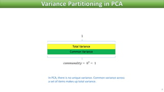
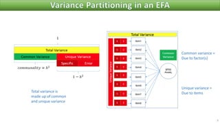
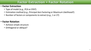
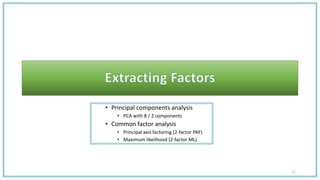
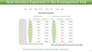
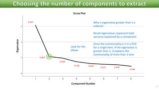
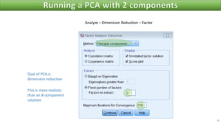
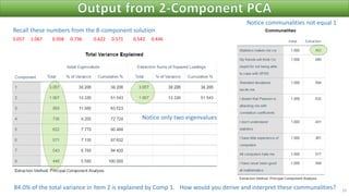
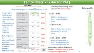
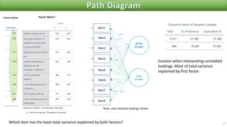
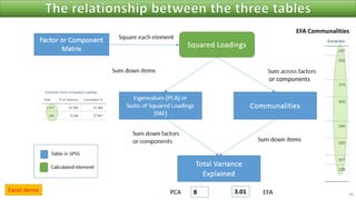
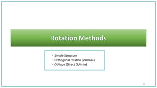
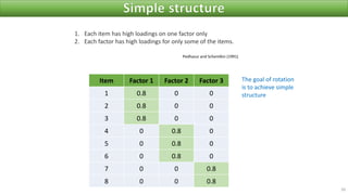
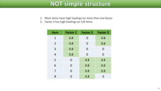
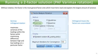
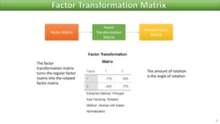
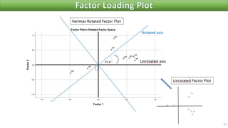
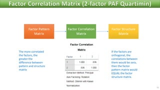
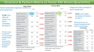
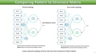
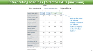
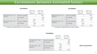
1. IDRE Statistical Consulting
1
https://stats.idre.ucla.edu/spss/seminars/efa-spss/

2. • Introduction
• Motivating example: The SAQ
• Pearson correlation
• Partitioning the variance in factor analysis
• Extracting factors
• Principal components analysis
• Running a PCA with 8 components in SPSS
• Running a PCA with 2 components in SPSS
• Common factor analysis
• Principal axis factoring (2-factor PAF)
• Maximum likelihood (2-factor ML)
• Rotation methods
• Simple Structure
• Orthogonal rotation (Varimax)
• Oblique (Direct Oblimin)
• Generating factor scores
2

3. • Motivating example: The SAQ
• Pearson correlation
• Partitioning the variance in
factor analysis
3

4. 4
Latent variable
Observed variables
Assumption: the correlations among all observed variables can be explained by latent variable

5. 1. I dream that Pearson is attacking me with correlation coefficients
2. I don’t understand statistics
3. I have little experience with computers
4. All computers hate me
5. I have never been good at mathematics
6. My friends are better at statistics than me
7. Computers are useful only for playing games
8. I did badly at mathematics at school
5

6. 6
Large negative Large positive
There exist varying
magnitudes of
correlation among
variables

7. • Common variance
• variance that is shared among a set of items
• Communality (h2)
• common variance that ranges between 0 and 1
• Unique variance
• variance that’s not common
• Specific variance
• variance that is specific to a particular item
• Item 4 “All computers hate me” → anxiety about computers in addition to anxiety about SPSS
• Error variance
• anything unexplained by common or specific variance
• e.g., a mother got a call from her babysitter that her two-year old son ate her favorite lipstick).
7

8. 8
In PCA, there is no unique variance. Common variance across
a set of items makes up total variance.

9. 9
Total variance is
made up of common
and unique variance
Common variance =
Due to factor(s)
Unique variance =
Due to items

10. • Factor Extraction
• Type of model (e.g., PCA or EFA?)
• Estimation method (e.g., Principal Axis Factoring or Maximum Likelihood?)
• Number of factors or components to extract (e.g., 1 or 2?)
• Factor Rotation
• Achieve simple structure
• Orthogonal or oblique?
10

11. • Principal components analysis
• PCA with 8 / 2 components
• Common factor analysis
• Principal axis factoring (2-factor PAF)
• Maximum likelihood (2-factor ML)
11

12. • Principal Components Analysis (PCA)
• Goal: to replicate the correlation matrix using a set of components that are fewer in
number than the original set of items
12
8 variables 2 components
PC1
PC1
Recall communality in PCA

13. • Eigenvalues
• Total variance explained by given principal component
• Eigenvalues > 0, good
• Negative eigenvalues → ill-conditioned
• Eigenvalues close to zero → multicollinearity
• Eigenvectors
• weight for each eigenvalue
• eigenvector times the square root of the eigenvalue → component loadings
• Component loadings
• correlation of each item with the principal component
• Eigenvalues are the sum of squared component loadings across all items for each
component
13

14. Analyze – Dimension Reduction – Factor
14
Note: Factors are NOT the same as Components
8 components is NOT what you typically want to use

15. 15
0.6592 = 0.434
0.1362 = 0.018
43.4% of the variance
explained by first
component (think R-square)
1.8% of the variance
explained by second
component
Sum squared loadings down each
column (component) = eigenvalues
Sum of squared loadings across
components is the communality
3.057 1.067 0.958 0.736 0.622 0.571 0.543 0.446
Q: why is it 1?
Component loadings
correlation of each item with the principal
component
Excel demo
1
1
1
1
1
1
1
1

16. 16
Look familiar? Extraction Sums of Squared Loadings = Eigenvalues
3.057 1.067 0.958 0.736 0.622 0.571 0.543 0.446
Why is the left column the same as the right?

17. 17
3.057
1.067
0.958
0.736 0.622
0.571 0.543
0.446
Look for the
elbow
Why is eigenvalue greater than 1 a
criteria?
Recall eigenvalues represent total
variance explained by a component
Since the communality is 1 in a PCA
for a single item, if the eigenvalue is
greater than 1, it explains the
communality of more than 1 item

18. 18
Analyze – Dimension Reduction – Factor
This is more realistic
than an 8-component
solution
Goal of PCA is
dimension reduction

19. 19
Notice only two eigenvalues
Notice communalities not equal 1
How would you derive and interpret these communalities?
3.057 1.067 0.958 0.736 0.622 0.571 0.543 0.446
Recall these numbers from the 8-component solution
84.0% of the total variance in Item 2 is explained by Comp 1.

20. 20

21. • Principal components analysis
• PCA with 8 / 2 components
• Common factor analysis
• Principal axis factoring (2-factor PAF)
• Maximum likelihood (2-factor ML)
21

22. • Factor Analysis (EFA)
• Goal: also to reduce dimensionality, BUT assume total variance can be divided into
common and unique variance
• Makes more sense to define a construct
with measurement error
22
8 variables
1 variable = factor

23. 23
Analyze – Dimension Reduction – Factor
Make note of the word
eigenvalue it will come
back to haunt us later
SPSS does not change
its menu to reflect
changes in your
analysis. You have to
know the
idiosyncrasies yourself.

24. 24
Initial communalities are
the squared multiple
correlation coefficients
controlling for all other
items in your model
Q: what was the initial
communality for PCA?
Sum of communalities across items = 3.01

25. 25
Unlike the PCA model, the
sum of the initial
eigenvalues do not equal
the sums of squared
loadings
2.510 0.499
Sum eigenvalues = 4.124
The reason is because
Eigenvalues are for PCA
not for factor analysis!
(SPSS idiosyncrasies)
(recall) Sum of communalities across items = 3.01
Sum of squared loadings Factor 1 = 2.51
Sum of squared loadings Factor 2 = 0.499

26. 26
Caution!
Eigenvalues are only for
PCA, yet SPSS uses the
eigenvalue criteria for EFA
When you look at the
scree plot in SPSS, you are
making a conscious
decision to use the PCA
solution as a proxy for
your EFA
Analyze – Dimension Reduction – Factor

27. 27

28. 28
Squaring the
loadings and
summing up
gives you either
the
Communality or
the Extraction
Sums of
Squared
Loadings
Sum of squared loadings across
factors is the communality
Sum squared loadings down each
column = Extraction Sums of Square
Loadings (not eigenvalues)
0.5882 = 0.346
(-0.303)2 = 0.091
34.5% of the variance in
Item 1 explained by first
factor
9.1% of the variance in Item
1 explained by second
factor
0.345 + 0.091 = 0.437
2.510 0.499
0.438
0.052
0.319
0.461
0.344
0.309
0.850
0.236
These are analogous to component loadings in PCA
43.7% of the variance in
Item 1 explained by both
factors = COMMUNALITY!
3.01
Summing down
the
communalities or
across the
eigenvalues gives
you total
variance
explained (3.01)
Communalities

29. 29
Caution when interpreting unrotated
loadings. Most of total variance
explained by first factor.
Communalities
Which item has the least total variance explained by both factors?

30. 30
or components
3.01
EFA Communalities
Excel demo 8
PCA EFA

31. 31

32. 32
New output
A significant chi-
square means you
reject the current
hypothesized model
This is telling us we reject
the two-factor model
Analyze – Dimension Reduction – Factor

33. Number
of Factors
Chi-
square Df p-value
Iterations
needed
1 553.08 20 <0.05 4
2 198.62 13 < 0.05 39
3 13.81 7 0.055 57
4 1.386 2 0.5 168
5 NS -2 NS NS
6 NS -5 NS NS
7 NS -7 NS NS
8 N/A N/A N/A N/A
33
Iterations
needed
goes up
Chi-square and
degrees of freedom
goes down
An eight factor model is not possible in SPSS
The three factor
model is preferred
from chi-square
Want NON-
significant chi-
square

34. 34

35. 35
EFA: Total Variance
Explained = Total
Communality
Explained NOT
Total Variance
PCA: Total Variance
Explained = Total
Variance
For both models,
communality is the
total proportion of
variance due to all
factors or
components in the
model
Communalities are
item specific

36. 36

37. 37
(across all items)

38. • Simple Structure
• Orthogonal rotation (Varimax)
• Oblique (Direct Oblimin)
38

39. Item Factor 1 Factor 2 Factor 3
1 0.8 0 0
2 0.8 0 0
3 0.8 0 0
4 0 0.8 0
5 0 0.8 0
6 0 0.8 0
7 0 0 0.8
8 0 0 0.8
1. Each item has high loadings on one factor only
2. Each factor has high loadings for only some of the items.
39
The goal of rotation
is to achieve simple
structure
Pedhazur and Schemlkin (1991)

40. Item Factor 1 Factor 2 Factor 3
1 0.8 0 0.8
2 0.8 0 0.8
3 0.8 0 0
4 0.8 0 0
5 0 0.8 0.8
6 0 0.8 0.8
7 0 0.8 0.8
8 0 0.8 0
40
1. Most items have high loadings on more than one factor
2. Factor 3 has high loadings on 5/8 items

41. 41
Varimax:
orthogonal rotation
maximizes
variances of the
loadings within the
factors while
maximizing
differences
between high and
low loadings on a
particular factor
Orthogonal means the
factors are uncorrelated
Without rotation, first factor is the most general factor onto which most items load and explains the largest amount of variance

42. 42
The factor
transformation matrix
turns the regular factor
matrix into the rotated
factor matrix
The amount of rotation
is the angle of rotation

43. 43

44. 44
Unrotated solution
maximizes sum of
the variance of
squared loadings
within each factor
0.438
0.052
0.319
0.461
0.344
0.309
0.850
0.236
Varimax rotation
0.437
0.052
0.319
0.461
0.344
0.309
0.850
0.236
communalities are
the same
Communalities Communalities

45. 45
Higher absolute loadings in Varimax solution for Tech Anxiety
Unrotated Solution Varimax Solution

46. 46
3.01 3.01
Even though the distribution of the variance is different the total
sum of squared loadings is the same
maximizes
variances of the
loadings
True or False: Rotation changes how the variances are distributed but not the total communality
Answer: T

47. 47
Varimax: good for distributing among more than one factor
Quartimax: maximizes the squared loadings so that
each item loads most strongly onto a single factor.
Good for generating a single factor.
The difference between Quartimax and
unrotated solution is that maximum
variance can be in a factor that is not the
first

48. • factor pattern matrix
• partial standardized regression coefficients of each item with a particular factor
• Think (P)artial = Pattern
• factor structure matrix
• simple zero order correlations of each item with a particular factor
• Think (S)imple = Structure
• factor correlation matrix
• matrix of intercorrelations among factors
48

49. 49
When Delta =0 →
Direct Quartimin
Oblique rotation
means the factors
are correlated
Larger delta
increases
correlation among
factors
Negative delta
increases makes
factors more
orthogonal

50. 50

51. angle of correlation ϕ
determines whether the factors
are orthogonal or oblique
angle of axis rotation θ
how the axis rotates in relation to
the data points (analogous to
rotation in orthogonal rotation)
51

52. 52
If the factors are
orthogonal, the
correlations between
them would be zero,
then the factor
pattern matrix would
EQUAL the factor
structure matrix.
The more correlated
the factors, the
greater the
difference between
pattern and structure
matrix

53. 53
Simple zero order correlations
(can’t exceed one)
Partial standardized regression coefficients
(can exceed one)
0.653 is the simple
correlation of Factor 1
on Item 1
0.740 is the
effect of
Factor 1 on
Item 1
controlling
for Factor 2
0.566
0.037
0.252
0.436
0.337
0.260
0.871
0.215
0.537
0.082
0.489
0.661
0.489
0.464
1.185
0.344
Note that the sum of
squared loadings do NOT
match communalities
There IS a way
to make the
sum of squared
loadings equal
to the
communality.
Think back to
Orthogonal
Rotation.

54. 54
This is exactly the
same as the
unrotated 2-factor
PAF solution
3.01 4.25
Note: now the sum
of the squared
loadings is HIGHER
than the unrotated
solution
SPSS uses the
structure matrix to
calculate this
-factor contributions
will overlap and
become greater
than the total
variance
SPSS uses the
structure matrix to
calculate this
-factor contributions
will overlap and
become greater
than the total
variance

55. 55
Lower absolute loadings of Items 4,8 onto Tech Anxiety for Pattern Matrix
Partial loadings Zero-order loadings
Correlations same

56. 56
Structure Matrix Pattern Matrix
Why do you think
the second
loading is lower in
the Pattern
Matrix compared
to the Structure
Matrix?

57. • There is no consensus about which one to use in the literature
• Hair et al. (1995)
• Better to interpret the pattern matrix because it gives the unique contribution of the factor
on a particular item
• Pett et al. (2003)
• Structure matrix should be used for interpretation
• Pattern matrix for obtaining factor scores
• My belief: I agree with Hair
Hair, J. F. J., Anderson, R. E., Tatham, R. L., & Black, W. C. (1995). Multivariate data analysis . Saddle River.
Pett, M. A., Lackey, N. R., & Sullivan, J. J. (2003). Making sense of factor analysis: The use of factor analysis for instrument development in health care research. Sage.
57

58. 58

59. • Regression
• Bartlett
• Anderson-Rubin
59

60. 60
Analyze – Dimension Reduction – Factor – Factor Scores
What it looks like in SPSS Data View

61. 61
This is how the factor scores are generated
SPSS takes the standardized scores for each item
Then multiply each score
-0.452
-0.733
1.32
-0.829
-0.749
-0.203
0.0692
-1.42
-0.880
-0.452
-0.733
1.32
-0.829
-0.749
-0.203
0.0692
-1.42
-0.113

62. 62
Covariance matrix of the true factor scores Covariance matrix of the estimated factor scores
Notice that for Direct
Quartimin, the raw
covariances do not match
Regression method has
factor score mean of zero,
and variance equal to the
squared multiple
correlation of estimated
and true factor scores

63. 63
Notice that for Direct Quartimin, the raw
correlations do match (property of
Regression method)
However, note that the factor scores are
still correlated even though we did
Varimax

64. • 1. Regression Method
• Variance equals the square multiple correlation between factors and variables
• Maximizes correlation between estimated and true factor scores but can be biased
• 2. Bartlett
• Factor scores highly correlate with own true factor and not with others
• Unbiased estimate of true factor scores
• 3. Anderson-Rubin
• Estimated factor scores become uncorrelated with other true factors and uncorrelated with
other estimated factor scores
• Biased especially if factors are actually correlated, not for oblique rotations
64

65. 65
Direct Quartimin

66. 66