Download to read offline


![Model
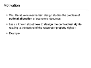
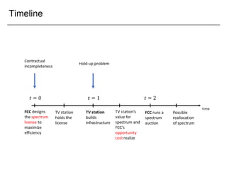
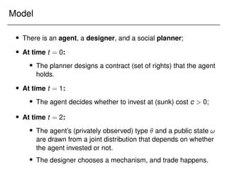
Time t = 2 continued:
Designer chooses a trading mechanism (x!(); t!()), where
x 2 [0; 1] denotes an allocation, and t 2 R denotes a transfer;](https://image.slidesharecdn.com/presentation-231123230350-0f543767/85/Presentation_Yale-pdf-71-320.jpg)
![Model
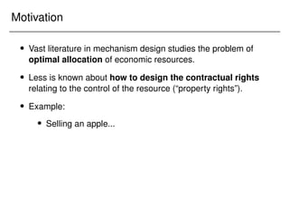
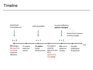
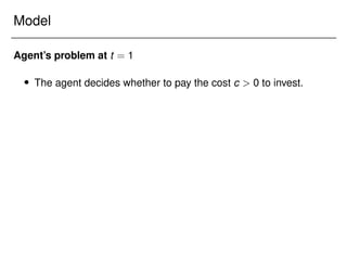
Time t = 2 continued:
Designer chooses a trading mechanism (x!(); t!()), where
x 2 [0; 1] denotes an allocation, and t 2 R denotes a transfer;
Mechanism is chosen subject to IC and IR constraints, and must
respect the rights that the agent holds.](https://image.slidesharecdn.com/presentation-231123230350-0f543767/85/Presentation_Yale-pdf-72-320.jpg)
![Model
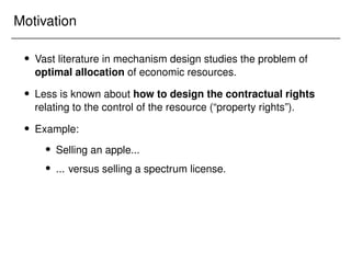
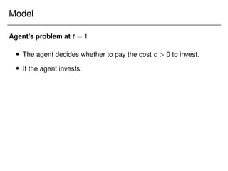
Time t = 2 continued:
Designer chooses a trading mechanism (x!(); t!()), where
x 2 [0; 1] denotes an allocation, and t 2 R denotes a transfer;
Mechanism is chosen subject to IC and IR constraints, and must
respect the rights that the agent holds.
Designer maximizes V(; !) x + t, where 0.](https://image.slidesharecdn.com/presentation-231123230350-0f543767/85/Presentation_Yale-pdf-73-320.jpg)
![Model
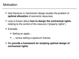
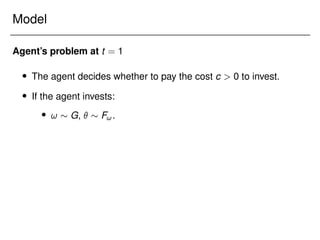
Time t = 2 continued:
Designer chooses a trading mechanism (x!(); t!()), where
x 2 [0; 1] denotes an allocation, and t 2 R denotes a transfer;
Mechanism is chosen subject to IC and IR constraints, and must
respect the rights that the agent holds.
Designer maximizes V(; !) x + t, where 0.
Agent’s utility is x t.](https://image.slidesharecdn.com/presentation-231123230350-0f543767/85/Presentation_Yale-pdf-74-320.jpg)
![Model
Social planner’s problem at t = 0
Social planner chooses a contract that is a menu of “rights”
M = f(xi; ti)gi2I;
where xi 2 [0; 1], ti 2 R, and set I is arbitrary (M is compact).](https://image.slidesharecdn.com/presentation-231123230350-0f543767/85/Presentation_Yale-pdf-82-320.jpg)
![Model
Social planner’s problem at t = 0
Social planner chooses a contract that is a menu of “rights”
M = f(xi; ti)gi2I;
where xi 2 [0; 1], ti 2 R, and set I is arbitrary (M is compact).
The agent can “execute” any one of these rights at t = 2.](https://image.slidesharecdn.com/presentation-231123230350-0f543767/85/Presentation_Yale-pdf-83-320.jpg)
![Model
Social planner’s problem at t = 0
Social planner chooses a contract that is a menu of “rights”
M = f(xi; ti)gi2I;
where xi 2 [0; 1], ti 2 R, and set I is arbitrary (M is compact).
The agent can “execute” any one of these rights at t = 2.
Social planner maximizes V?
(; !)x + ?
t, where ?
0.](https://image.slidesharecdn.com/presentation-231123230350-0f543767/85/Presentation_Yale-pdf-84-320.jpg)
![Model
Social planner’s problem at t = 0
Social planner chooses a contract that is a menu of “rights”
M = f(xi; ti)gi2I;
where xi 2 [0; 1], ti 2 R, and set I is arbitrary (M is compact).
The agent can “execute” any one of these rights at t = 2.
Social planner maximizes V?
(; !)x + ?
t, where ?
0.](https://image.slidesharecdn.com/presentation-231123230350-0f543767/85/Presentation_Yale-pdf-85-320.jpg)
![Model
Social planner’s problem at t = 0
Social planner chooses a contract that is a menu of “rights”
M = f(xi; ti)gi2I;
where xi 2 [0; 1], ti 2 R, and set I is arbitrary (M is compact).
The agent can “execute” any one of these rights at t = 2.
Social planner maximizes V?
(; !)x + ?
t, where ?
0.
Assume: Investment is preferred by the social planner to no
investment; investment can be induced by some contract; but it is not
induced if the agent holds no rights.](https://image.slidesharecdn.com/presentation-231123230350-0f543767/85/Presentation_Yale-pdf-86-320.jpg)
![Model
Social planner’s problem at t = 0
Social planner chooses a contract that is a menu of “rights”
M = f(xi; ti)gi2I;
where xi 2 [0; 1], ti 2 R, and set I is arbitrary (M is compact).
The agent can “execute” any one of these rights at t = 2.
Social planner maximizes V?
(; !)x + ?
t, where ?
0.
Technicalities: Θ [; ¯
] is a compact subset of R; V and V?
are
continuous in (and measurable in !), F has a continuous positive
density on Θ.](https://image.slidesharecdn.com/presentation-231123230350-0f543767/85/Presentation_Yale-pdf-87-320.jpg)
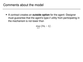
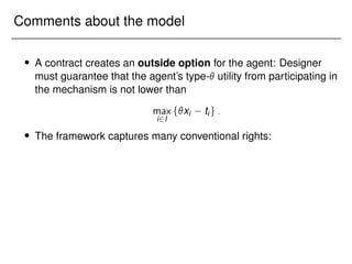
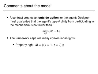
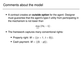
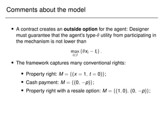
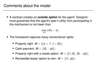
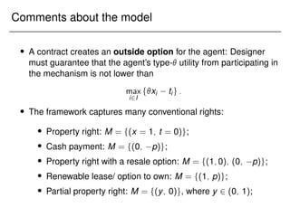
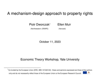
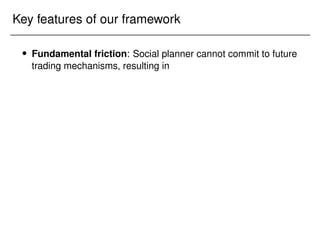
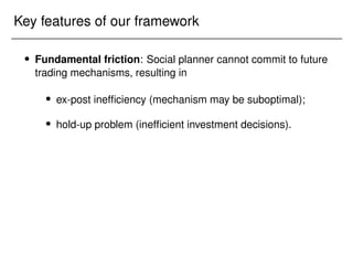
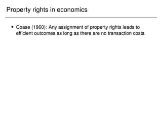
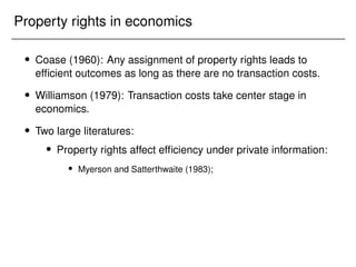
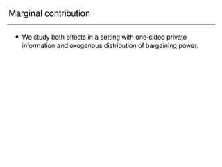
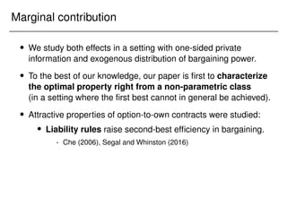
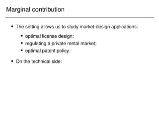
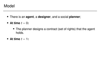
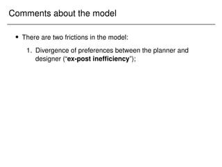
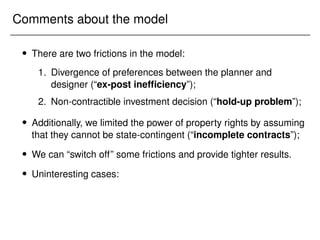
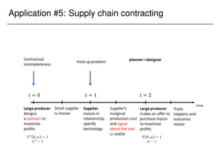
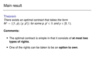
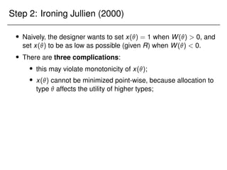
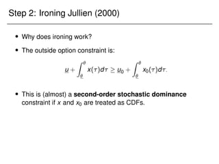
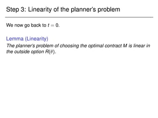
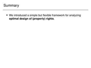
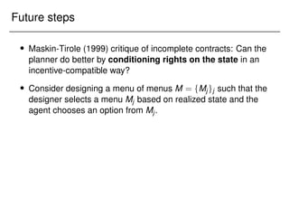
![Comments about the model
A contract creates an outside option for the agent: Designer
must guarantee that the agent’s type- utility from participating in
the mechanism is not lower than
max
i2I
fxi tig:
The framework captures many conventional rights:
Property right: M = f(x = 1; t = 0)g;
Cash payment: M = f(0; p)g;
Property right with a resale option: M = f(1;0); (0; p)g;
Renewable lease/ option to own: M = f(1; p)g;
Partial property right: M = f(y; 0)g, where y 2 (0; 1);
Flexible property right: M = fs; p(s))gs2[0; 1].](https://image.slidesharecdn.com/presentation-231123230350-0f543767/85/Presentation_Yale-pdf-95-320.jpg)
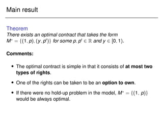
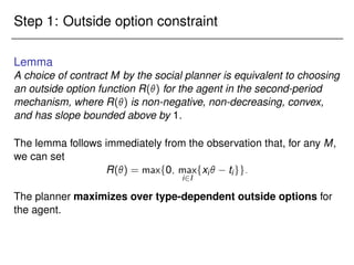
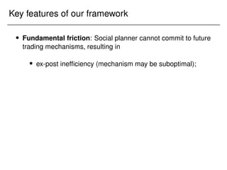
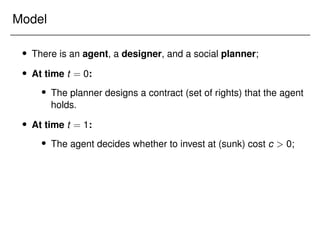
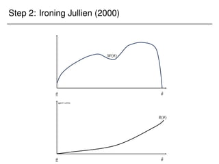
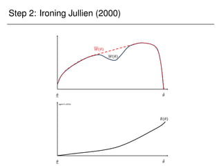
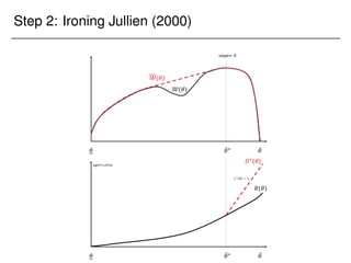
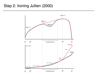
![Step 1: Outside option constraint
Fixing ! (and dropping it from the notation), the designer solves:
max
x:Θ![0;1]; u0
Z
W()x()d u
s.t. x is non-decreasing;
U() u +
Z
x() d R(); 8 2 Θ;
where
W() (V() + B()) f();
and
B() =
1 F()
f()
:](https://image.slidesharecdn.com/presentation-231123230350-0f543767/85/Presentation_Yale-pdf-118-320.jpg)
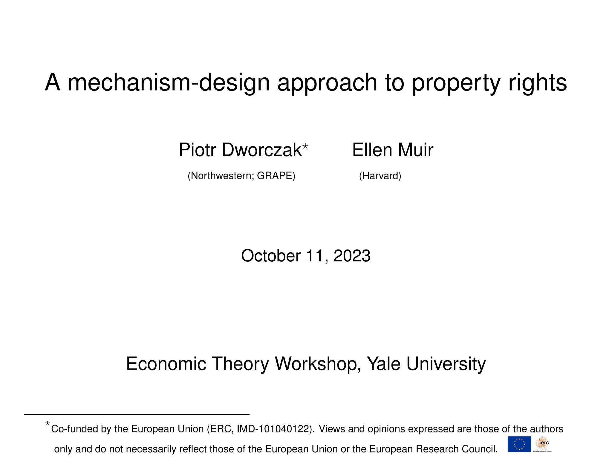
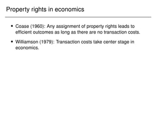
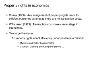
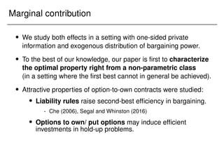
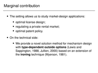
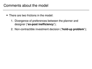
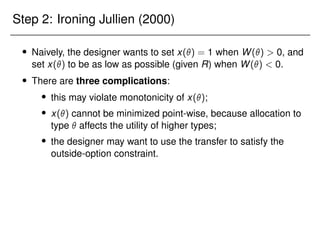
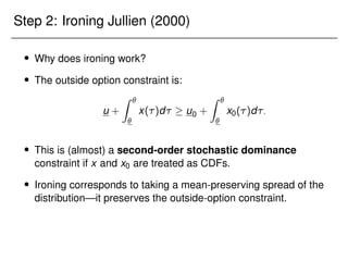
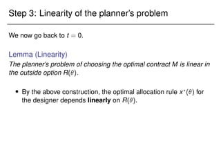
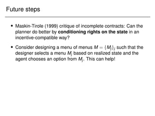
![Step 1: Outside option constraint
Fixing ! (and dropping it from the notation), the designer solves:
max
x:Θ![0;1]; u0
Z
W()x()d u
s.t. x is non-decreasing;
U() u +
Z
x() d R(); 8 2 Θ;
where
W() (V() + B()) f();
and
B() =
1 F()
f()
:
This is a problem considered by Jullien (2000).](https://image.slidesharecdn.com/presentation-231123230350-0f543767/85/Presentation_Yale-pdf-119-320.jpg)

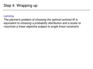
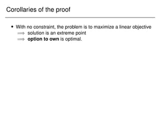
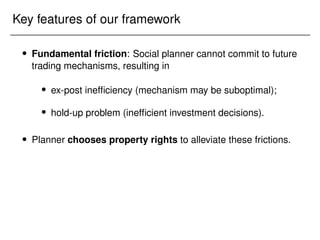
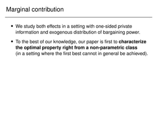
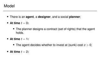
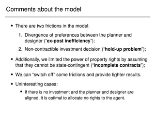
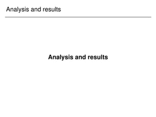
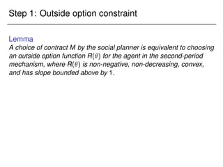
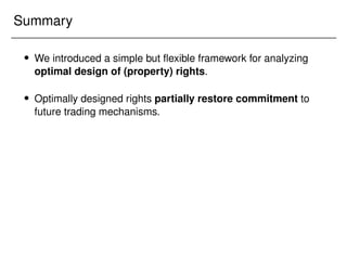
![Corollaries of the proof
With no constraint, the problem is to maximize a linear objective
=) solution is an extreme point
=) option to own is optimal.
Easy extension to K linear constraints
=) We need at most K + 1 options in the optimal menu.
Extension to continuous investment:
Suppose agent chooses e 2 [0; 1] at strictly convex cost
c(e), and e is the probability that is drawn from F!.](https://image.slidesharecdn.com/presentation-231123230350-0f543767/85/Presentation_Yale-pdf-151-320.jpg)
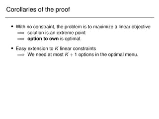
![Corollaries of the proof
With no constraint, the problem is to maximize a linear objective
=) solution is an extreme point
=) option to own is optimal.
Easy extension to K linear constraints
=) We need at most K + 1 options in the optimal menu.
Extension to continuous investment:
Suppose agent chooses e 2 [0; 1] at strictly convex cost
c(e), and e is the probability that is drawn from F!.
Satisfying FOC at the target investment level e?
is sufficient
for obedience.](https://image.slidesharecdn.com/presentation-231123230350-0f543767/85/Presentation_Yale-pdf-152-320.jpg)
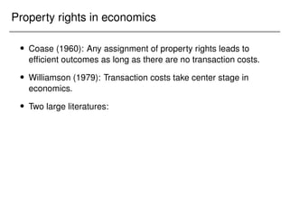
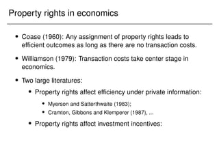
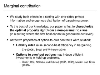
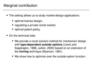
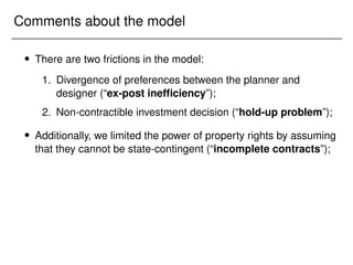
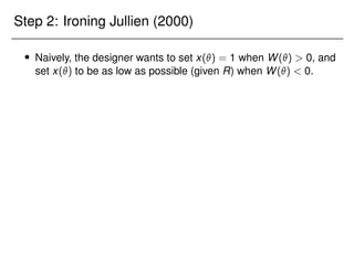
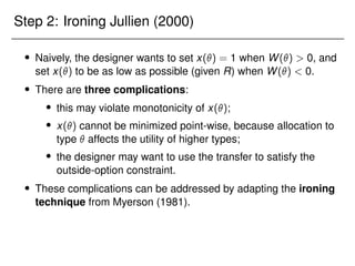
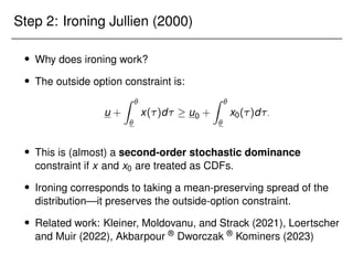
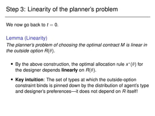
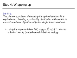
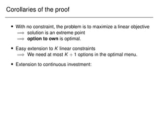
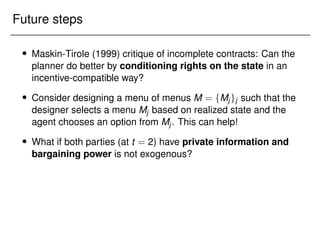
![Corollaries of the proof
With no constraint, the problem is to maximize a linear objective
=) solution is an extreme point
=) option to own is optimal.
Easy extension to K linear constraints
=) We need at most K + 1 options in the optimal menu.
Extension to continuous investment:
Suppose agent chooses e 2 [0; 1] at strictly convex cost
c(e), and e is the probability that is drawn from F!.
Satisfying FOC at the target investment level e?
is sufficient
for obedience.
FOC is linear in R() =) we need two options in the
optimal menu.](https://image.slidesharecdn.com/presentation-231123230350-0f543767/85/Presentation_Yale-pdf-153-320.jpg)
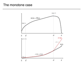
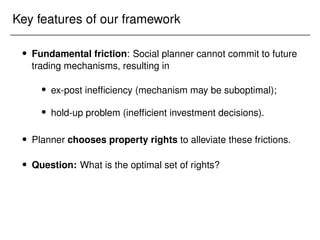
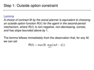
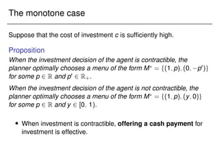
![The monotone case
Lemma (The monotone case)
For any outside option function R(), the mechanism designer in the
second period will choose an optimal mechanism in which the
outside-option constraint binds for types in the interval [?
!; ¯
?
!].](https://image.slidesharecdn.com/presentation-231123230350-0f543767/85/Presentation_Yale-pdf-156-320.jpg)
![The monotone case
Lemma (The monotone case)
For any outside option function R(), the mechanism designer in the
second period will choose an optimal mechanism in which the
outside-option constraint binds for types in the interval [?
!; ¯
?
!].
Moreover, except for the case of a boundary solution,
V(?
!; !) + S(?
!) = 0;
V(¯
?
!; !) + B(¯
?
!) = 0:](https://image.slidesharecdn.com/presentation-231123230350-0f543767/85/Presentation_Yale-pdf-157-320.jpg)
![The monotone case
Lemma (The monotone case)
For any outside option function R(), the mechanism designer in the
second period will choose an optimal mechanism in which the
outside-option constraint binds for types in the interval [?
!; ¯
?
!].
Moreover, except for the case of a boundary solution,
V(?
!; !) + S(?
!) = 0;
V(¯
?
!; !) + B(¯
?
!) = 0:
For ¯
?
!, the designer wants to allocate the good to the agent
anyway, so the outside-option constraint is slack;](https://image.slidesharecdn.com/presentation-231123230350-0f543767/85/Presentation_Yale-pdf-158-320.jpg)
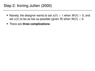
![The monotone case
Lemma (The monotone case)
For any outside option function R(), the mechanism designer in the
second period will choose an optimal mechanism in which the
outside-option constraint binds for types in the interval [?
!; ¯
?
!].
Moreover, except for the case of a boundary solution,
V(?
!; !) + S(?
!) = 0;
V(¯
?
!; !) + B(¯
?
!) = 0:
For ¯
?
!, the designer wants to allocate the good to the agent
anyway, so the outside-option constraint is slack;](https://image.slidesharecdn.com/presentation-231123230350-0f543767/85/Presentation_Yale-pdf-159-320.jpg)
![The monotone case
Lemma (The monotone case)
For any outside option function R(), the mechanism designer in the
second period will choose an optimal mechanism in which the
outside-option constraint binds for types in the interval [?
!; ¯
?
!].
Moreover, except for the case of a boundary solution,
V(?
!; !) + S(?
!) = 0;
V(¯
?
!; !) + B(¯
?
!) = 0:
For ¯
?
!, the designer wants to allocate the good to the agent
anyway, so the outside-option constraint is slack;
For ?
!, the designer prefers to “buy out” the rights using a
monetary payment, so the constraint is again slack.](https://image.slidesharecdn.com/presentation-231123230350-0f543767/85/Presentation_Yale-pdf-160-320.jpg)
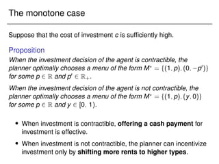
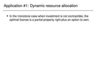
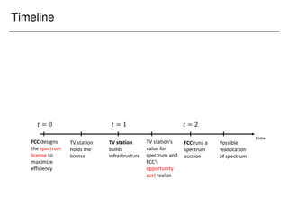
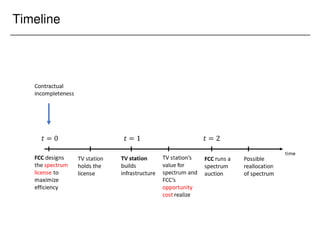
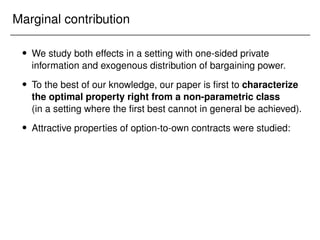
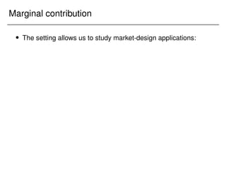
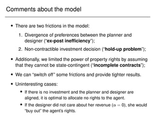
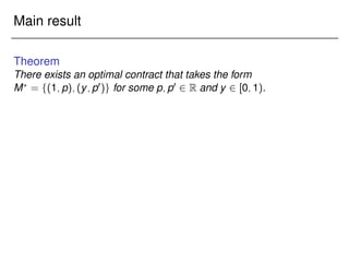
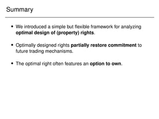
![Application #1: Dynamic resource allocation
In the monotone case when investment is not contractible, the
optimal license is a partial property right plus an option to own.
Suppose that F! is uniform on [0; 1], and F! is an atom at 0.](https://image.slidesharecdn.com/presentation-231123230350-0f543767/85/Presentation_Yale-pdf-169-320.jpg)
![Application #1: Dynamic resource allocation
In the monotone case when investment is not contractible, the
optimal license is a partial property right plus an option to own.
Suppose that F! is uniform on [0; 1], and F! is an atom at 0.
The optimal property right as a function of value for revenue:](https://image.slidesharecdn.com/presentation-231123230350-0f543767/85/Presentation_Yale-pdf-170-320.jpg)
![Application #1: Dynamic resource allocation
In the monotone case when investment is not contractible, the
optimal license is a partial property right plus an option to own.
Suppose that F! is uniform on [0; 1], and F! is an atom at 0.
The optimal property right as a function of value for revenue:
= ?
= 1: option to own (1; p)
(p makes the investment-obedience constraint bind);](https://image.slidesharecdn.com/presentation-231123230350-0f543767/85/Presentation_Yale-pdf-171-320.jpg)
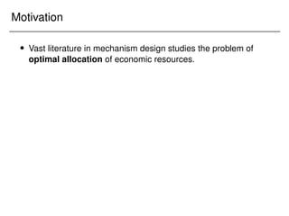
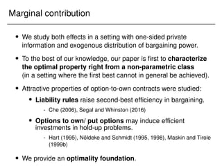
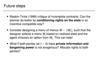
![Application #1: Dynamic resource allocation
In the monotone case when investment is not contractible, the
optimal license is a partial property right plus an option to own.
Suppose that F! is uniform on [0; 1], and F! is an atom at 0.
The optimal property right as a function of value for revenue:
= ?
= 1: option to own (1; p)
(p makes the investment-obedience constraint bind);
= 1; ?
= 0: partial property right (0; y)
(y makes the investment-obedience constraint bind);](https://image.slidesharecdn.com/presentation-231123230350-0f543767/85/Presentation_Yale-pdf-172-320.jpg)
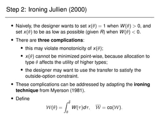
![Application #1: Dynamic resource allocation
In the monotone case when investment is not contractible, the
optimal license is a partial property right plus an option to own.
Suppose that F! is uniform on [0; 1], and F! is an atom at 0.
The optimal property right as a function of value for revenue:
= ?
= 1: option to own (1; p)
(p makes the investment-obedience constraint bind);
= 1; ?
= 0: partial property right (0; y)
(y makes the investment-obedience constraint bind);
= ?
= 0: no right
(consistent with Rogerson (1992))](https://image.slidesharecdn.com/presentation-231123230350-0f543767/85/Presentation_Yale-pdf-173-320.jpg)
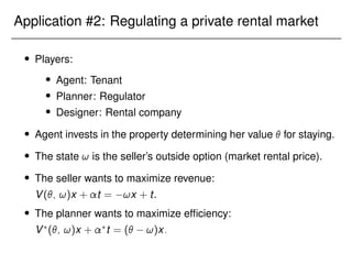
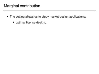
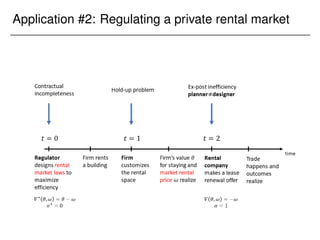
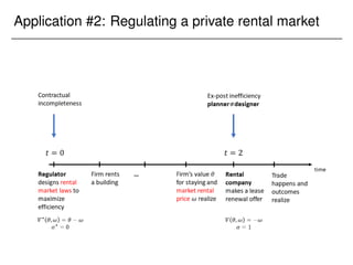
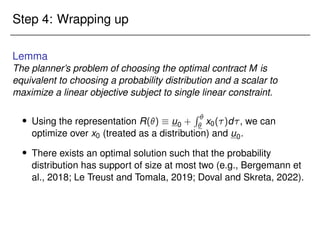
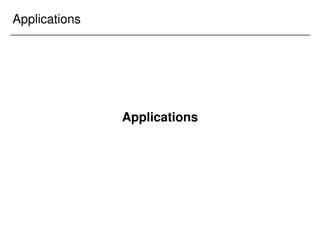
![Application #2: Regulating a private rental market
Suppose that without investment, value is uniform on [0; 1];
with investment, the value is drawn from [∆; 1 + ∆] instead.](https://image.slidesharecdn.com/presentation-231123230350-0f543767/85/Presentation_Yale-pdf-175-320.jpg)
![Application #2: Regulating a private rental market
Suppose that without investment, value is uniform on [0; 1];
with investment, the value is drawn from [∆; 1 + ∆] instead.
Suppose that ! is known (and lies in a certain range).](https://image.slidesharecdn.com/presentation-231123230350-0f543767/85/Presentation_Yale-pdf-176-320.jpg)
![Application #2: Regulating a private rental market
Suppose that without investment, value is uniform on [0; 1];
with investment, the value is drawn from [∆; 1 + ∆] instead.
Suppose that ! is known (and lies in a certain range).
The optimal contract is a renewable lease with price
p?
= ! ∆;
where is the Lagrange multiplier on the investment constraint.](https://image.slidesharecdn.com/presentation-231123230350-0f543767/85/Presentation_Yale-pdf-177-320.jpg)
![Application #2: Regulating a private rental market
Suppose that without investment, value is uniform on [0; 1];
with investment, the value is drawn from [∆; 1 + ∆] instead.
Suppose that ! is known (and lies in a certain range).
The optimal contract is a renewable lease with price
p?
= ! ∆;
where is the Lagrange multiplier on the investment constraint.
If investment constraint is slack, p?
= !, so the planner “forces”
the seller to use a VCG mechanism.](https://image.slidesharecdn.com/presentation-231123230350-0f543767/85/Presentation_Yale-pdf-178-320.jpg)
![Application #2: Regulating a private rental market
Suppose that without investment, value is uniform on [0; 1];
with investment, the value is drawn from [∆; 1 + ∆] instead.
Suppose that ! is known (and lies in a certain range).
The optimal contract is a renewable lease with price
p?
= ! ∆;
where is the Lagrange multiplier on the investment constraint.
If investment constraint is slack, p?
= !, so the planner “forces”
the seller to use a VCG mechanism.
If ! is random, then (assuming interior solution)
p?
= E[ ! j ?
! p?
?
!] ∆:](https://image.slidesharecdn.com/presentation-231123230350-0f543767/85/Presentation_Yale-pdf-179-320.jpg)
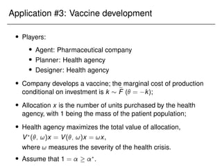
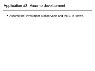
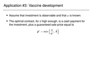
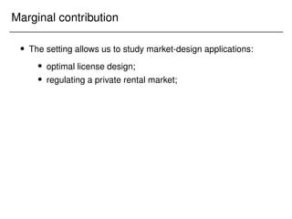
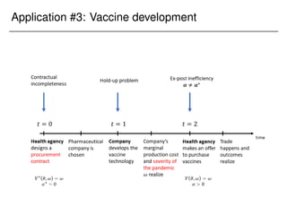
![Application #3: Vaccine development
If ! is stochastic, then the optimal price satisfies
p?
= min
(
E
!j! 2 [!p? ; ¯
!p? ]
?
; k̄
)
;
where [!p? ; ¯
!p? ] is the interval of !’s for which the choice of p?
changes the second-period mechanism.](https://image.slidesharecdn.com/presentation-231123230350-0f543767/85/Presentation_Yale-pdf-185-320.jpg)
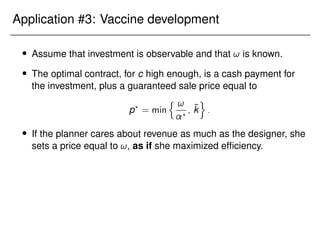
![Application #3: Vaccine development
If ! is stochastic, then the optimal price satisfies
p?
= min
(
E
!j! 2 [!p? ; ¯
!p? ]
?
; k̄
)
;
where [!p? ; ¯
!p? ] is the interval of !’s for which the choice of p?
changes the second-period mechanism.
If the realized ! is high (health crisis is severe), the designer will
offer a price better than p?
.](https://image.slidesharecdn.com/presentation-231123230350-0f543767/85/Presentation_Yale-pdf-186-320.jpg)
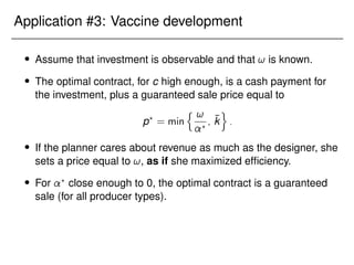
![Application #3: Vaccine development
If ! is stochastic, then the optimal price satisfies
p?
= min
(
E
!j! 2 [!p? ; ¯
!p? ]
?
; k̄
)
;
where [!p? ; ¯
!p? ] is the interval of !’s for which the choice of p?
changes the second-period mechanism.
If the realized ! is high (health crisis is severe), the designer will
offer a price better than p?
.
If the realized ! is low (health crisis is mild), the designer will
offer a price lower than p?
and compensate the producer with an
additional cash payment (on top of the payment for investment).](https://image.slidesharecdn.com/presentation-231123230350-0f543767/85/Presentation_Yale-pdf-187-320.jpg)
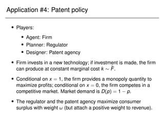
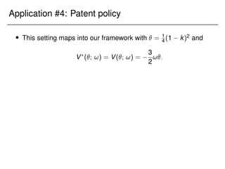
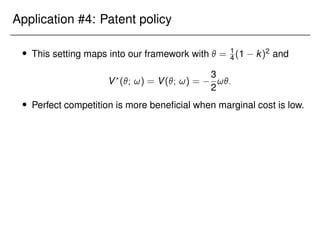
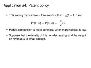
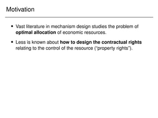
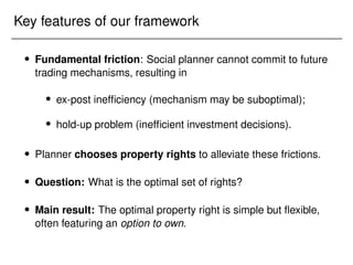
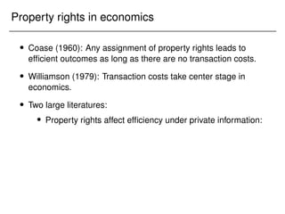
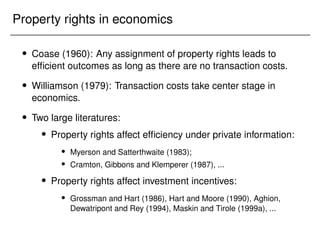
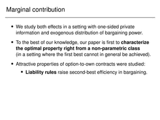
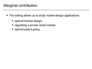
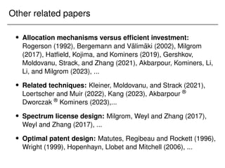
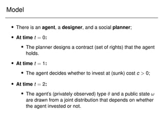
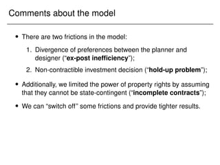
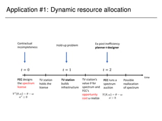
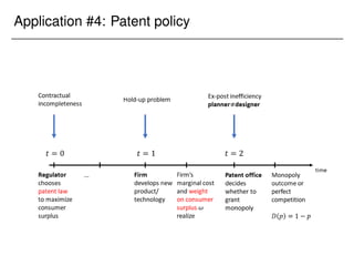
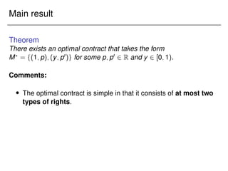
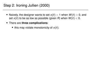
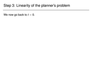
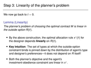
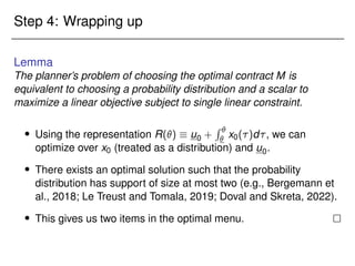
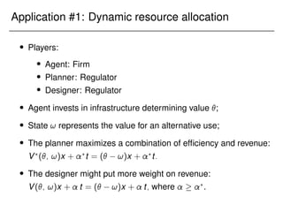
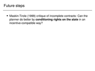
![Application #4: Patent policy
This setting maps into our framework with = 1
4 (1 k)2 and
V?
(; !) = V(; !) =
3
2
!:
Perfect competition is more beneficial when marginal cost is low.
Suppose that the density of is non-decreasing, and the weight
on revenue is small enough.
Then, an optimal contract is to offer full patent protection to the
invention (x = 1) with exogenous probability y 2 (0; 1] at no
payment.](https://image.slidesharecdn.com/presentation-231123230350-0f543767/85/Presentation_Yale-pdf-192-320.jpg)

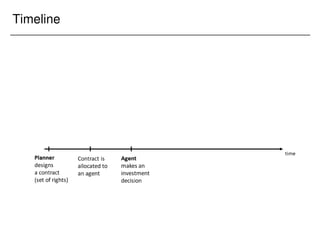
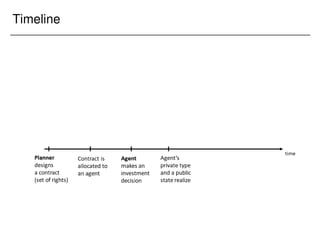
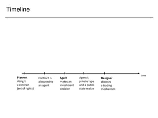
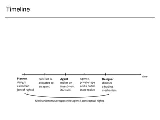
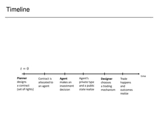
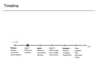
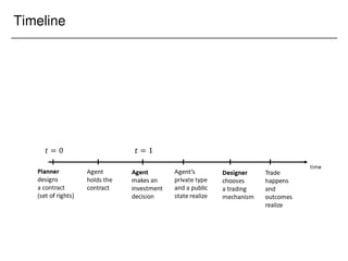
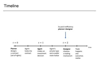
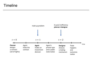
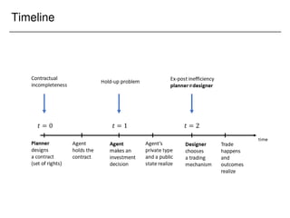
The document presents a framework for studying the optimal design of contractual property rights using mechanism design. It discusses how property rights determine agents' outside options in economic interactions and impact ex-post efficiency and investment incentives when the social planner cannot commit to future mechanisms. The authors analyze how to design property rights to alleviate these frictions in a setting with one-sided private information and bargaining power. A key result is that the optimal property right is often simple but flexible, featuring an option to own the resource.


