A mechanism-design approach to property rights
Piotr Dworczak?
Ellen Muir
(Northwestern; GRAPE) (Harvard)
October 9, 2023
Economic Theory Workshop, Columbia University
?
Co-funded by the European Union (ERC, IMD-101040122). Views and opinions expressed are those of the authors
only and do not necessarily reflect those of the European Union or the European Research Council.
Motivation
 Vast literature in mechanism design studies the problem of
optimal allocation of economic resources.
Motivation
 Vast literature in mechanism design studies the problem of
optimal allocation of economic resources.
 Less is known about how to design the contractual rights
relating to the control of the resource (“property rights”).
Motivation
 Vast literature in mechanism design studies the problem of
optimal allocation of economic resources.
 Less is known about how to design the contractual rights
relating to the control of the resource (“property rights”).
 Example:
Motivation
 Vast literature in mechanism design studies the problem of
optimal allocation of economic resources.
 Less is known about how to design the contractual rights
relating to the control of the resource (“property rights”).
 Example:
 Selling an apple...
Motivation
 Vast literature in mechanism design studies the problem of
optimal allocation of economic resources.
 Less is known about how to design the contractual rights
relating to the control of the resource (“property rights”).
 Example:
 Selling an apple...
 ... versus selling a spectrum license.
 We provide a framework for studying optimal design of
contractual rights.
Key features of our framework
 In our framework, property rights determine the holder’s
outside options (with regard to the underlying good) in
economic interactions:
Key features of our framework
 In our framework, property rights determine the holder’s
outside options (with regard to the underlying good) in
economic interactions:
 Full property right: Holder can always keep the good;
Key features of our framework
 In our framework, property rights determine the holder’s
outside options (with regard to the underlying good) in
economic interactions:
 Full property right: Holder can always keep the good;
 No rights: Outside option is (normalized to) zero;
Key features of our framework
 In our framework, property rights determine the holder’s
outside options (with regard to the underlying good) in
economic interactions:
 Full property right: Holder can always keep the good;
 No rights: Outside option is (normalized to) zero;
 Renewable lease: Holder can keep the good at a price;
 ...
 We model the economic interaction as the holder of the rights
participating in a trading mechanism.
Key features of our framework
 Fundamental friction: Social planner cannot commit to future
trading mechanisms, resulting in
Key features of our framework
 Fundamental friction: Social planner cannot commit to future
trading mechanisms, resulting in
 ex-post inefficiency (mechanism may be suboptimal);
Key features of our framework
 Fundamental friction: Social planner cannot commit to future
trading mechanisms, resulting in
 ex-post inefficiency (mechanism may be suboptimal);
 hold-up problem (inefficient investment decisions).
Key features of our framework
 Fundamental friction: Social planner cannot commit to future
trading mechanisms, resulting in
 ex-post inefficiency (mechanism may be suboptimal);
 hold-up problem (inefficient investment decisions).
 Planner chooses property rights to alleviate these frictions.
Key features of our framework
 Fundamental friction: Social planner cannot commit to future
trading mechanisms, resulting in
 ex-post inefficiency (mechanism may be suboptimal);
 hold-up problem (inefficient investment decisions).
 Planner chooses property rights to alleviate these frictions.
 Question: What is the optimal set of rights?
 Main result: The optimal property right is simple but flexible,
often featuring an option to own.
Property rights in economics
 Coase (1960): Any assignment of property rights leads to
efficient outcomes as long as there are transaction costs.
Property rights in economics
 Coase (1960): Any assignment of property rights leads to
efficient outcomes as long as there are transaction costs.
 Williamson (1979): Transaction costs take center stage in
economics.
Property rights in economics
 Coase (1960): Any assignment of property rights leads to
efficient outcomes as long as there are transaction costs.
 Williamson (1979): Transaction costs take center stage in
economics.
 Two large literatures:
Property rights in economics
 Coase (1960): Any assignment of property rights leads to
efficient outcomes as long as there are transaction costs.
 Williamson (1979): Transaction costs take center stage in
economics.
 Two large literatures:
 Property rights affect efficiency under private information:
 Myerson and Satterthwaite (1983);
 Cramton, Gibbons and Klemperer (1987), ...
 Property rights affect investment incentives:
 Grossman and Hart (1986), Hart and Moore (1990), Aghion,
Dewatripont and Rey (1994), Maskin and Tirole (1999), ...
Marginal contribution
 We study both effects in a setting with one-sided private
information and exogenous distribution of bargaining power.
Marginal contribution
 We study both effects in a setting with one-sided private
information and exogenous distribution of bargaining power.
 To the best of our knowledge, our paper is first to characterize
the optimal property right from a non-parametric class
(in a setting where the first best cannot in general be achieved).
 Attractive properties of option-to-own contracts were studied:
 Liability rules raise second-best efficiency in bargaining.
- Che (2006), Segal and Whinston (2016)
 Options to own may induce efficient investments.
- Hart (1995), Nöldeke and Schmidt (1995, 1998)
 We provide an optimality foundation.
Marginal contribution
 The setting allows us to study market-design applications:
Marginal contribution
 The setting allows us to study market-design applications:
 optimal license design;
Marginal contribution
 The setting allows us to study market-design applications:
 optimal license design;
 regulating a private rental market;
Marginal contribution
 The setting allows us to study market-design applications:
 optimal license design;
 regulating a private rental market;
 optimal patent policy.
Marginal contribution
 The setting allows us to study market-design applications:
 optimal license design;
 regulating a private rental market;
 optimal patent policy.
 On the technical side:
Marginal contribution
 The setting allows us to study market-design applications:
 optimal license design;
 regulating a private rental market;
 optimal patent policy.
 On the technical side:
 We provide a novel solution method for mechanism design
with type-dependent outside options (Lewis and
Sappington, 1988, Jullien, 2000) based on an extension of
the ironing technique (Myerson, 1981).
 We show how to optimize over the outside-option function.
Other related papers
 Allocation mechanisms versus efficient investment:
Rogerson (1992), Bergemann and Välimäki (2002), Milgrom
(2017), Hatfield, Kojima, and Kominers (2019), Akbarpour,
Kominers, Li, Li, and Milgrom (2023), ...
 Related techniques: Kleiner, Moldovanu, and Strack (2021),
Loertscher and Muir (2022), Kang (2023), Akbarpour ®
Dworczak ® Kominers (2023),...
 Spectrum license design: Milgrom, Weyl and Zhang (2017),
Weyl and Zhang (2017), ...
 Optimal patent design: Matutes, Regibeau and Rockett (1996),
Wright (1999), Hopenhayn, Llobet and Mitchell (2006), ...
Model
Model
Model
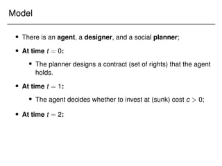
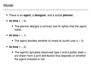
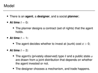
 There is an agent, a designer, and a social planner;
Model
 There is an agent, a designer, and a social planner;
 At time t = 0:
Model
 There is an agent, a designer, and a social planner;
 At time t = 0:
 The planner designs a contract (set of rights) that the agent
holds.
Model
 There is an agent, a designer, and a social planner;
 At time t = 0:
 The planner designs a contract (set of rights) that the agent
holds.
 At time t = 1:
Model
 There is an agent, a designer, and a social planner;
 At time t = 0:
 The planner designs a contract (set of rights) that the agent
holds.
 At time t = 1:
 The agent decides whether to invest at (sunk) cost c  0;
Model
 There is an agent, a designer, and a social planner;
 At time t = 0:
 The planner designs a contract (set of rights) that the agent
holds.
 At time t = 1:
 The agent decides whether to invest at (sunk) cost c  0;
 At time t = 2:
Model
 There is an agent, a designer, and a social planner;
 At time t = 0:
 The planner designs a contract (set of rights) that the agent
holds.
 At time t = 1:
 The agent decides whether to invest at (sunk) cost c  0;
 At time t = 2:
 The agent’s (privately observed) type  and a public state !
are drawn from a joint distribution that depends on whether
the agent invested or not.
 The designer chooses a mechanism, and trade happens.
Model
Time t = 2 continued:
 Designer chooses a trading mechanism (x!(); t!()), where
x 2 [0; 1] denotes an allocation, and t 2 R denotes a transfer;
Model
Time t = 2 continued:
 Designer chooses a trading mechanism (x!(); t!()), where
x 2 [0; 1] denotes an allocation, and t 2 R denotes a transfer;
 Mechanism is chosen subject to IC and IR constraints, and must
respect the rights that the agent holds.
Model
Time t = 2 continued:
 Designer chooses a trading mechanism (x!(); t!()), where
x 2 [0; 1] denotes an allocation, and t 2 R denotes a transfer;
 Mechanism is chosen subject to IC and IR constraints, and must
respect the rights that the agent holds.
 Designer maximizes V(; !) x + t, where  0.
Model
Time t = 2 continued:
 Designer chooses a trading mechanism (x!(); t!()), where
x 2 [0; 1] denotes an allocation, and t 2 R denotes a transfer;
 Mechanism is chosen subject to IC and IR constraints, and must
respect the rights that the agent holds.
 Designer maximizes V(; !) x + t, where  0.
 Agent’s utility is  x t.
Model
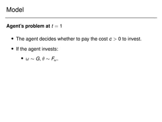
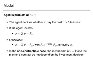
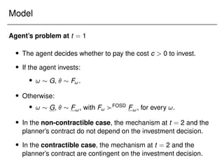
Agent’s problem at t = 1
 The agent decides whether to pay the cost c  0 to invest.
Model
Agent’s problem at t = 1
 The agent decides whether to pay the cost c  0 to invest.
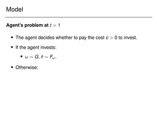
 If the agent invests:
Model
Agent’s problem at t = 1
 The agent decides whether to pay the cost c  0 to invest.
 If the agent invests:
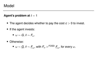
 !  G,   F!.
Model
Agent’s problem at t = 1
 The agent decides whether to pay the cost c  0 to invest.
 If the agent invests:
 !  G,   F!.
 Otherwise:
Model
Agent’s problem at t = 1
 The agent decides whether to pay the cost c  0 to invest.
 If the agent invests:
 !  G,   F!.
 Otherwise:
 !  G,   F!, with F! FOSD F!, for every !.
Model
Agent’s problem at t = 1
 The agent decides whether to pay the cost c  0 to invest.
 If the agent invests:
 !  G,   F!.
 Otherwise:
 !  G,   F!, with F! FOSD F!, for every !.
 In the non-contractible case, the mechanism at t = 2 and the
planner’s contract do not depend on the investment decision.
 In the contractible case, the mechanism at t = 2 and the
planner’s contract are contingent on the investment decision.
Model
Social planner’s problem at t = 0
 Social planner chooses a contract that is a menu of “rights”
M = f(xi; ti)gi2I;
where xi 2 [0; 1], ti 2 R, and set I is arbitrary (M is compact).
Model
Social planner’s problem at t = 0
 Social planner chooses a contract that is a menu of “rights”
M = f(xi; ti)gi2I;
where xi 2 [0; 1], ti 2 R, and set I is arbitrary (M is compact).
 The agent can “execute” any one of these rights at t = 2.
Model
Social planner’s problem at t = 0
 Social planner chooses a contract that is a menu of “rights”
M = f(xi; ti)gi2I;
where xi 2 [0; 1], ti 2 R, and set I is arbitrary (M is compact).
 The agent can “execute” any one of these rights at t = 2.
 Social planner maximizes V?
(; !)x + ?
t, where ?
 0.
Assume: Investment is preferred by the social planner to no
investment; investment can be induced by some contract; but it is not
induced if the agent holds no rights.
Model
Social planner’s problem at t = 0
 Social planner chooses a contract that is a menu of “rights”
M = f(xi; ti)gi2I;
where xi 2 [0; 1], ti 2 R, and set I is arbitrary (M is compact).
 The agent can “execute” any one of these rights at t = 2.
 Social planner maximizes V?
(; !)x + ?
t, where ?
 0.
Technicalities: Θ  [; ¯
] is a compact subset of R; V and V?
are
continuous in  (and measurable in !), F has a continuous positive
density on Θ.
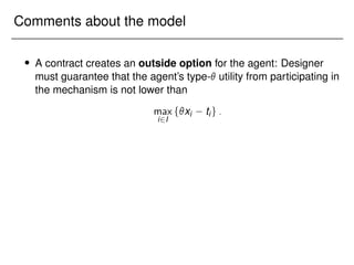
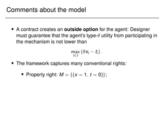
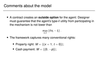
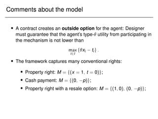
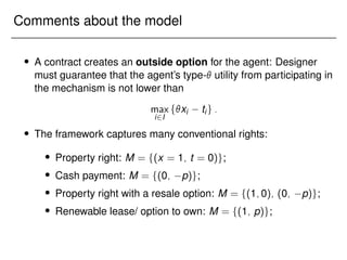
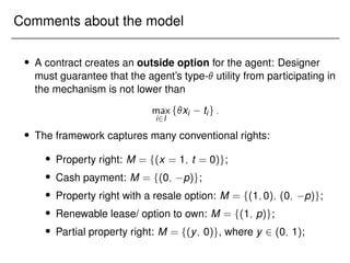
Comments about the model
 A contract creates an outside option for the agent: Designer
must guarantee that the agent’s type- utility from participating in
the mechanism is not lower than
max
i2I
fxi tig:
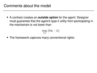
Comments about the model
 A contract creates an outside option for the agent: Designer
must guarantee that the agent’s type- utility from participating in
the mechanism is not lower than
max
i2I
fxi tig:
 The framework captures many conventional rights:
Comments about the model
 A contract creates an outside option for the agent: Designer
must guarantee that the agent’s type- utility from participating in
the mechanism is not lower than
max
i2I
fxi tig:
 The framework captures many conventional rights:
 Property right: M = f(x = 1; t = 0)g;
Comments about the model
 A contract creates an outside option for the agent: Designer
must guarantee that the agent’s type- utility from participating in
the mechanism is not lower than
max
i2I
fxi tig:
 The framework captures many conventional rights:
 Property right: M = f(x = 1; t = 0)g;
 Cash payment: M = f(0; p)g;
 Property right with a resale option: M = f(1;0); (0; p)g;
 Renewable lease/ option to own: M = f(1; p)g;
 Partial property right: M = f(y; 0)g, where y 2 (0; 1);
 Flexible property right: M = fs; p(s))gs2[0; 1].
Comments about the model
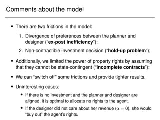
 There are two frictions in the model:
Comments about the model
 There are two frictions in the model:
1. Divergence of preferences between the planner and
designer (“ex-post inefficiency”);
Comments about the model
 There are two frictions in the model:
1. Divergence of preferences between the planner and
designer (“ex-post inefficiency”);
2. Non-contractible investment decision (“hold-up problem”);
Comments about the model
 There are two frictions in the model:
1. Divergence of preferences between the planner and
designer (“ex-post inefficiency”);
2. Non-contractible investment decision (“hold-up problem”);
 Additionally, we limited the power of property rights by assuming
that they cannot be state-contingent (“incomplete contracts”);
 We can “switch off” some frictions and provide tighter results.
 Uninteresting cases:
 If there is no investment and the planner and designer are
aligned, it is optimal to allocate no rights to the agent.
 If the designer did not care about her revenue ( = 0), she would
“buy out” the agent’s rights.
Application #1: Dynamic resource allocation
 Players:
 Agent: Firm
 Planner: Regulator
 Designer: Regulator
 Agent invests in infrastructure determining value ;
 State ! represents the value for an alternative use;
 The planner maximizes a combination of efficiency and revenue:
V?
(; !)x + ?
t = ( !)x + ?
t:
 The designer might put more weight on revenue:
V(; !)x + t = ( !)x + t; where  ?
.
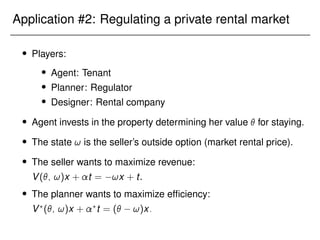
Application #2: Regulating a private rental market
 Players:
 Agent: Tenant
 Planner: Regulator
 Designer: Rental company
 Agent invests in the property determining her value  for staying.
 The state ! is the seller’s outside option (market rental price).
 The seller wants to maximize revenue:
V(; !)x + t = !x + t.
 The planner wants to maximize efficiency:
V?
(; !)x + ?
t = ( !)x:
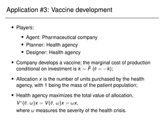
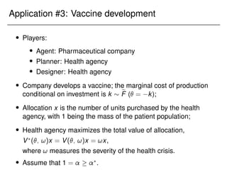
Application #3: Vaccine development
 Players:
 Agent: Pharmaceutical company
 Planner: Health agency
 Designer: Health agency
 Company develops a vaccine; the marginal cost of production
conditional on investment is k  F̃ ( = k);
 Allocation x is the number of units purchased by the health
agency, with 1 being the mass of the patient population;
 Health agency maximizes the total value of allocation,
V?
(; !)x = V(; !)x = !x,
where ! measures the severity of the health crisis.
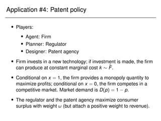
Application #4: Patent policy
 Players:
 Agent: Firm
 Planner: Regulator
 Designer: Patent agency
 Firm invests in a new technology; if investment is made, the firm
can produce at constant marginal cost k  F̃.
 Conditional on x = 1, the firm provides a monopoly quantity to
maximize profits; conditional on x = 0, the firm competes in a
competitive market. Market demand is D(p) = 1 p.
 The regulator and the patent agency maximize consumer
surplus with weight ! (but attach a positive weight to revenue).
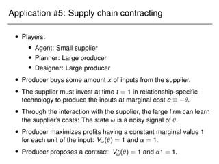
Application #5: Supply chain contracting
 Players:
 Agent: Small supplier
 Planner: Large producer
 Designer: Large producer
 Producer buys some amount x of inputs from the supplier.
 The supplier must invest at time t = 1 in relationship-specific
technology to produce the inputs at marginal cost c  .
 Through the interaction with the supplier, the large firm can learn
the supplier’s costs: The state ! is a noisy signal of .
 Producer maximizes profits having a constant marginal value 1
for each unit of the input: V!() = 1 and = 1:
 Producer proposes a contract: V?
!() = 1 and ?
= 1.
Analysis and results
Main result
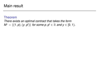
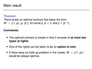
Theorem
There exists an optimal contract that takes the form
M?
= f(1;p);(y;p0)g for some p;p0 2 R and y 2 [0;1).
Main result
Theorem
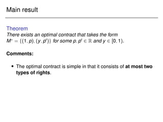
There exists an optimal contract that takes the form
M?
= f(1;p);(y;p0)g for some p;p0 2 R and y 2 [0;1).
Comments:
 The optimal contract is simple in that it consists of at most two
types of rights.
Main result
Theorem
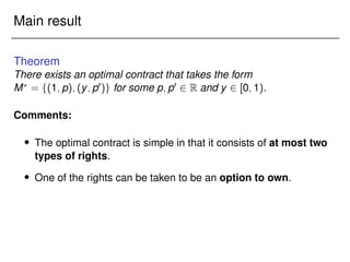
There exists an optimal contract that takes the form
M?
= f(1;p);(y;p0)g for some p;p0 2 R and y 2 [0;1).
Comments:
 The optimal contract is simple in that it consists of at most two
types of rights.
 One of the rights can be taken to be an option to own.
Main result
Theorem
There exists an optimal contract that takes the form
M?
= f(1;p);(y;p0)g for some p;p0 2 R and y 2 [0;1).
Comments:
 The optimal contract is simple in that it consists of at most two
types of rights.
 One of the rights can be taken to be an option to own.
 If there were no hold-up problem in the model, M?
= f(1; p)g
would be always optimal.
Step 1: Outside option constraint
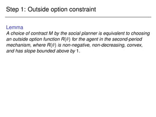
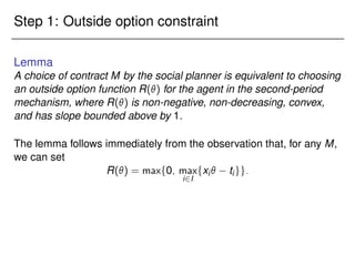
Lemma
A choice of contract M by the social planner is equivalent to choosing
an outside option function R() for the agent in the second-period
mechanism, where R() is non-negative, non-decreasing, convex,
and has slope bounded above by 1.
Step 1: Outside option constraint
Lemma
A choice of contract M by the social planner is equivalent to choosing
an outside option function R() for the agent in the second-period
mechanism, where R() is non-negative, non-decreasing, convex,
and has slope bounded above by 1.
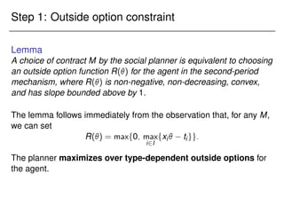
The lemma follows immediately from the observation that, for any M,
we can set
R() = maxf0; max
i2I
fxi tigg:
The planner maximizes over type-dependent outside options for
the agent.
Step 1: Outside option constraint
Fixing ! (and dropping it from the notation), the designer solves:
max
x:Θ![0;1]; u0
Z 

W()x()d u
s.t. x is non-decreasing;
U()  u +
Z 

x() d  R(); 8 2 Θ;
where
W()  (V() + B()) f();
and
B() = 
1 F()
f()
:
Step 1: Outside option constraint
Fixing ! (and dropping it from the notation), the designer solves:
max
x:Θ![0;1]; u0
Z 

W()x()d u
s.t. x is non-decreasing;
U()  u +
Z 

x() d  R(); 8 2 Θ;
where
W()  (V() + B()) f();
and
B() = 
1 F()
f()
:
This is a problem considered by Jullien (2000).
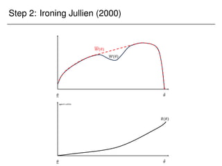
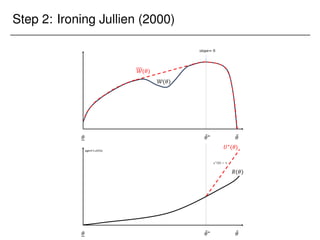
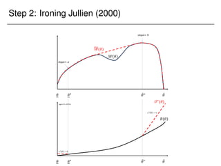
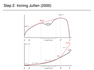
Step 2: Ironing Jullien (2000)
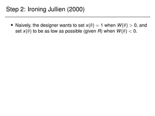
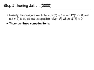
 Naively, the designer wants to set x() = 1 when W()  0, and
set x() to be as low as possible (given R) when W()  0.
Step 2: Ironing Jullien (2000)
 Naively, the designer wants to set x() = 1 when W()  0, and
set x() to be as low as possible (given R) when W()  0.
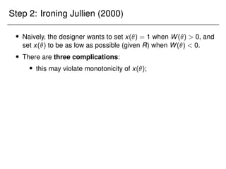
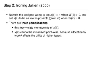
 There are three complications:
Step 2: Ironing Jullien (2000)
 Naively, the designer wants to set x() = 1 when W()  0, and
set x() to be as low as possible (given R) when W()  0.
 There are three complications:
 this may violate monotonicity of x();
Step 2: Ironing Jullien (2000)
 Naively, the designer wants to set x() = 1 when W()  0, and
set x() to be as low as possible (given R) when W()  0.
 There are three complications:
 this may violate monotonicity of x();
 x() cannot be minimized point-wise, because allocation to
type  affects the utility of higher types;
 the designer may want to use the transfer to satisfy the
outside-option constraint.
 These complications can be addressed by adapting the ironing
technique from Myerson (1981).
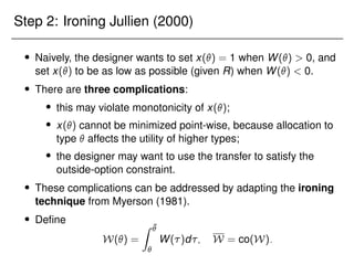
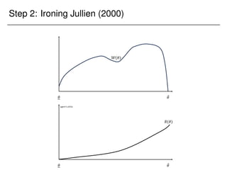
 Define
W() =
Z ¯


W()d; W = co(W):
Step 2: Ironing Jullien (2000)
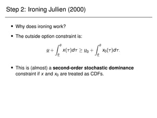
 Why does ironing work?
Step 2: Ironing Jullien (2000)
 Why does ironing work?
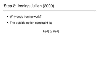
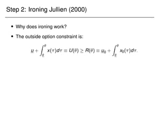
 The outside option constraint is:
u +
Z 

x()d U()  R() u0 +
Z 

x0()d:
Step 2: Ironing Jullien (2000)
 Why does ironing work?
 The outside option constraint is:
u +
Z 

x()d  U()  R()  u0 +
Z 

x0()d:
Step 2: Ironing Jullien (2000)
 Why does ironing work?
 The outside option constraint is:
u +
Z 

x()d  u0 +
Z 

x0()d:
Step 2: Ironing Jullien (2000)
 Why does ironing work?
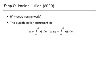
 The outside option constraint is:
u +
Z 

x()d  u0 +
Z 

x0()d:
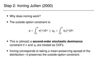
 This is (almost) a second-order stochastic dominance
constraint if x and x0 are treated as CDFs.
Step 2: Ironing Jullien (2000)
 Why does ironing work?
 The outside option constraint is:
u +
Z 

x()d  u0 +
Z 

x0()d:
 This is (almost) a second-order stochastic dominance
constraint if x and x0 are treated as CDFs.
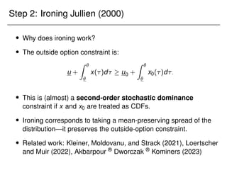
 Ironing corresponds to taking a mean-preserving spread of the
distribution—it preserves the outside-option constraint.
 Related work: Kleiner, Moldovanu, and Strack (2021), Loertscher
and Muir (2022), Akbarpour ® Dworczak ® Kominers (2023)
Step 3: Linearity of the planner’s problem
We now go back to t = 0.
Step 3: Linearity of the planner’s problem
We now go back to t = 0.
Lemma (Linearity)
The planner’s problem of choosing the optimal contract M is linear in
the outside option R().
Step 3: Linearity of the planner’s problem
We now go back to t = 0.
Lemma (Linearity)
The planner’s problem of choosing the optimal contract M is linear in
the outside option R().
 By the above construction, the optimal allocation rule x?
() for
the designer depends linearly on R().
Step 3: Linearity of the planner’s problem
We now go back to t = 0.
Lemma (Linearity)
The planner’s problem of choosing the optimal contract M is linear in
the outside option R().
 By the above construction, the optimal allocation rule x?
() for
the designer depends linearly on R().
 Key intuition: The set of types at which the outside-option
constraint binds is pinned down by the distribution of agent’s type
and designer’s preferences—it does not depend on R itself!
 Both the planner’s objective and the agent’s
investment-obedience constraint are linear in x?
.
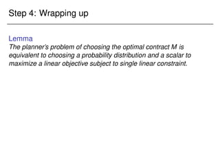
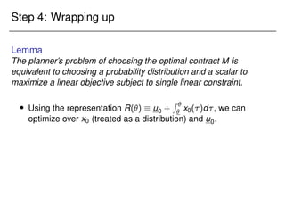
Step 4: Wrapping up
Lemma
The planner’s problem of choosing the optimal contract M is
equivalent to choosing a probability distribution and a scalar to
maximize a linear objective subject to single linear constraint.
Step 4: Wrapping up
Lemma
The planner’s problem of choosing the optimal contract M is
equivalent to choosing a probability distribution and a scalar to
maximize a linear objective subject to single linear constraint.
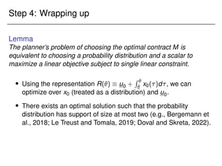
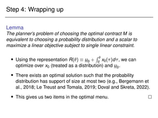
 Using the representation R()  u0 +
R 
 x0()d, we can
optimize over x0 (treated as a distribution) and u0.
 There exists an optimal solution such that the probability
distribution has support of size at most two (e.g., Bergemann et
al., 2018; Le Treust and Tomala, 2019; Doval and Skreta, 2022).
 This gives us two items in the optimal menu.
Corollaries of the proof
 With no constraint, the problem is to maximize a linear objective
=) solution is an extreme point
=) option to own is optimal.
Corollaries of the proof
 With no constraint, the problem is to maximize a linear objective
=) solution is an extreme point
=) option to own is optimal.
 Easy extension to K linear constraints
=) We need at most K + 1 options in the optimal menu.
Corollaries of the proof
 With no constraint, the problem is to maximize a linear objective
=) solution is an extreme point
=) option to own is optimal.
 Easy extension to K linear constraints
=) We need at most K + 1 options in the optimal menu.
 Extension to continuous investment:
Corollaries of the proof
 With no constraint, the problem is to maximize a linear objective
=) solution is an extreme point
=) option to own is optimal.
 Easy extension to K linear constraints
=) We need at most K + 1 options in the optimal menu.
 Extension to continuous investment:
 Suppose agent chooses e 2 [0; 1] at strictly convex cost
c(e), and e is the probability that  is drawn from F!.
Corollaries of the proof
 With no constraint, the problem is to maximize a linear objective
=) solution is an extreme point
=) option to own is optimal.
 Easy extension to K linear constraints
=) We need at most K + 1 options in the optimal menu.
 Extension to continuous investment:
 Suppose agent chooses e 2 [0; 1] at strictly convex cost
c(e), and e is the probability that  is drawn from F!.
 Satisfying FOC at the target investment level e?
is sufficient
for obedience.
Corollaries of the proof
 With no constraint, the problem is to maximize a linear objective
=) solution is an extreme point
=) option to own is optimal.
 Easy extension to K linear constraints
=) We need at most K + 1 options in the optimal menu.
 Extension to continuous investment:
 Suppose agent chooses e 2 [0; 1] at strictly convex cost
c(e), and e is the probability that  is drawn from F!.
 Satisfying FOC at the target investment level e?
is sufficient
for obedience.
 FOC is linear in R() =) we need two options in the
optimal menu.
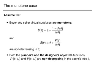
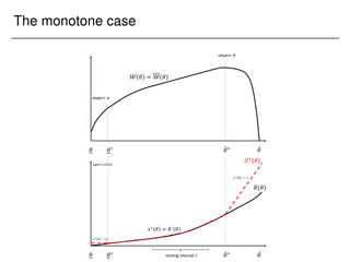
The monotone case
Assume that:
 Buyer and seller virtual surpluses are monotone:
B()  
1 F()
f()
and
S()   +
F()
f()
are non-decreasing in ;
 Both the planner’s and the designer’s objective functions
V?
(; !) and V(; !) are non-decreasing in the agent’s type .
The monotone case
The monotone case
Lemma (The monotone case)
For any outside option function R(), the mechanism designer in the
second period will choose an optimal mechanism in which the
outside-option constraint binds for types in the interval [?
!; ¯
?
!].
The monotone case
Lemma (The monotone case)
For any outside option function R(), the mechanism designer in the
second period will choose an optimal mechanism in which the
outside-option constraint binds for types in the interval [?
!; ¯
?
!].
Moreover, except for the case of a boundary solution,
V(?
!; !) + S(?
!) = 0;
V(¯
?
!; !) + B(¯
?
!) = 0:
 For   ¯
?
!, the designer wants to allocate the good to the agent
anyway, so the outside-option constraint is slack;
 For   ?
!, the designer prefers to “buy out” the rights using a
monetary payment, so the constraint is again slack.
The monotone case
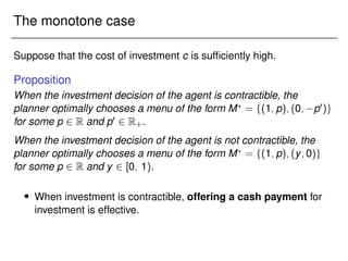
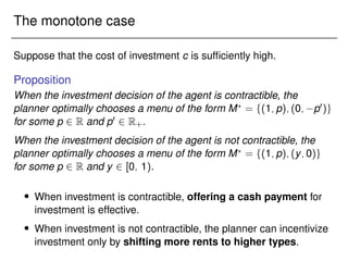
Suppose that the cost of investment c is sufficiently high.
The monotone case
Suppose that the cost of investment c is sufficiently high.
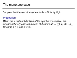
Proposition
When the investment decision of the agent is contractible, the
planner optimally chooses a menu of the form M?
= f(1;p);(0; p0)g
for some p 2 R and p0 2 R+.
The monotone case
Suppose that the cost of investment c is sufficiently high.
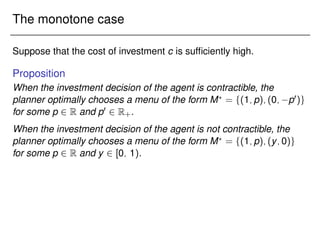
Proposition
When the investment decision of the agent is contractible, the
planner optimally chooses a menu of the form M?
= f(1;p);(0; p0)g
for some p 2 R and p0 2 R+.
When the investment decision of the agent is not contractible, the
planner optimally chooses a menu of the form M?
= f(1;p);(y;0)g
for some p 2 R and y 2 [0; 1).
 When investment is contractible, offering a cash payment for
investment is effective.
 When investment is not contractible, the planner can incentivize
investment only by shifting more rents to higher types.
Applications
Applications
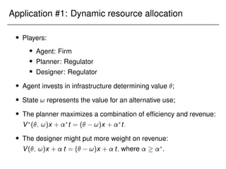
Application #1: Dynamic resource allocation
 Players:
 Agent: Firm
 Planner: Regulator
 Designer: Regulator
 Agent invests in infrastructure determining value ;
 State ! represents the value for an alternative use;
 The planner maximizes a combination of efficiency and revenue:
V?
(; !)x + ?
t = ( !)x + ?
t:
 The designer might put more weight on revenue:
V(; !)x + t = ( !)x + t; where  ?
.
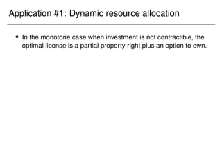
Application #1: Dynamic resource allocation
 In the monotone case when investment is not contractible, the
optimal license is a partial property right plus an option to own.
Application #1: Dynamic resource allocation
 In the monotone case when investment is not contractible, the
optimal license is a partial property right plus an option to own.
 Suppose that F! is uniform on [0; 1], and F! is an atom at 0.
Application #1: Dynamic resource allocation
 In the monotone case when investment is not contractible, the
optimal license is a partial property right plus an option to own.
 Suppose that F! is uniform on [0; 1], and F! is an atom at 0.
 The optimal property right as a function of value for revenue:
 = ?
= 1: option to own (1; p)
(p makes the investment-obedience constraint bind);
 = 1; ?
= 0: partial property right (0; y)
(y makes the investment-obedience constraint bind);
 = ?
= 0: no right
(consistent with Rogerson (1992))
Application #2: Regulating a private rental market
 Players:
 Agent: Tenant
 Planner: Regulator
 Designer: Rental company
 Agent invests in the property determining her value  for staying.
 The state ! is the seller’s outside option (market rental price).
 The seller wants to maximize revenue:
V(; !)x + t = !x + t.
 The planner wants to maximize efficiency:
V?
(; !)x + ?
t = ( !)x:
Application #2: Regulating a private rental market
 Suppose that without investment, value  is uniform on [0; 1];
with investment, the value is drawn from [∆; 1 + ∆] instead.
Application #2: Regulating a private rental market
 Suppose that without investment, value  is uniform on [0; 1];
with investment, the value is drawn from [∆; 1 + ∆] instead.
 Suppose that ! is known (and lies in a certain range).
Application #2: Regulating a private rental market
 Suppose that without investment, value  is uniform on [0; 1];
with investment, the value is drawn from [∆; 1 + ∆] instead.
 Suppose that ! is known (and lies in a certain range).
 The optimal contract is a renewable lease with price
p?
= ! ∆;
where is the Lagrange multiplier on the investment constraint.
 If investment constraint is slack, p?
= !, so the planner “forces”
the seller to use a VCG mechanism.
 If ! is random, then (assuming interior solution)
p?
= E[ ! j ?
!  p?
 ?
!] ∆:
Application #3: Vaccine development
 Players:
 Agent: Pharmaceutical company
 Planner: Health agency
 Designer: Health agency
 Company develops a vaccine; the marginal cost of production
conditional on investment is k  e
F ( = k);
 Allocation x is the number of units purchased by the health
agency, with 1 being the mass of the patient population;
 Health agency maximizes the total value of allocation,
V?
(; !)x = V(; !)x = !x,
where ! measures the severity of the health crisis.
 Assume that 1 =  ?
.
Application #3: Vaccine development
 Assume that investment is observable and that ! is known.
Application #3: Vaccine development
 Assume that investment is observable and that ! is known.
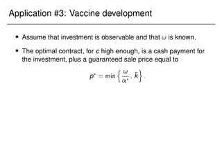
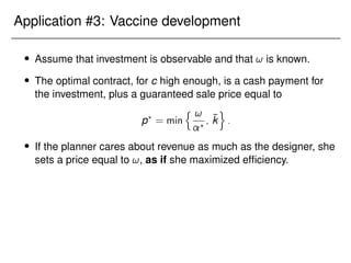
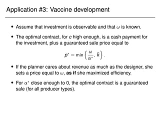
 The optimal contract, for c high enough, is a cash payment for
the investment, plus a guaranteed sale price equal to
p?
= min
n !
?
; k̄
o
:
Application #3: Vaccine development
 Assume that investment is observable and that ! is known.
 The optimal contract, for c high enough, is a cash payment for
the investment, plus a guaranteed sale price equal to
p?
= min
n !
?
; k̄
o
:
 If the planner cares about revenue as much as the designer, she
sets a price equal to !, as if she maximized efficiency.
 For ?
close enough to 0, the optimal contract is a guaranteed
sale (for all producer types).
Application #3: Vaccine development
 If ! is stochastic, then the optimal price satisfies
p?
= min
(
E

!j! 2 [!p? ; ¯
!p? ]

?
; k̄
)
;
where [!p? ; ¯
!p? ] is the interval of !’s for which the choice of p?
changes the second-period mechanism.
Application #3: Vaccine development
 If ! is stochastic, then the optimal price satisfies
p?
= min
(
E

!j! 2 [!p? ; ¯
!p? ]

?
; k̄
)
;
where [!p? ; ¯
!p? ] is the interval of !’s for which the choice of p?
changes the second-period mechanism.
 If the realized ! is high (health crisis is severe), the designer will
offer a price better than p?
.
Application #3: Vaccine development
 If ! is stochastic, then the optimal price satisfies
p?
= min
(
E

!j! 2 [!p? ; ¯
!p? ]

?
; k̄
)
;
where [!p? ; ¯
!p? ] is the interval of !’s for which the choice of p?
changes the second-period mechanism.
 If the realized ! is high (health crisis is severe), the designer will
offer a price better than p?
.
 If the realized ! is low (health crisis is mild), the designer will
offer a price lower than p?
and compensate the producer with an
additional cash payment (on top of the payment for investment).
Application #4: Patent policy
 Players:
 Agent: Firm
 Planner: Regulator
 Designer: Patent agency
 Firm invests in a new technology; if investment is made, the firm
can produce at constant marginal cost k  F̃.
 Conditional on x = 1, the firm provides a monopoly quantity to
maximize profits; conditional on x = 0, the firm competes in a
competitive market. Market demand is D(p) = 1 p.
 The regulator and the patent agency maximize consumer
surplus with weight ! (but attach a positive weight to revenue).
Application #4: Patent policy
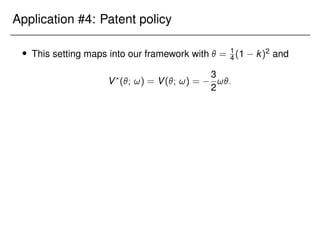
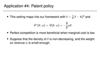
 This setting maps into our framework with  = 1
4 (1 k)2 and
V?
(; !) = V(; !) =
3
2
!:
Application #4: Patent policy
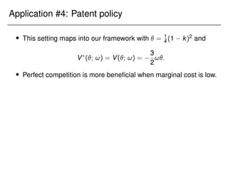
 This setting maps into our framework with  = 1
4 (1 k)2 and
V?
(; !) = V(; !) =
3
2
!:
 Perfect competition is more beneficial when marginal cost is low.
Application #4: Patent policy
 This setting maps into our framework with  = 1
4 (1 k)2 and
V?
(; !) = V(; !) =
3
2
!:
 Perfect competition is more beneficial when marginal cost is low.
 Suppose that the density of  is non-decreasing, and the weight
on revenue is small enough.
Application #4: Patent policy
 This setting maps into our framework with  = 1
4 (1 k)2 and
V?
(; !) = V(; !) =
3
2
!:
 Perfect competition is more beneficial when marginal cost is low.
 Suppose that the density of  is non-decreasing, and the weight
on revenue is small enough.
 Then, an optimal contract is to offer full patent protection to the
invention (x = 1) with exogenous probability y 2 (0; 1] at no
payment.
Application #5: Supply chain contracting
 Players:
 Agent: Small supplier
 Planner: Large producer
 Designer: Large producer
 Producer buys some amount x of inputs from the supplier.
 The supplier must invest at time t = 1 in relationship-specific
technology to produce the inputs at marginal cost c  .
 Through the interaction with the supplier, the large firm can learn
the supplier’s costs: The state ! is a noisy signal of .
 Producer maximizes profits having a constant marginal value 1
for each unit of the input: V!() = 1 and = 1:
 Producer proposes a contract: V?
!() = 1 and ?
= 1.
Application #5: Supply chain contracting
 Suppose investment by the small supplier is not contractible.
Application #5: Supply chain contracting
 Suppose investment by the small supplier is not contractible.
 The producer will in general commit to a two-price scheme,
committing to buy up to y units at some price pH, and any
number of units at some lower price pL.
Application #5: Supply chain contracting
 Suppose investment by the small supplier is not contractible.
 The producer will in general commit to a two-price scheme,
committing to buy up to y units at some price pH, and any
number of units at some lower price pL.
 If investment by the small supplier is contractible, assuming the
cost of investment is high enough, the producer will offer an
upfront payment for setting up production and a guaranteed
purchase price for any number of units.
Summary and future steps
Summary
 We introduced a simple but flexible framework for analyzing
optimal design of (property) rights.
Summary
 We introduced a simple but flexible framework for analyzing
optimal design of (property) rights.
 Optimally designed rights partially restore commitment to
future trading mechanisms.
Summary
 We introduced a simple but flexible framework for analyzing
optimal design of (property) rights.
 Optimally designed rights partially restore commitment to
future trading mechanisms.
 The optimal right often features an option to own.
Future steps
 Maskin-Tirole (1999) critique of incomplete contracts: Can the
planner do better by conditioning rights on the state in an
incentive-compatible way?
Future steps
 Maskin-Tirole (1999) critique of incomplete contracts: Can the
planner do better by conditioning rights on the state in an
incentive-compatible way?
 Consider designing a menu of menus M = fMjgj such that the
designer selects a menu Mj based on realized state and the
agent chooses an option from Mj.
Future steps
 Maskin-Tirole (1999) critique of incomplete contracts: Can the
planner do better by conditioning rights on the state in an
incentive-compatible way?
 Consider designing a menu of menus M = fMjgj such that the
designer selects a menu Mj based on realized state and the
agent chooses an option from Mj. This can help!
 What if both parties (at t = 2) have private information and
bargaining power is not exogenous?
Future steps
 Maskin-Tirole (1999) critique of incomplete contracts: Can the
planner do better by conditioning rights on the state in an
incentive-compatible way?
 Consider designing a menu of menus M = fMjgj such that the
designer selects a menu Mj based on realized state and the
agent chooses an option from Mj. This can help!
 What if both parties (at t = 2) have private information and
bargaining power is not exogenous? Allocate rights to both
parties?
 Optimal allocation of contracts at t = 0 to multiple agents?

Presentation_Columbia.pdf

  • 1.
    A mechanism-design approachto property rights Piotr Dworczak? Ellen Muir (Northwestern; GRAPE) (Harvard) October 9, 2023 Economic Theory Workshop, Columbia University ? Co-funded by the European Union (ERC, IMD-101040122). Views and opinions expressed are those of the authors only and do not necessarily reflect those of the European Union or the European Research Council.
  • 2.
    Motivation Vast literaturein mechanism design studies the problem of optimal allocation of economic resources.
  • 3.
    Motivation Vast literaturein mechanism design studies the problem of optimal allocation of economic resources. Less is known about how to design the contractual rights relating to the control of the resource (“property rights”).
  • 4.
    Motivation Vast literaturein mechanism design studies the problem of optimal allocation of economic resources. Less is known about how to design the contractual rights relating to the control of the resource (“property rights”). Example:
  • 5.
    Motivation Vast literaturein mechanism design studies the problem of optimal allocation of economic resources. Less is known about how to design the contractual rights relating to the control of the resource (“property rights”). Example: Selling an apple...
  • 6.
    Motivation Vast literaturein mechanism design studies the problem of optimal allocation of economic resources. Less is known about how to design the contractual rights relating to the control of the resource (“property rights”). Example: Selling an apple... ... versus selling a spectrum license.
  • 7.
    Motivation Vast literaturein mechanism design studies the problem of optimal allocation of economic resources. Less is known about how to design the contractual rights relating to the control of the resource (“property rights”). Example: Selling an apple... ... versus selling a spectrum license. We provide a framework for studying optimal design of contractual rights.
  • 8.
    Key features ofour framework In our framework, property rights determine the holder’s outside options (with regard to the underlying good) in economic interactions:
  • 9.
    Key features ofour framework In our framework, property rights determine the holder’s outside options (with regard to the underlying good) in economic interactions: Full property right: Holder can always keep the good;
  • 10.
    Key features ofour framework In our framework, property rights determine the holder’s outside options (with regard to the underlying good) in economic interactions: Full property right: Holder can always keep the good; No rights: Outside option is (normalized to) zero;
  • 11.
    Key features ofour framework In our framework, property rights determine the holder’s outside options (with regard to the underlying good) in economic interactions: Full property right: Holder can always keep the good; No rights: Outside option is (normalized to) zero; Renewable lease: Holder can keep the good at a price;
  • 12.
    Key features ofour framework In our framework, property rights determine the holder’s outside options (with regard to the underlying good) in economic interactions: Full property right: Holder can always keep the good; No rights: Outside option is (normalized to) zero; Renewable lease: Holder can keep the good at a price; ...
  • 13.
    Key features ofour framework In our framework, property rights determine the holder’s outside options (with regard to the underlying good) in economic interactions: Full property right: Holder can always keep the good; No rights: Outside option is (normalized to) zero; Renewable lease: Holder can keep the good at a price; ... We model the economic interaction as the holder of the rights participating in a trading mechanism.
  • 14.
    Key features ofour framework Fundamental friction: Social planner cannot commit to future trading mechanisms, resulting in
  • 15.
    Key features ofour framework Fundamental friction: Social planner cannot commit to future trading mechanisms, resulting in ex-post inefficiency (mechanism may be suboptimal);
  • 16.
    Key features ofour framework Fundamental friction: Social planner cannot commit to future trading mechanisms, resulting in ex-post inefficiency (mechanism may be suboptimal); hold-up problem (inefficient investment decisions).
  • 17.
    Key features ofour framework Fundamental friction: Social planner cannot commit to future trading mechanisms, resulting in ex-post inefficiency (mechanism may be suboptimal); hold-up problem (inefficient investment decisions). Planner chooses property rights to alleviate these frictions.
  • 18.
    Key features ofour framework Fundamental friction: Social planner cannot commit to future trading mechanisms, resulting in ex-post inefficiency (mechanism may be suboptimal); hold-up problem (inefficient investment decisions). Planner chooses property rights to alleviate these frictions. Question: What is the optimal set of rights?
  • 19.
    Key features ofour framework Fundamental friction: Social planner cannot commit to future trading mechanisms, resulting in ex-post inefficiency (mechanism may be suboptimal); hold-up problem (inefficient investment decisions). Planner chooses property rights to alleviate these frictions. Question: What is the optimal set of rights? Main result: The optimal property right is simple but flexible, often featuring an option to own.
  • 20.
    Property rights ineconomics Coase (1960): Any assignment of property rights leads to efficient outcomes as long as there are transaction costs.
  • 21.
    Property rights ineconomics Coase (1960): Any assignment of property rights leads to efficient outcomes as long as there are transaction costs. Williamson (1979): Transaction costs take center stage in economics.
  • 22.
    Property rights ineconomics Coase (1960): Any assignment of property rights leads to efficient outcomes as long as there are transaction costs. Williamson (1979): Transaction costs take center stage in economics. Two large literatures:
  • 23.
    Property rights ineconomics Coase (1960): Any assignment of property rights leads to efficient outcomes as long as there are transaction costs. Williamson (1979): Transaction costs take center stage in economics. Two large literatures: Property rights affect efficiency under private information:
  • 24.
    Property rights ineconomics Coase (1960): Any assignment of property rights leads to efficient outcomes as long as there are transaction costs. Williamson (1979): Transaction costs take center stage in economics. Two large literatures: Property rights affect efficiency under private information: Myerson and Satterthwaite (1983);
  • 25.
    Property rights ineconomics Coase (1960): Any assignment of property rights leads to efficient outcomes as long as there are transaction costs. Williamson (1979): Transaction costs take center stage in economics. Two large literatures: Property rights affect efficiency under private information: Myerson and Satterthwaite (1983); Cramton, Gibbons and Klemperer (1987), ...
  • 26.
    Property rights ineconomics Coase (1960): Any assignment of property rights leads to efficient outcomes as long as there are transaction costs. Williamson (1979): Transaction costs take center stage in economics. Two large literatures: Property rights affect efficiency under private information: Myerson and Satterthwaite (1983); Cramton, Gibbons and Klemperer (1987), ... Property rights affect investment incentives:
  • 27.
    Property rights ineconomics Coase (1960): Any assignment of property rights leads to efficient outcomes as long as there are transaction costs. Williamson (1979): Transaction costs take center stage in economics. Two large literatures: Property rights affect efficiency under private information: Myerson and Satterthwaite (1983); Cramton, Gibbons and Klemperer (1987), ... Property rights affect investment incentives: Grossman and Hart (1986), Hart and Moore (1990), Aghion, Dewatripont and Rey (1994), Maskin and Tirole (1999), ...
  • 28.
    Marginal contribution Westudy both effects in a setting with one-sided private information and exogenous distribution of bargaining power.
  • 29.
    Marginal contribution Westudy both effects in a setting with one-sided private information and exogenous distribution of bargaining power. To the best of our knowledge, our paper is first to characterize the optimal property right from a non-parametric class (in a setting where the first best cannot in general be achieved).
  • 30.
    Marginal contribution Westudy both effects in a setting with one-sided private information and exogenous distribution of bargaining power. To the best of our knowledge, our paper is first to characterize the optimal property right from a non-parametric class (in a setting where the first best cannot in general be achieved). Attractive properties of option-to-own contracts were studied:
  • 31.
    Marginal contribution Westudy both effects in a setting with one-sided private information and exogenous distribution of bargaining power. To the best of our knowledge, our paper is first to characterize the optimal property right from a non-parametric class (in a setting where the first best cannot in general be achieved). Attractive properties of option-to-own contracts were studied: Liability rules raise second-best efficiency in bargaining.
  • 32.
    Marginal contribution Westudy both effects in a setting with one-sided private information and exogenous distribution of bargaining power. To the best of our knowledge, our paper is first to characterize the optimal property right from a non-parametric class (in a setting where the first best cannot in general be achieved). Attractive properties of option-to-own contracts were studied: Liability rules raise second-best efficiency in bargaining. - Che (2006), Segal and Whinston (2016)
  • 33.
    Marginal contribution Westudy both effects in a setting with one-sided private information and exogenous distribution of bargaining power. To the best of our knowledge, our paper is first to characterize the optimal property right from a non-parametric class (in a setting where the first best cannot in general be achieved). Attractive properties of option-to-own contracts were studied: Liability rules raise second-best efficiency in bargaining. - Che (2006), Segal and Whinston (2016) Options to own may induce efficient investments.
  • 34.
    Marginal contribution Westudy both effects in a setting with one-sided private information and exogenous distribution of bargaining power. To the best of our knowledge, our paper is first to characterize the optimal property right from a non-parametric class (in a setting where the first best cannot in general be achieved). Attractive properties of option-to-own contracts were studied: Liability rules raise second-best efficiency in bargaining. - Che (2006), Segal and Whinston (2016) Options to own may induce efficient investments. - Hart (1995), Nöldeke and Schmidt (1995, 1998)
  • 35.
    Marginal contribution Westudy both effects in a setting with one-sided private information and exogenous distribution of bargaining power. To the best of our knowledge, our paper is first to characterize the optimal property right from a non-parametric class (in a setting where the first best cannot in general be achieved). Attractive properties of option-to-own contracts were studied: Liability rules raise second-best efficiency in bargaining. - Che (2006), Segal and Whinston (2016) Options to own may induce efficient investments. - Hart (1995), Nöldeke and Schmidt (1995, 1998) We provide an optimality foundation.
  • 36.
    Marginal contribution Thesetting allows us to study market-design applications:
  • 37.
    Marginal contribution Thesetting allows us to study market-design applications: optimal license design;
  • 38.
    Marginal contribution Thesetting allows us to study market-design applications: optimal license design; regulating a private rental market;
  • 39.
    Marginal contribution Thesetting allows us to study market-design applications: optimal license design; regulating a private rental market; optimal patent policy.
  • 40.
    Marginal contribution Thesetting allows us to study market-design applications: optimal license design; regulating a private rental market; optimal patent policy. On the technical side:
  • 41.
    Marginal contribution Thesetting allows us to study market-design applications: optimal license design; regulating a private rental market; optimal patent policy. On the technical side: We provide a novel solution method for mechanism design with type-dependent outside options (Lewis and Sappington, 1988, Jullien, 2000) based on an extension of the ironing technique (Myerson, 1981).
  • 42.
    Marginal contribution Thesetting allows us to study market-design applications: optimal license design; regulating a private rental market; optimal patent policy. On the technical side: We provide a novel solution method for mechanism design with type-dependent outside options (Lewis and Sappington, 1988, Jullien, 2000) based on an extension of the ironing technique (Myerson, 1981). We show how to optimize over the outside-option function.
  • 43.
    Other related papers Allocation mechanisms versus efficient investment: Rogerson (1992), Bergemann and Välimäki (2002), Milgrom (2017), Hatfield, Kojima, and Kominers (2019), Akbarpour, Kominers, Li, Li, and Milgrom (2023), ... Related techniques: Kleiner, Moldovanu, and Strack (2021), Loertscher and Muir (2022), Kang (2023), Akbarpour ® Dworczak ® Kominers (2023),... Spectrum license design: Milgrom, Weyl and Zhang (2017), Weyl and Zhang (2017), ... Optimal patent design: Matutes, Regibeau and Rockett (1996), Wright (1999), Hopenhayn, Llobet and Mitchell (2006), ...
  • 44.
  • 45.
    Model There isan agent, a designer, and a social planner;
  • 46.
    Model There isan agent, a designer, and a social planner; At time t = 0:
  • 47.
    Model There isan agent, a designer, and a social planner; At time t = 0: The planner designs a contract (set of rights) that the agent holds.
  • 48.
    Model There isan agent, a designer, and a social planner; At time t = 0: The planner designs a contract (set of rights) that the agent holds. At time t = 1:
  • 49.
    Model There isan agent, a designer, and a social planner; At time t = 0: The planner designs a contract (set of rights) that the agent holds. At time t = 1: The agent decides whether to invest at (sunk) cost c 0;
  • 50.
    Model There isan agent, a designer, and a social planner; At time t = 0: The planner designs a contract (set of rights) that the agent holds. At time t = 1: The agent decides whether to invest at (sunk) cost c 0; At time t = 2:
  • 51.
    Model There isan agent, a designer, and a social planner; At time t = 0: The planner designs a contract (set of rights) that the agent holds. At time t = 1: The agent decides whether to invest at (sunk) cost c 0; At time t = 2: The agent’s (privately observed) type and a public state ! are drawn from a joint distribution that depends on whether the agent invested or not.
  • 52.
    Model There isan agent, a designer, and a social planner; At time t = 0: The planner designs a contract (set of rights) that the agent holds. At time t = 1: The agent decides whether to invest at (sunk) cost c 0; At time t = 2: The agent’s (privately observed) type and a public state ! are drawn from a joint distribution that depends on whether the agent invested or not. The designer chooses a mechanism, and trade happens.
  • 53.
    Model Time t =2 continued: Designer chooses a trading mechanism (x!(); t!()), where x 2 [0; 1] denotes an allocation, and t 2 R denotes a transfer;
  • 54.
    Model Time t =2 continued: Designer chooses a trading mechanism (x!(); t!()), where x 2 [0; 1] denotes an allocation, and t 2 R denotes a transfer; Mechanism is chosen subject to IC and IR constraints, and must respect the rights that the agent holds.
  • 55.
    Model Time t =2 continued: Designer chooses a trading mechanism (x!(); t!()), where x 2 [0; 1] denotes an allocation, and t 2 R denotes a transfer; Mechanism is chosen subject to IC and IR constraints, and must respect the rights that the agent holds. Designer maximizes V(; !) x + t, where 0.
  • 56.
    Model Time t =2 continued: Designer chooses a trading mechanism (x!(); t!()), where x 2 [0; 1] denotes an allocation, and t 2 R denotes a transfer; Mechanism is chosen subject to IC and IR constraints, and must respect the rights that the agent holds. Designer maximizes V(; !) x + t, where 0. Agent’s utility is x t.
  • 57.
    Model Agent’s problem att = 1 The agent decides whether to pay the cost c 0 to invest.
  • 58.
    Model Agent’s problem att = 1 The agent decides whether to pay the cost c 0 to invest. If the agent invests:
  • 59.
    Model Agent’s problem att = 1 The agent decides whether to pay the cost c 0 to invest. If the agent invests: ! G, F!.
  • 60.
    Model Agent’s problem att = 1 The agent decides whether to pay the cost c 0 to invest. If the agent invests: ! G, F!. Otherwise:
  • 61.
    Model Agent’s problem att = 1 The agent decides whether to pay the cost c 0 to invest. If the agent invests: ! G, F!. Otherwise: ! G, F!, with F! FOSD F!, for every !.
  • 62.
    Model Agent’s problem att = 1 The agent decides whether to pay the cost c 0 to invest. If the agent invests: ! G, F!. Otherwise: ! G, F!, with F! FOSD F!, for every !. In the non-contractible case, the mechanism at t = 2 and the planner’s contract do not depend on the investment decision.
  • 63.
    Model Agent’s problem att = 1 The agent decides whether to pay the cost c 0 to invest. If the agent invests: ! G, F!. Otherwise: ! G, F!, with F! FOSD F!, for every !. In the non-contractible case, the mechanism at t = 2 and the planner’s contract do not depend on the investment decision. In the contractible case, the mechanism at t = 2 and the planner’s contract are contingent on the investment decision.
  • 64.
    Model Social planner’s problemat t = 0 Social planner chooses a contract that is a menu of “rights” M = f(xi; ti)gi2I; where xi 2 [0; 1], ti 2 R, and set I is arbitrary (M is compact).
  • 65.
    Model Social planner’s problemat t = 0 Social planner chooses a contract that is a menu of “rights” M = f(xi; ti)gi2I; where xi 2 [0; 1], ti 2 R, and set I is arbitrary (M is compact). The agent can “execute” any one of these rights at t = 2.
  • 66.
    Model Social planner’s problemat t = 0 Social planner chooses a contract that is a menu of “rights” M = f(xi; ti)gi2I; where xi 2 [0; 1], ti 2 R, and set I is arbitrary (M is compact). The agent can “execute” any one of these rights at t = 2. Social planner maximizes V? (; !)x + ? t, where ? 0.
  • 67.
    Model Social planner’s problemat t = 0 Social planner chooses a contract that is a menu of “rights” M = f(xi; ti)gi2I; where xi 2 [0; 1], ti 2 R, and set I is arbitrary (M is compact). The agent can “execute” any one of these rights at t = 2. Social planner maximizes V? (; !)x + ? t, where ? 0.
  • 68.
    Model Social planner’s problemat t = 0 Social planner chooses a contract that is a menu of “rights” M = f(xi; ti)gi2I; where xi 2 [0; 1], ti 2 R, and set I is arbitrary (M is compact). The agent can “execute” any one of these rights at t = 2. Social planner maximizes V? (; !)x + ? t, where ? 0. Assume: Investment is preferred by the social planner to no investment; investment can be induced by some contract; but it is not induced if the agent holds no rights.
  • 69.
    Model Social planner’s problemat t = 0 Social planner chooses a contract that is a menu of “rights” M = f(xi; ti)gi2I; where xi 2 [0; 1], ti 2 R, and set I is arbitrary (M is compact). The agent can “execute” any one of these rights at t = 2. Social planner maximizes V? (; !)x + ? t, where ? 0. Technicalities: Θ [; ¯ ] is a compact subset of R; V and V? are continuous in (and measurable in !), F has a continuous positive density on Θ.
  • 70.
    Comments about themodel A contract creates an outside option for the agent: Designer must guarantee that the agent’s type- utility from participating in the mechanism is not lower than max i2I fxi tig:
  • 71.
    Comments about themodel A contract creates an outside option for the agent: Designer must guarantee that the agent’s type- utility from participating in the mechanism is not lower than max i2I fxi tig: The framework captures many conventional rights:
  • 72.
    Comments about themodel A contract creates an outside option for the agent: Designer must guarantee that the agent’s type- utility from participating in the mechanism is not lower than max i2I fxi tig: The framework captures many conventional rights: Property right: M = f(x = 1; t = 0)g;
  • 73.
    Comments about themodel A contract creates an outside option for the agent: Designer must guarantee that the agent’s type- utility from participating in the mechanism is not lower than max i2I fxi tig: The framework captures many conventional rights: Property right: M = f(x = 1; t = 0)g; Cash payment: M = f(0; p)g;
  • 74.
    Comments about themodel A contract creates an outside option for the agent: Designer must guarantee that the agent’s type- utility from participating in the mechanism is not lower than max i2I fxi tig: The framework captures many conventional rights: Property right: M = f(x = 1; t = 0)g; Cash payment: M = f(0; p)g; Property right with a resale option: M = f(1;0); (0; p)g;
  • 75.
    Comments about themodel A contract creates an outside option for the agent: Designer must guarantee that the agent’s type- utility from participating in the mechanism is not lower than max i2I fxi tig: The framework captures many conventional rights: Property right: M = f(x = 1; t = 0)g; Cash payment: M = f(0; p)g; Property right with a resale option: M = f(1;0); (0; p)g; Renewable lease/ option to own: M = f(1; p)g;
  • 76.
    Comments about themodel A contract creates an outside option for the agent: Designer must guarantee that the agent’s type- utility from participating in the mechanism is not lower than max i2I fxi tig: The framework captures many conventional rights: Property right: M = f(x = 1; t = 0)g; Cash payment: M = f(0; p)g; Property right with a resale option: M = f(1;0); (0; p)g; Renewable lease/ option to own: M = f(1; p)g; Partial property right: M = f(y; 0)g, where y 2 (0; 1);
  • 77.
    Comments about themodel A contract creates an outside option for the agent: Designer must guarantee that the agent’s type- utility from participating in the mechanism is not lower than max i2I fxi tig: The framework captures many conventional rights: Property right: M = f(x = 1; t = 0)g; Cash payment: M = f(0; p)g; Property right with a resale option: M = f(1;0); (0; p)g; Renewable lease/ option to own: M = f(1; p)g; Partial property right: M = f(y; 0)g, where y 2 (0; 1); Flexible property right: M = fs; p(s))gs2[0; 1].
  • 78.
    Comments about themodel There are two frictions in the model:
  • 79.
    Comments about themodel There are two frictions in the model: 1. Divergence of preferences between the planner and designer (“ex-post inefficiency”);
  • 80.
    Comments about themodel There are two frictions in the model: 1. Divergence of preferences between the planner and designer (“ex-post inefficiency”); 2. Non-contractible investment decision (“hold-up problem”);
  • 81.
    Comments about themodel There are two frictions in the model: 1. Divergence of preferences between the planner and designer (“ex-post inefficiency”); 2. Non-contractible investment decision (“hold-up problem”); Additionally, we limited the power of property rights by assuming that they cannot be state-contingent (“incomplete contracts”);
  • 82.
    Comments about themodel There are two frictions in the model: 1. Divergence of preferences between the planner and designer (“ex-post inefficiency”); 2. Non-contractible investment decision (“hold-up problem”); Additionally, we limited the power of property rights by assuming that they cannot be state-contingent (“incomplete contracts”); We can “switch off” some frictions and provide tighter results.
  • 83.
    Comments about themodel There are two frictions in the model: 1. Divergence of preferences between the planner and designer (“ex-post inefficiency”); 2. Non-contractible investment decision (“hold-up problem”); Additionally, we limited the power of property rights by assuming that they cannot be state-contingent (“incomplete contracts”); We can “switch off” some frictions and provide tighter results. Uninteresting cases:
  • 84.
    Comments about themodel There are two frictions in the model: 1. Divergence of preferences between the planner and designer (“ex-post inefficiency”); 2. Non-contractible investment decision (“hold-up problem”); Additionally, we limited the power of property rights by assuming that they cannot be state-contingent (“incomplete contracts”); We can “switch off” some frictions and provide tighter results. Uninteresting cases: If there is no investment and the planner and designer are aligned, it is optimal to allocate no rights to the agent.
  • 85.
    Comments about themodel There are two frictions in the model: 1. Divergence of preferences between the planner and designer (“ex-post inefficiency”); 2. Non-contractible investment decision (“hold-up problem”); Additionally, we limited the power of property rights by assuming that they cannot be state-contingent (“incomplete contracts”); We can “switch off” some frictions and provide tighter results. Uninteresting cases: If there is no investment and the planner and designer are aligned, it is optimal to allocate no rights to the agent. If the designer did not care about her revenue ( = 0), she would “buy out” the agent’s rights.
  • 86.
    Application #1: Dynamicresource allocation Players: Agent: Firm Planner: Regulator Designer: Regulator Agent invests in infrastructure determining value ; State ! represents the value for an alternative use; The planner maximizes a combination of efficiency and revenue: V? (; !)x + ? t = ( !)x + ? t: The designer might put more weight on revenue: V(; !)x + t = ( !)x + t; where ? .
  • 87.
    Application #2: Regulatinga private rental market Players: Agent: Tenant Planner: Regulator Designer: Rental company Agent invests in the property determining her value for staying. The state ! is the seller’s outside option (market rental price). The seller wants to maximize revenue: V(; !)x + t = !x + t. The planner wants to maximize efficiency: V? (; !)x + ? t = ( !)x:
  • 88.
    Application #3: Vaccinedevelopment Players: Agent: Pharmaceutical company Planner: Health agency Designer: Health agency Company develops a vaccine; the marginal cost of production conditional on investment is k F̃ ( = k); Allocation x is the number of units purchased by the health agency, with 1 being the mass of the patient population; Health agency maximizes the total value of allocation, V? (; !)x = V(; !)x = !x, where ! measures the severity of the health crisis.
  • 89.
    Application #4: Patentpolicy Players: Agent: Firm Planner: Regulator Designer: Patent agency Firm invests in a new technology; if investment is made, the firm can produce at constant marginal cost k F̃. Conditional on x = 1, the firm provides a monopoly quantity to maximize profits; conditional on x = 0, the firm competes in a competitive market. Market demand is D(p) = 1 p. The regulator and the patent agency maximize consumer surplus with weight ! (but attach a positive weight to revenue).
  • 90.
    Application #5: Supplychain contracting Players: Agent: Small supplier Planner: Large producer Designer: Large producer Producer buys some amount x of inputs from the supplier. The supplier must invest at time t = 1 in relationship-specific technology to produce the inputs at marginal cost c . Through the interaction with the supplier, the large firm can learn the supplier’s costs: The state ! is a noisy signal of . Producer maximizes profits having a constant marginal value 1 for each unit of the input: V!() = 1 and = 1: Producer proposes a contract: V? !() = 1 and ? = 1.
  • 91.
  • 92.
    Main result Theorem There existsan optimal contract that takes the form M? = f(1;p);(y;p0)g for some p;p0 2 R and y 2 [0;1).
  • 93.
    Main result Theorem There existsan optimal contract that takes the form M? = f(1;p);(y;p0)g for some p;p0 2 R and y 2 [0;1). Comments: The optimal contract is simple in that it consists of at most two types of rights.
  • 94.
    Main result Theorem There existsan optimal contract that takes the form M? = f(1;p);(y;p0)g for some p;p0 2 R and y 2 [0;1). Comments: The optimal contract is simple in that it consists of at most two types of rights. One of the rights can be taken to be an option to own.
  • 95.
    Main result Theorem There existsan optimal contract that takes the form M? = f(1;p);(y;p0)g for some p;p0 2 R and y 2 [0;1). Comments: The optimal contract is simple in that it consists of at most two types of rights. One of the rights can be taken to be an option to own. If there were no hold-up problem in the model, M? = f(1; p)g would be always optimal.
  • 96.
    Step 1: Outsideoption constraint Lemma A choice of contract M by the social planner is equivalent to choosing an outside option function R() for the agent in the second-period mechanism, where R() is non-negative, non-decreasing, convex, and has slope bounded above by 1.
  • 97.
    Step 1: Outsideoption constraint Lemma A choice of contract M by the social planner is equivalent to choosing an outside option function R() for the agent in the second-period mechanism, where R() is non-negative, non-decreasing, convex, and has slope bounded above by 1. The lemma follows immediately from the observation that, for any M, we can set R() = maxf0; max i2I fxi tigg:
  • 98.
    Step 1: Outsideoption constraint Lemma A choice of contract M by the social planner is equivalent to choosing an outside option function R() for the agent in the second-period mechanism, where R() is non-negative, non-decreasing, convex, and has slope bounded above by 1. The lemma follows immediately from the observation that, for any M, we can set R() = maxf0; max i2I fxi tigg: The planner maximizes over type-dependent outside options for the agent.
  • 99.
    Step 1: Outsideoption constraint Fixing ! (and dropping it from the notation), the designer solves: max x:Θ![0;1]; u0 Z W()x()d u s.t. x is non-decreasing; U() u + Z x() d R(); 8 2 Θ; where W() (V() + B()) f(); and B() = 1 F() f() :
  • 100.
    Step 1: Outsideoption constraint Fixing ! (and dropping it from the notation), the designer solves: max x:Θ![0;1]; u0 Z W()x()d u s.t. x is non-decreasing; U() u + Z x() d R(); 8 2 Θ; where W() (V() + B()) f(); and B() = 1 F() f() : This is a problem considered by Jullien (2000).
  • 101.
    Step 2: IroningJullien (2000) Naively, the designer wants to set x() = 1 when W() 0, and set x() to be as low as possible (given R) when W() 0.
  • 102.
    Step 2: IroningJullien (2000) Naively, the designer wants to set x() = 1 when W() 0, and set x() to be as low as possible (given R) when W() 0. There are three complications:
  • 103.
    Step 2: IroningJullien (2000) Naively, the designer wants to set x() = 1 when W() 0, and set x() to be as low as possible (given R) when W() 0. There are three complications: this may violate monotonicity of x();
  • 104.
    Step 2: IroningJullien (2000) Naively, the designer wants to set x() = 1 when W() 0, and set x() to be as low as possible (given R) when W() 0. There are three complications: this may violate monotonicity of x(); x() cannot be minimized point-wise, because allocation to type affects the utility of higher types;
  • 105.
    Step 2: IroningJullien (2000) Naively, the designer wants to set x() = 1 when W() 0, and set x() to be as low as possible (given R) when W() 0. There are three complications: this may violate monotonicity of x(); x() cannot be minimized point-wise, because allocation to type affects the utility of higher types; the designer may want to use the transfer to satisfy the outside-option constraint.
  • 106.
    Step 2: IroningJullien (2000) Naively, the designer wants to set x() = 1 when W() 0, and set x() to be as low as possible (given R) when W() 0. There are three complications: this may violate monotonicity of x(); x() cannot be minimized point-wise, because allocation to type affects the utility of higher types; the designer may want to use the transfer to satisfy the outside-option constraint. These complications can be addressed by adapting the ironing technique from Myerson (1981).
  • 107.
    Step 2: IroningJullien (2000) Naively, the designer wants to set x() = 1 when W() 0, and set x() to be as low as possible (given R) when W() 0. There are three complications: this may violate monotonicity of x(); x() cannot be minimized point-wise, because allocation to type affects the utility of higher types; the designer may want to use the transfer to satisfy the outside-option constraint. These complications can be addressed by adapting the ironing technique from Myerson (1981). Define W() = Z ¯ W()d; W = co(W):
  • 108.
    Step 2: IroningJullien (2000)
  • 109.
    Step 2: IroningJullien (2000)
  • 110.
    Step 2: IroningJullien (2000)
  • 111.
    Step 2: IroningJullien (2000)
  • 112.
    Step 2: IroningJullien (2000)
  • 113.
    Step 2: IroningJullien (2000) Why does ironing work?
  • 114.
    Step 2: IroningJullien (2000) Why does ironing work? The outside option constraint is: u + Z x()d U() R() u0 + Z x0()d:
  • 115.
    Step 2: IroningJullien (2000) Why does ironing work? The outside option constraint is: u + Z x()d U() R() u0 + Z x0()d:
  • 116.
    Step 2: IroningJullien (2000) Why does ironing work? The outside option constraint is: u + Z x()d u0 + Z x0()d:
  • 117.
    Step 2: IroningJullien (2000) Why does ironing work? The outside option constraint is: u + Z x()d u0 + Z x0()d: This is (almost) a second-order stochastic dominance constraint if x and x0 are treated as CDFs.
  • 118.
    Step 2: IroningJullien (2000) Why does ironing work? The outside option constraint is: u + Z x()d u0 + Z x0()d: This is (almost) a second-order stochastic dominance constraint if x and x0 are treated as CDFs. Ironing corresponds to taking a mean-preserving spread of the distribution—it preserves the outside-option constraint.
  • 119.
    Step 2: IroningJullien (2000) Why does ironing work? The outside option constraint is: u + Z x()d u0 + Z x0()d: This is (almost) a second-order stochastic dominance constraint if x and x0 are treated as CDFs. Ironing corresponds to taking a mean-preserving spread of the distribution—it preserves the outside-option constraint. Related work: Kleiner, Moldovanu, and Strack (2021), Loertscher and Muir (2022), Akbarpour ® Dworczak ® Kominers (2023)
  • 120.
    Step 3: Linearityof the planner’s problem We now go back to t = 0.
  • 121.
    Step 3: Linearityof the planner’s problem We now go back to t = 0. Lemma (Linearity) The planner’s problem of choosing the optimal contract M is linear in the outside option R().
  • 122.
    Step 3: Linearityof the planner’s problem We now go back to t = 0. Lemma (Linearity) The planner’s problem of choosing the optimal contract M is linear in the outside option R(). By the above construction, the optimal allocation rule x? () for the designer depends linearly on R().
  • 123.
    Step 3: Linearityof the planner’s problem We now go back to t = 0. Lemma (Linearity) The planner’s problem of choosing the optimal contract M is linear in the outside option R(). By the above construction, the optimal allocation rule x? () for the designer depends linearly on R(). Key intuition: The set of types at which the outside-option constraint binds is pinned down by the distribution of agent’s type and designer’s preferences—it does not depend on R itself!
  • 124.
    Step 3: Linearityof the planner’s problem We now go back to t = 0. Lemma (Linearity) The planner’s problem of choosing the optimal contract M is linear in the outside option R(). By the above construction, the optimal allocation rule x? () for the designer depends linearly on R(). Key intuition: The set of types at which the outside-option constraint binds is pinned down by the distribution of agent’s type and designer’s preferences—it does not depend on R itself! Both the planner’s objective and the agent’s investment-obedience constraint are linear in x? .
  • 125.
    Step 4: Wrappingup Lemma The planner’s problem of choosing the optimal contract M is equivalent to choosing a probability distribution and a scalar to maximize a linear objective subject to single linear constraint.
  • 126.
    Step 4: Wrappingup Lemma The planner’s problem of choosing the optimal contract M is equivalent to choosing a probability distribution and a scalar to maximize a linear objective subject to single linear constraint. Using the representation R() u0 + R x0()d, we can optimize over x0 (treated as a distribution) and u0.
  • 127.
    Step 4: Wrappingup Lemma The planner’s problem of choosing the optimal contract M is equivalent to choosing a probability distribution and a scalar to maximize a linear objective subject to single linear constraint. Using the representation R() u0 + R x0()d, we can optimize over x0 (treated as a distribution) and u0. There exists an optimal solution such that the probability distribution has support of size at most two (e.g., Bergemann et al., 2018; Le Treust and Tomala, 2019; Doval and Skreta, 2022).
  • 128.
    Step 4: Wrappingup Lemma The planner’s problem of choosing the optimal contract M is equivalent to choosing a probability distribution and a scalar to maximize a linear objective subject to single linear constraint. Using the representation R() u0 + R x0()d, we can optimize over x0 (treated as a distribution) and u0. There exists an optimal solution such that the probability distribution has support of size at most two (e.g., Bergemann et al., 2018; Le Treust and Tomala, 2019; Doval and Skreta, 2022). This gives us two items in the optimal menu.
  • 129.
    Corollaries of theproof With no constraint, the problem is to maximize a linear objective =) solution is an extreme point =) option to own is optimal.
  • 130.
    Corollaries of theproof With no constraint, the problem is to maximize a linear objective =) solution is an extreme point =) option to own is optimal. Easy extension to K linear constraints =) We need at most K + 1 options in the optimal menu.
  • 131.
    Corollaries of theproof With no constraint, the problem is to maximize a linear objective =) solution is an extreme point =) option to own is optimal. Easy extension to K linear constraints =) We need at most K + 1 options in the optimal menu. Extension to continuous investment:
  • 132.
    Corollaries of theproof With no constraint, the problem is to maximize a linear objective =) solution is an extreme point =) option to own is optimal. Easy extension to K linear constraints =) We need at most K + 1 options in the optimal menu. Extension to continuous investment: Suppose agent chooses e 2 [0; 1] at strictly convex cost c(e), and e is the probability that is drawn from F!.
  • 133.
    Corollaries of theproof With no constraint, the problem is to maximize a linear objective =) solution is an extreme point =) option to own is optimal. Easy extension to K linear constraints =) We need at most K + 1 options in the optimal menu. Extension to continuous investment: Suppose agent chooses e 2 [0; 1] at strictly convex cost c(e), and e is the probability that is drawn from F!. Satisfying FOC at the target investment level e? is sufficient for obedience.
  • 134.
    Corollaries of theproof With no constraint, the problem is to maximize a linear objective =) solution is an extreme point =) option to own is optimal. Easy extension to K linear constraints =) We need at most K + 1 options in the optimal menu. Extension to continuous investment: Suppose agent chooses e 2 [0; 1] at strictly convex cost c(e), and e is the probability that is drawn from F!. Satisfying FOC at the target investment level e? is sufficient for obedience. FOC is linear in R() =) we need two options in the optimal menu.
  • 135.
    The monotone case Assumethat: Buyer and seller virtual surpluses are monotone: B() 1 F() f() and S() + F() f() are non-decreasing in ; Both the planner’s and the designer’s objective functions V? (; !) and V(; !) are non-decreasing in the agent’s type .
  • 136.
  • 137.
    The monotone case Lemma(The monotone case) For any outside option function R(), the mechanism designer in the second period will choose an optimal mechanism in which the outside-option constraint binds for types in the interval [? !; ¯ ? !].
  • 138.
    The monotone case Lemma(The monotone case) For any outside option function R(), the mechanism designer in the second period will choose an optimal mechanism in which the outside-option constraint binds for types in the interval [? !; ¯ ? !]. Moreover, except for the case of a boundary solution, V(? !; !) + S(? !) = 0; V(¯ ? !; !) + B(¯ ? !) = 0:
  • 139.
    The monotone case Lemma(The monotone case) For any outside option function R(), the mechanism designer in the second period will choose an optimal mechanism in which the outside-option constraint binds for types in the interval [? !; ¯ ? !]. Moreover, except for the case of a boundary solution, V(? !; !) + S(? !) = 0; V(¯ ? !; !) + B(¯ ? !) = 0: For ¯ ? !, the designer wants to allocate the good to the agent anyway, so the outside-option constraint is slack;
  • 140.
    The monotone case Lemma(The monotone case) For any outside option function R(), the mechanism designer in the second period will choose an optimal mechanism in which the outside-option constraint binds for types in the interval [? !; ¯ ? !]. Moreover, except for the case of a boundary solution, V(? !; !) + S(? !) = 0; V(¯ ? !; !) + B(¯ ? !) = 0: For ¯ ? !, the designer wants to allocate the good to the agent anyway, so the outside-option constraint is slack;
  • 141.
    The monotone case Lemma(The monotone case) For any outside option function R(), the mechanism designer in the second period will choose an optimal mechanism in which the outside-option constraint binds for types in the interval [? !; ¯ ? !]. Moreover, except for the case of a boundary solution, V(? !; !) + S(? !) = 0; V(¯ ? !; !) + B(¯ ? !) = 0: For ¯ ? !, the designer wants to allocate the good to the agent anyway, so the outside-option constraint is slack; For ? !, the designer prefers to “buy out” the rights using a monetary payment, so the constraint is again slack.
  • 142.
    The monotone case Supposethat the cost of investment c is sufficiently high.
  • 143.
    The monotone case Supposethat the cost of investment c is sufficiently high. Proposition When the investment decision of the agent is contractible, the planner optimally chooses a menu of the form M? = f(1;p);(0; p0)g for some p 2 R and p0 2 R+.
  • 144.
    The monotone case Supposethat the cost of investment c is sufficiently high. Proposition When the investment decision of the agent is contractible, the planner optimally chooses a menu of the form M? = f(1;p);(0; p0)g for some p 2 R and p0 2 R+. When the investment decision of the agent is not contractible, the planner optimally chooses a menu of the form M? = f(1;p);(y;0)g for some p 2 R and y 2 [0; 1).
  • 145.
    The monotone case Supposethat the cost of investment c is sufficiently high. Proposition When the investment decision of the agent is contractible, the planner optimally chooses a menu of the form M? = f(1;p);(0; p0)g for some p 2 R and p0 2 R+. When the investment decision of the agent is not contractible, the planner optimally chooses a menu of the form M? = f(1;p);(y;0)g for some p 2 R and y 2 [0; 1). When investment is contractible, offering a cash payment for investment is effective.
  • 146.
    The monotone case Supposethat the cost of investment c is sufficiently high. Proposition When the investment decision of the agent is contractible, the planner optimally chooses a menu of the form M? = f(1;p);(0; p0)g for some p 2 R and p0 2 R+. When the investment decision of the agent is not contractible, the planner optimally chooses a menu of the form M? = f(1;p);(y;0)g for some p 2 R and y 2 [0; 1). When investment is contractible, offering a cash payment for investment is effective. When investment is not contractible, the planner can incentivize investment only by shifting more rents to higher types.
  • 147.
  • 148.
    Application #1: Dynamicresource allocation Players: Agent: Firm Planner: Regulator Designer: Regulator Agent invests in infrastructure determining value ; State ! represents the value for an alternative use; The planner maximizes a combination of efficiency and revenue: V? (; !)x + ? t = ( !)x + ? t: The designer might put more weight on revenue: V(; !)x + t = ( !)x + t; where ? .
  • 149.
    Application #1: Dynamicresource allocation In the monotone case when investment is not contractible, the optimal license is a partial property right plus an option to own.
  • 150.
    Application #1: Dynamicresource allocation In the monotone case when investment is not contractible, the optimal license is a partial property right plus an option to own. Suppose that F! is uniform on [0; 1], and F! is an atom at 0.
  • 151.
    Application #1: Dynamicresource allocation In the monotone case when investment is not contractible, the optimal license is a partial property right plus an option to own. Suppose that F! is uniform on [0; 1], and F! is an atom at 0. The optimal property right as a function of value for revenue:
  • 152.
    Application #1: Dynamicresource allocation In the monotone case when investment is not contractible, the optimal license is a partial property right plus an option to own. Suppose that F! is uniform on [0; 1], and F! is an atom at 0. The optimal property right as a function of value for revenue: = ? = 1: option to own (1; p) (p makes the investment-obedience constraint bind);
  • 153.
    Application #1: Dynamicresource allocation In the monotone case when investment is not contractible, the optimal license is a partial property right plus an option to own. Suppose that F! is uniform on [0; 1], and F! is an atom at 0. The optimal property right as a function of value for revenue: = ? = 1: option to own (1; p) (p makes the investment-obedience constraint bind); = 1; ? = 0: partial property right (0; y) (y makes the investment-obedience constraint bind);
  • 154.
    Application #1: Dynamicresource allocation In the monotone case when investment is not contractible, the optimal license is a partial property right plus an option to own. Suppose that F! is uniform on [0; 1], and F! is an atom at 0. The optimal property right as a function of value for revenue: = ? = 1: option to own (1; p) (p makes the investment-obedience constraint bind); = 1; ? = 0: partial property right (0; y) (y makes the investment-obedience constraint bind); = ? = 0: no right (consistent with Rogerson (1992))
  • 155.
    Application #2: Regulatinga private rental market Players: Agent: Tenant Planner: Regulator Designer: Rental company Agent invests in the property determining her value for staying. The state ! is the seller’s outside option (market rental price). The seller wants to maximize revenue: V(; !)x + t = !x + t. The planner wants to maximize efficiency: V? (; !)x + ? t = ( !)x:
  • 156.
    Application #2: Regulatinga private rental market Suppose that without investment, value is uniform on [0; 1]; with investment, the value is drawn from [∆; 1 + ∆] instead.
  • 157.
    Application #2: Regulatinga private rental market Suppose that without investment, value is uniform on [0; 1]; with investment, the value is drawn from [∆; 1 + ∆] instead. Suppose that ! is known (and lies in a certain range).
  • 158.
    Application #2: Regulatinga private rental market Suppose that without investment, value is uniform on [0; 1]; with investment, the value is drawn from [∆; 1 + ∆] instead. Suppose that ! is known (and lies in a certain range). The optimal contract is a renewable lease with price p? = ! ∆; where is the Lagrange multiplier on the investment constraint.
  • 159.
    Application #2: Regulatinga private rental market Suppose that without investment, value is uniform on [0; 1]; with investment, the value is drawn from [∆; 1 + ∆] instead. Suppose that ! is known (and lies in a certain range). The optimal contract is a renewable lease with price p? = ! ∆; where is the Lagrange multiplier on the investment constraint. If investment constraint is slack, p? = !, so the planner “forces” the seller to use a VCG mechanism.
  • 160.
    Application #2: Regulatinga private rental market Suppose that without investment, value is uniform on [0; 1]; with investment, the value is drawn from [∆; 1 + ∆] instead. Suppose that ! is known (and lies in a certain range). The optimal contract is a renewable lease with price p? = ! ∆; where is the Lagrange multiplier on the investment constraint. If investment constraint is slack, p? = !, so the planner “forces” the seller to use a VCG mechanism. If ! is random, then (assuming interior solution) p? = E[ ! j ? ! p? ? !] ∆:
  • 161.
    Application #3: Vaccinedevelopment Players: Agent: Pharmaceutical company Planner: Health agency Designer: Health agency Company develops a vaccine; the marginal cost of production conditional on investment is k e F ( = k); Allocation x is the number of units purchased by the health agency, with 1 being the mass of the patient population; Health agency maximizes the total value of allocation, V? (; !)x = V(; !)x = !x, where ! measures the severity of the health crisis. Assume that 1 = ? .
  • 162.
    Application #3: Vaccinedevelopment Assume that investment is observable and that ! is known.
  • 163.
    Application #3: Vaccinedevelopment Assume that investment is observable and that ! is known. The optimal contract, for c high enough, is a cash payment for the investment, plus a guaranteed sale price equal to p? = min n ! ? ; k̄ o :
  • 164.
    Application #3: Vaccinedevelopment Assume that investment is observable and that ! is known. The optimal contract, for c high enough, is a cash payment for the investment, plus a guaranteed sale price equal to p? = min n ! ? ; k̄ o : If the planner cares about revenue as much as the designer, she sets a price equal to !, as if she maximized efficiency.
  • 165.
    Application #3: Vaccinedevelopment Assume that investment is observable and that ! is known. The optimal contract, for c high enough, is a cash payment for the investment, plus a guaranteed sale price equal to p? = min n ! ? ; k̄ o : If the planner cares about revenue as much as the designer, she sets a price equal to !, as if she maximized efficiency. For ? close enough to 0, the optimal contract is a guaranteed sale (for all producer types).
  • 166.
    Application #3: Vaccinedevelopment If ! is stochastic, then the optimal price satisfies p? = min ( E !j! 2 [!p? ; ¯ !p? ] ? ; k̄ ) ; where [!p? ; ¯ !p? ] is the interval of !’s for which the choice of p? changes the second-period mechanism.
  • 167.
    Application #3: Vaccinedevelopment If ! is stochastic, then the optimal price satisfies p? = min ( E !j! 2 [!p? ; ¯ !p? ] ? ; k̄ ) ; where [!p? ; ¯ !p? ] is the interval of !’s for which the choice of p? changes the second-period mechanism. If the realized ! is high (health crisis is severe), the designer will offer a price better than p? .
  • 168.
    Application #3: Vaccinedevelopment If ! is stochastic, then the optimal price satisfies p? = min ( E !j! 2 [!p? ; ¯ !p? ] ? ; k̄ ) ; where [!p? ; ¯ !p? ] is the interval of !’s for which the choice of p? changes the second-period mechanism. If the realized ! is high (health crisis is severe), the designer will offer a price better than p? . If the realized ! is low (health crisis is mild), the designer will offer a price lower than p? and compensate the producer with an additional cash payment (on top of the payment for investment).
  • 169.
    Application #4: Patentpolicy Players: Agent: Firm Planner: Regulator Designer: Patent agency Firm invests in a new technology; if investment is made, the firm can produce at constant marginal cost k F̃. Conditional on x = 1, the firm provides a monopoly quantity to maximize profits; conditional on x = 0, the firm competes in a competitive market. Market demand is D(p) = 1 p. The regulator and the patent agency maximize consumer surplus with weight ! (but attach a positive weight to revenue).
  • 170.
    Application #4: Patentpolicy This setting maps into our framework with = 1 4 (1 k)2 and V? (; !) = V(; !) = 3 2 !:
  • 171.
    Application #4: Patentpolicy This setting maps into our framework with = 1 4 (1 k)2 and V? (; !) = V(; !) = 3 2 !: Perfect competition is more beneficial when marginal cost is low.
  • 172.
    Application #4: Patentpolicy This setting maps into our framework with = 1 4 (1 k)2 and V? (; !) = V(; !) = 3 2 !: Perfect competition is more beneficial when marginal cost is low. Suppose that the density of is non-decreasing, and the weight on revenue is small enough.
  • 173.
    Application #4: Patentpolicy This setting maps into our framework with = 1 4 (1 k)2 and V? (; !) = V(; !) = 3 2 !: Perfect competition is more beneficial when marginal cost is low. Suppose that the density of is non-decreasing, and the weight on revenue is small enough. Then, an optimal contract is to offer full patent protection to the invention (x = 1) with exogenous probability y 2 (0; 1] at no payment.
  • 174.
    Application #5: Supplychain contracting Players: Agent: Small supplier Planner: Large producer Designer: Large producer Producer buys some amount x of inputs from the supplier. The supplier must invest at time t = 1 in relationship-specific technology to produce the inputs at marginal cost c . Through the interaction with the supplier, the large firm can learn the supplier’s costs: The state ! is a noisy signal of . Producer maximizes profits having a constant marginal value 1 for each unit of the input: V!() = 1 and = 1: Producer proposes a contract: V? !() = 1 and ? = 1.
  • 175.
    Application #5: Supplychain contracting Suppose investment by the small supplier is not contractible.
  • 176.
    Application #5: Supplychain contracting Suppose investment by the small supplier is not contractible. The producer will in general commit to a two-price scheme, committing to buy up to y units at some price pH, and any number of units at some lower price pL.
  • 177.
    Application #5: Supplychain contracting Suppose investment by the small supplier is not contractible. The producer will in general commit to a two-price scheme, committing to buy up to y units at some price pH, and any number of units at some lower price pL. If investment by the small supplier is contractible, assuming the cost of investment is high enough, the producer will offer an upfront payment for setting up production and a guaranteed purchase price for any number of units.
  • 178.
    Summary and futuresteps Summary and future steps
  • 179.
    Summary We introduceda simple but flexible framework for analyzing optimal design of (property) rights.
  • 180.
    Summary We introduceda simple but flexible framework for analyzing optimal design of (property) rights. Optimally designed rights partially restore commitment to future trading mechanisms.
  • 181.
    Summary We introduceda simple but flexible framework for analyzing optimal design of (property) rights. Optimally designed rights partially restore commitment to future trading mechanisms. The optimal right often features an option to own.
  • 182.
    Future steps Maskin-Tirole(1999) critique of incomplete contracts: Can the planner do better by conditioning rights on the state in an incentive-compatible way?
  • 183.
    Future steps Maskin-Tirole(1999) critique of incomplete contracts: Can the planner do better by conditioning rights on the state in an incentive-compatible way? Consider designing a menu of menus M = fMjgj such that the designer selects a menu Mj based on realized state and the agent chooses an option from Mj.
  • 184.
    Future steps Maskin-Tirole(1999) critique of incomplete contracts: Can the planner do better by conditioning rights on the state in an incentive-compatible way? Consider designing a menu of menus M = fMjgj such that the designer selects a menu Mj based on realized state and the agent chooses an option from Mj. This can help!
  • 185.
    Future steps Maskin-Tirole(1999) critique of incomplete contracts: Can the planner do better by conditioning rights on the state in an incentive-compatible way? Consider designing a menu of menus M = fMjgj such that the designer selects a menu Mj based on realized state and the agent chooses an option from Mj. This can help! What if both parties (at t = 2) have private information and bargaining power is not exogenous?
  • 186.
    Future steps Maskin-Tirole(1999) critique of incomplete contracts: Can the planner do better by conditioning rights on the state in an incentive-compatible way? Consider designing a menu of menus M = fMjgj such that the designer selects a menu Mj based on realized state and the agent chooses an option from Mj. This can help! What if both parties (at t = 2) have private information and bargaining power is not exogenous? Allocate rights to both parties?
  • 187.
    Future steps Maskin-Tirole(1999) critique of incomplete contracts: Can the planner do better by conditioning rights on the state in an incentive-compatible way? Consider designing a menu of menus M = fMjgj such that the designer selects a menu Mj based on realized state and the agent chooses an option from Mj. This can help! What if both parties (at t = 2) have private information and bargaining power is not exogenous? Allocate rights to both parties? Optimal allocation of contracts at t = 0 to multiple agents?