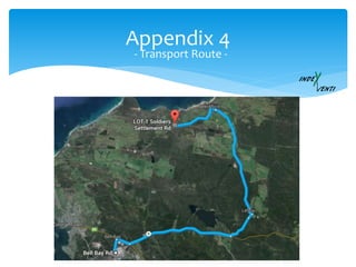
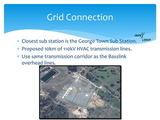
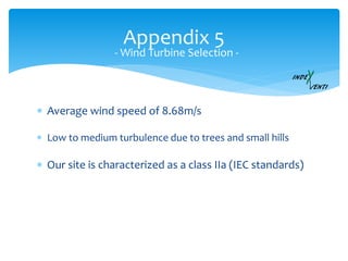
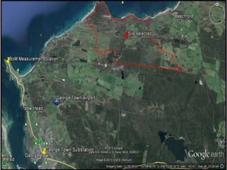
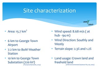
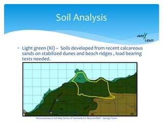
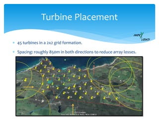
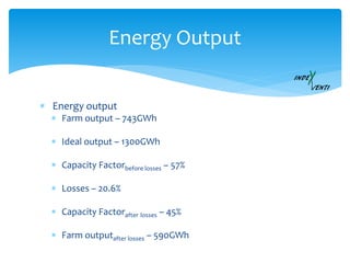
This document provides a feasibility study for the proposed Low Head Wind Farm in Tasmania. Key points include: 1) The site was chosen for its strong and consistent wind resource as well as proximity to transmission infrastructure. 2) Wind resource analysis was conducted using on-site and nearby weather station data, showing average wind speeds of 8.68 m/s suitable for wind power generation. 3) The project would involve installing 45 turbines with a total capacity of 148.5 MW, generating an estimated 590 GWh annually after losses. 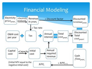4) Financial modeling under high, medium, and low electricity price scenarios showed the project would be economically viable with a medium price of $90/MWh, yielding

1. Low Head Wind Farm
Ankit Grover
Byoungmo Kang
Cecilia M. Ferreira
Liang Zhao
Feasibility study

2.  Tasmania has a great wind resource known as the
roaring forties.
Why investing in a Tasmanian wind
farm is a good idea?
 Two-thirds of Tasmanian
electricity generation comes from
Hydro-electricity. There is a need
for balance!
 Use the Basslink to sell electricity to
the mainland when demand is high.
Office of the Economic Regulator, 2014

4. Site characterization
• Area: 15.7 km
2
• 6 km to George Town
Airport
• 7.2 km to BoM Weather
Station
• 10 km to George Town
Substation (220 kV)
• Wind speed: 8.68 m/s ( at
hub - 94 m)
• Wind Direction: Southly and
Westly
• Terrain slope: 2.3% and 1.2%
• Land usage: Crown land and
freehold land
(SFM Environmental Solutions Pty Ltd, 2005)(Transend Networks, 2014)

5. Wind Resource Analysis
• Low Head Station
- Speed and Distribution -
• Gradient Height 250 m
• Surface Roughness: 30 mm
(Robertson & Gaylord, 1980)

6. Wind Resource Analysis
• Selected Site
- Speed and Distribution -
• Gradient Height 400 m
• Surface Roughness: 700 mm
(Robertson & Gaylord, 1980)

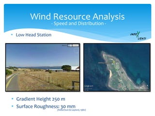
7. Wind Resource Analysis
- Speed and Distribution -
Height
[m]
Surface
roughness
[m]
Gradient
height
[m]
Mean
wind
speed
[m/s]
Standard
deviation
BoM
Station
10 0.03 250 7.24 3.036
Wind farm
site
94 0.70 400 8.68 3.642
• IEC 61400 – 1 : Wind class II

8. Wind Resource Analysis
- Speed and Distribution -
0%
2%
4%
6%
8%
10%
12%
14%
0 1 2 3 4 5 6 7 8 9 10 11 12 13 14 15 16 17 18 19 20 21 22 23 24 25 26 27 28 29 30
Probability[m/s]
Wind speed [m/s]
Weibull PDF
Actual data

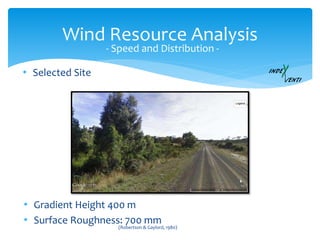
9. Wind Resource Analysis
- Speed and Distribution -
0
5
10
15
20
25
30
0 1000 2000 3000 4000 5000 6000 7000 8000 9000
Windspeed[m/s]
Duration [hours]
Velocity-duration chart

10. Wind Resource Analysis
- Directionality -

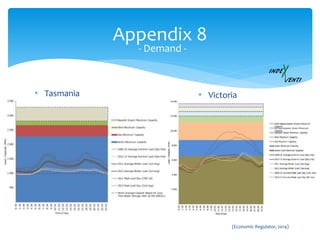
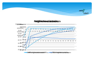
11. Wind Resource Analysis
- Correlation with demand -
0
10
20
30
40
50
60
0
200
400
600
800
1000
1200
1400
0:00 4:48 9:36 14:24 19:12 0:00
Electricitygenerated[MWh]
Demand[MWh]
Time of day
Daily summer profile
TAS Demand Wind farm output
0
10
20
30
40
50
60
0
200
400
600
800
1000
1200
1400
1600
0:00 4:48 9:36 14:24 19:12 0:00
Electricitygenerated[MWh]
Demand[MWh]
Time of day
Daily winter profile
TAS Demand Wind farm output
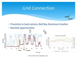
• Demand data from AEMO
(Australian Energy Market Operator, 2015)
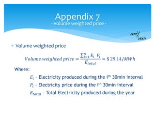
𝑉𝑜𝑙𝑢𝑚𝑒 𝑤𝑒𝑖𝑔ℎ𝑡𝑒𝑑 𝑝𝑟𝑖𝑐𝑒 = $ 29.14/𝑀𝑊ℎ

12. Wind Turbine Selection
Using this Information we
selected the:
VESTAS V112 3.3MW
Vestas Online

13. Turbine Placement
8D
8D
 Spacing: roughly 850m in both directions to reduce array losses.
 45 turbines in a 2x2 grid formation.

14. Energy Output
 Energy output
 Farm output – 743GWh
 Ideal output – 1300GWh
 Capacity Factorbefore losses – 57%
 Losses – 20.6%
 Capacity Factorafter losses – 45%
 Farm outputafter losses – 590GWh

15. Construction

16.  Sea Transport
Transportation
Vestas V112 - Macarthur wind farm
 Port of Bell Bay is 27km from wind farm site.
 Deep Waters in the Tamar River.
 Current crane tonnage – 19tonnes, will need to be
increased.
 Road Transport
 3 temporary roadblocks will
need to be set.
 3 difficult left turns to
maneuver.
 Soldiers Settlement road.

17. Soil Analysis
 Light green (Kl) – Soils developed from recent calcareous
sands on stabilized dunes and beach ridges , load bearing
tests needed.
Reconnaissance Soil Map Series of Tasmania For Beaconsfield – George Town

18.  Closest sub station is the George Town Sub Station.
 Proposed 10km of 110kV HVAC transmission lines.
 Use same transmission corridor as the Basslink
overhead lines.
Grid Connection

19.  Proximity to load centers, Bell Bay Aluminum Smelter
 Basslink opportunities
Grid Connection
Office of the Economic Regulator, 2014

20. Avian Fauna
Land clearance
Waste management
Environmental impact

21. Avian Fauna
https://thewindenergysolution.wordpress.com/4-concessionrefutation/

22.  According to Dr. Cindy Hall number of collisions
decreasing in Tasmania
 Most common : Brown Thornbill and Silver Gull
Avian Fauna

23.  Site is composed with free
hold land and crown land
owned by the
government. (The Crown)
 Can be bought or Leased
 Small amount of Land
clearance required
Land
(SFM Environmental Solutions Pty Ltd, 2005)

24.  Possible waste
produced from
construction
 No harmful or
hazardous waste during
operation
 Cleanest energy source
 Disposal of wind turbine
after lifespan
 Recycle in thermal and
mechanical uses
Waste management
http://www.holcim.com/en/referenceprojects/disused-rotor-blades-can-now-
be-utilized-in-cement-production.html

25.  Visual Impact
 Noise Impact
 Local and government opinions
Social Impact

26. Social Impact

27.  Located near coastline –
Possible destructive coastal
view
 Distance from housings are far
enough
 No SHADOW FLICKER (Range
of 550m)
 Wind turbines are recognized
as symbol of renewable
energy
Visual Impact

28.  Wind farm noise – the biggest problem for local
residents
 Noise level of wind farm 103 dB
 Allowed noise level 35 dB at housing
 Presence of trees and direction of wind blowing away
from the housing
Noise Impact

29.  Tasmanian government-the premier Will Hodgman
"Tasmania as a renewable energy state has
tremendous capacity, I believe, into the future”
 Previous wind farms in TAS were supported by local
communities
 Employment and local business development
 Possible opposition group (NIMBY)
Opinions

30. Financial Modeling
Electricity
𝑝𝑟𝑖𝑐𝑒 𝑦𝑒𝑎𝑟𝑖
Revenue
in 𝑦𝑒𝑎𝑟𝑖
Discounted
𝑟𝑒𝑣𝑒𝑛𝑢𝑒 𝑦𝑒𝑎𝑟𝑖
O&M cost
per year
Annual
interest
Total
𝑐𝑜𝑠𝑡 𝑦𝑒𝑎𝑟𝑖
Discounted
Total
𝑐𝑜𝑠𝑡 𝑦𝑒𝑎𝑟𝑖
Initial
cost
Tax
Capital
cost
Annual
required
revenue
×Electricity
produced
× Discount factor
× Tax rate
DF
×Capacity
Cash
𝑓𝑙𝑜𝑤 𝑦𝑒𝑎𝑟𝑖
𝑁𝑃𝑉𝑖
+ 𝑁𝑃𝑉𝑖−1
(Initial NPV equal to the
negative initial cost)

31. High revenue
scenario
Medium revenue
scenario
Low revenue
scenario
Capital costs (million
AU$/MV)
1.7 2.35 2.53
Life time (years) 20 20 20
Discount rate 10% 10% 10%
Inflation rate 0.024 0.024 0.024
Construction time
(years)
1 1 2
Total O&M per year
($/MW)
10297682.74 10297682.74 10297682.74
Electricity price
(AU$/MWh)
110.00 90.00 39.056(in 2017)
Capacity factor 45.38% 45.38% 45.38%
O&M Cost $10297682.74 $10297682.74 $10297682.74
Tax rate 0.03 0.03 0.03
NPV of project $308002166.50 $61451272.20 -$97643477.50
IRR 25.34% 12.95% 7.58%
LCE(AU$/MWh) 60.81288773 77.0976962 81.60733547

32. -3E+08
-2E+08
-1E+08
0
100000000
200000000
300000000
400000000
1 2 3 4 5 6 7 8 9 10 11 12 13 14 15 16 17 18 19 20 21
High Revenue Scenario
NPV in high revenue scenario Cashflow in high revenue scenario
-7E+08
-6E+08
-5E+08
-4E+08
-3E+08
-2E+08
-1E+08
0
100000000
1 2 3 4 5 6 7 8 9 10 11 12 13 14 15 16 17 18 19 20 21 22
Low Revenue Scenario
Cashflow in low revenue scenario" NPV in low revenue scenario
-8E+08
-7E+08
-6E+08
-5E+08
-4E+08
-3E+08
-2E+08
-1E+08
0
100000000
200000000
1 2 3 4 5 6 7 8 9 10 11 12 13 14 15 16 17 18 19 20 21
Medium Revenue Scenario
Cashflow in medium revenue scenario NPV in medium revenue scenario

33. Conclusion
 Main advantages:
 Strong wind resource
 Good correlation with demand and possibility to sell to Victorian market
 Proximity to a port, a substation as well as to a load center
 Existence of a road connecting the site
 What is necessary to move forward with the project:
 Do wind measurements at the site to substitute the use of projected
data
 Do soil and geography analysis to choose the foundation type
 Do further fauna assessments (as this is a site specific issue)
 Study the effect of blade glint on road users
 Check the availability of the Crown Land and if the other landlords will
be willing to lease their land

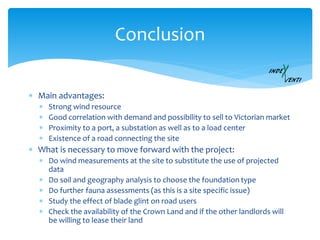
34. Conclusion
The construction of a 148.5 MW wind farm will be able to generate
590 [GWh] per year.
However, It will be necessary to do a Power Purchase Agreement to
make the project financially viable. Therefore it became an interesting
investment with:
Medium revenue ($90/MWh)
 NPV: $ 61,451,272.20
 IRR: 12.95%
 SPB: 12 years
High revenue ($110/MWh)
 NPV: $ 308,002,166.50
 IRR: 25.34%
 SPB: 7 years

35. The Low Head Wind Farm is the right
Choice!

36. References
Australian Energy Market Operator. (2015). Aggregated Price and Demand Data Files. Retrieved April 25, 2015, from
http://www.aemo.com.au/Electricity/Data/Price-and-Demand/Aggregated-Price-and-Demand-Data-Files
Economic Regulator. (2014, February). Energy in Tasmania - Performance Report 2012-13. Retrieved April 30, 2015, from
http://www.economicregulator.tas.gov.au/domino/otter.nsf/LookupFiles/Energy_in_Tasmania_Performance_Report_2012-
13_FINAL_140212.pdf/$file/ Energy_in_Tasmania_Performance_Report_2012-13_FINAL_140212.pdf
Robertson, L. E., & Gaylord, E. H. (1980). Section 3.3.2 - Properties of the Mean Wind. In Tall building: criteria and loading (pp.
161 - 162). New York: American Society of Civil Engineers.
SFM Environmental Solutions Pty Ltd. (2005, October). George Town Coastal Management Plan. Retrieved April 7, 2015, from
http://georgetown.tas.gov.au/coastal-reserve-management-lan?fd=pP%25F8%25F0%252F%25B5%25E7%25D
D%25A3%25EDJ%2588%25B4r%25FC%25F6d%25DC%25CEO%252FI%253A%253FN5D%25CD%25F3%252FMA26%253F
Transend Networks. (2014, June 30). Annual Planning Report: 2014. Retrieved April 1, 2015, from
http://www.tasnetworks.com.au/TasNetworks/media/pdf/Transend-Annual-Planning-Report-2014.pdf
Office of the Tasmanian Economic Regulator. (2014). Energy in Tasmania - Performance Report 2012/13.
Department of Primary Industries, Parks, Water and Environment. RECONNAISSANCE SOIL MAP SERIES OF TASMANIA
BEACONSFIELD-GEORGE TOWN.

37. Appendix 1
- OLS of George Town Airport -

38. Appendix 2
In order to translate the wind measurements from the BoM station to hub height at the
proposed wind farm site, firstly, it is necessary to calculate the free stream speed,𝑈 𝐹𝑆, at the
BoM station from its measured wind velocity, 𝑈𝑠𝑡𝑎𝑡𝑖𝑜𝑛. Using the logarithmic law, this can be
done with the following equation:
𝑈 𝐹𝑆 = 𝑈𝑠𝑡𝑎𝑖𝑜𝑛
ln
𝑧 𝑔𝑟𝑎𝑑−𝑠𝑡𝑎𝑡𝑖𝑜𝑛
𝑧0−𝑠𝑡𝑎𝑡𝑖𝑜𝑛
ln
𝑧𝑠𝑡𝑎𝑡𝑖𝑜𝑛
𝑧0−𝑠𝑡𝑎𝑡𝑖𝑜𝑛
As it is reasonable to assume that the free stream speed is the same in both sites, it is
possible to scale down the wind speed from gradient to hub height at the wind farm site,
𝑈𝑆𝑖𝑡𝑒, using again the logarithmic law:
𝑈𝑆𝑖𝑡𝑒 = 𝑈 𝐹𝑆
ln
𝑧ℎ𝑢𝑏
𝑧0−𝑠𝑖𝑡𝑒
ln
𝑧 𝑔𝑟𝑎𝑑−𝑠𝑖𝑡𝑒
𝑧0−𝑠𝑖𝑡𝑒
- Scaling Wind Speeds -

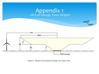
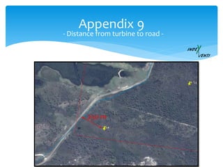
39. Appendix 3
The Weibull distribution is used to approximate the distribution of wind speeds for a certain location. It uses two
parameters: k, called shape factor, and c, called scale factor. Which can be calculated using the mean wind speed, 𝑈,
and the standard deviation, σ, of a dataset with the following equations:
𝑘 =
σ
𝑈
−1.086
𝑐 = 𝑈 0.568 +
0.433
𝑘
−1/𝑘
With this parameters, it is possible to calculate the Weibull Probability Density Function (PDF) which is
the relative likelihood in [m/s] of having wind at speeds of U [m/s]:
𝑃𝐷𝐹 𝑈 =
𝑘
𝑐
𝑈
𝑐
𝑘−1
𝑒
−
𝑈
𝑐
𝑘
And the Weibull Cumulative Distribution Fuction (CDF) which is the probability of having wind speeds
below U [m/s]:
𝐶𝐷𝐹 𝑈 = 1 − 𝑒
−
𝑈
𝑐
𝑘
Therefore, it is possible to calculate the probability of finding wind speed within a range of velocities
by:
𝑈1 < 𝑈 < 𝑈2 = 𝐶𝐷𝐹 𝑈2 − 𝐶𝐷𝐹 𝑈1
This can be used to calculate the number of hours per year that the wind blows within that range of
speeds and the energy output. (Manwell, McGowan, & Rogers, 2004)
- Weilbul Distribution -

40. Appendix 4
- Transport Route -

41. Appendix 5
- Wind Turbine Selection -
 Our site is characterized as a class IIa (IEC standards)
 Low to medium turbulence due to trees and small hills
 Average wind speed of 8.68m/s

42. Appendix 6
- Losses -
 Losses –
 Array Losses – 13% (Katics Model)
 Electrical Efficiency Losses – 4% (Informed assumption)
 Soiling losses – 2% (informed assumption)
 Machine downtime losses – 2% (informed assumption)
 Other losses – 1%, e.g wind direction hysteresis (informed
assumption)
 Total loss percentage – 20.6%

43. Appendix 7
 Volume weighted price
- Volume weighted price -
𝑉𝑜𝑙𝑢𝑚𝑒 𝑤𝑒𝑖𝑔ℎ𝑡𝑒𝑑 𝑝𝑟𝑖𝑐𝑒 =
𝑖=1
𝑛
𝐸𝑖 𝑃𝑖
𝐸𝑡𝑜𝑡𝑎𝑙
= $ 29.14/𝑀𝑊ℎ
Where:
𝐸𝑖 – Electricity produced during the ith 30min interval
𝑃𝑖 – Electricity price during the ith 30min interval
𝐸𝑡𝑜𝑡𝑎𝑙 – Total Electricity produced during the year

44. Appendix 8
- Demand -
• Tasmania • Victoria
(Economic Regulator, 2014)

45. Appendix 9
- Distance from turbine to road -
250 m

46. Appendix 10
 Initial cost:
𝑐𝑜𝑠𝑡𝑠𝑖𝑛𝑖𝑡𝑖𝑎𝑙 = 𝑐𝑎𝑝𝑖𝑡𝑎𝑙 𝑐𝑜𝑠𝑡 $𝑝𝑒𝑟 𝑀𝑊 × 𝑝𝑙𝑎𝑛𝑡 𝑟𝑎𝑡𝑒𝑑 𝑝𝑜𝑤𝑒𝑟 𝑀𝑊
 The O&M cost could calculate by:
O&M 𝑒𝑞𝑢𝑖𝑣𝑎𝑙𝑒𝑛𝑡,𝑓𝑖𝑥𝑒𝑑= 𝑂&𝑀𝑣𝑎𝑟𝑖𝑎𝑏𝑙𝑒×C × 8760
𝐻𝑂𝑈𝑅𝑆
𝑌𝐸𝐴𝑅
(NOTE, C is
the capacity factor.)
O&M cost per year = O&M 𝑒𝑞𝑢𝑖𝑣𝑎𝑙𝑒𝑛𝑡,𝑓𝑖𝑥𝑒𝑑 + 𝑂&𝑀𝑓𝑖𝑥𝑒𝑑
 Calculation of𝐀𝐧𝐧𝐮𝐚𝐥 𝐢𝐧𝐭𝐞𝐫𝐞𝐬𝐭:
PV=A×
1−(
1+𝑖
1+𝑓
)−𝑁
1+𝑖
1+𝑓
, PV= the initial cost; A is annual required revenue
A= PV/
1−(
1+𝑖
1+𝑓
)−𝑁
1+𝑖
1+𝑓
→ Annual interest=
n×𝐴−𝑐𝑜𝑠𝑡𝑠 𝑖𝑛𝑖𝑡𝑖𝑎𝑙
𝑛
- Financial Modeling -

47.  Discount Factor : (
1+𝑖
1+𝑓
)−𝑁
𝑇𝑎𝑥𝑖 = revenue𝑖 × 0.03
 𝑵𝑷𝑽𝒊= 𝑁𝑃𝑉𝑖−1 +Discounted revenue𝑖 − The discounted total
𝑐𝑜𝑠𝑡 𝑦𝑒𝑎𝑟𝑖
(Initial NPV equal to the negative initial cost)
 Levelised cost of electricity is calculated by:
LCOE=
Annual required revenue
𝐴𝑛𝑛𝑢𝑎𝑙 𝐸𝑛𝑒𝑟𝑔𝑦 𝑃𝑟𝑜𝑑𝑢𝑐𝑡𝑖𝑜𝑛
+
O&M 𝑒𝑞𝑢𝑖𝑣𝑎𝑙𝑒𝑛𝑡,𝑓𝑖𝑥𝑒𝑑+𝑂&𝑀 𝑓𝑖𝑥𝑒𝑑
𝑛𝑛𝑢𝑎𝑙 𝐸𝑛𝑒𝑟𝑔𝑦 𝑃𝑟𝑜𝑑𝑢𝑐𝑡𝑖𝑜𝑛

48. • BoM Weather Station: Low Head Lighthouse
• Datasets:
 Hourly wind data from 6 June 2000 to 16 February 2011
 And half-hourly wind measurements from 1 January 2011 to
4 July 2012.
Appendix 11
- Wind data -