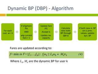
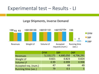
The document explores bid-price heuristics for cargo revenue management, emphasizing the shift from restriction/class-based to willingness-to-pay-based pricing strategies. The study tests various algorithms, including static and dynamic bid-price approaches, to optimize revenue under uncertain capacity conditions. Results indicate that the willingness-to-pay model enhances revenue effectiveness and suggests areas for future research and policy improvement.

1. BID-­‐PRICE
HEURISTICS
FOR
UNRESTRICTED
FARE
STRUCTURES
IN
CARGO
REVENUE
MANAGEMENT
L.
Castelli
1,
R.
Pesen@
2,
D.
Rigonat
1
1
Università
degli
Studi
di
Trieste,
Italy
2
Università
Ca’Foscari,
Venezia,
Italy

2. Revenue
Management
&
Cargo
A
collec'on
of
pricing,
inventory,
marke'ng
techniques
aimed
at
predic'ng
consumer
behaviour
and
op'mize
product
availability
and
price
to
maximize
revenue
growth.
In
cargo:
¨ Total
available
capacity
(=
product
inventory)
may
be
uncertain;
¨ Bi-­‐dimensional
capacity
(weight,
volume);
¨ Tri-­‐dimensional
alloca@on;
¨ Product
value
increases
over
@me
then
drops
to
zero.

3. Product-­‐oriented
vs.
Price-­‐oriented
Demand
RM
forecasts
shiY
from
restric@on/class-­‐based
to
willingness
to
pay
(wtp)-­‐based
Product-­‐oriented
Price-­‐oriented
Different
fares
for
different
products
A
single
type
of
product
Customer
only
interested
in
a
specific
fare/product
Customer
purchase
solely
on
price
Customer
choice
independent
of
the
availability
of
cheaper
services
Customer
compare
services
from
different
carriers
to
get
the
cheapest
fare

4. Objec@ve
of
our
study
¨ Study
effec@veness
of
capacity
management
algorithms
based
on
willingness
to
pay;
¨ Develop
policies
that
are
suitable
for
cargo
context;
¨ Explore
different
approaches:
¤ Dynamic
Programming
(DP)
¤ Bid-­‐Prices
(BP)

5. Roadmap
Defini@on
of
the
scenario
General
problem
formula@on
through
Dynamic
Programming
(DP)
DP
based
algorithm
Bid-­‐price
(BP)
approach:
sta@c
BP
(SBP)
and
dynamic
BP
(DBP)
algorithms
Tests
on
different
shipment
size
/customer
demand
combina@on

6. Problem
formula@on
-­‐
Assump@ons
¨ Cargo
scenario
(i.e.
air
cargo):
bi-­‐dimensional
capacity
(weight,
volume);
¨ 3-­‐D
alloca@on
issues
are
ignored;
¨ Single
class
of
customers;
¨ Customers
are
served
one
at
a
@me
(1
customer
=
1
shipment);
¨ A
shipment
can
be
accepted
only
if
the
flight
has
residual
capacity
(volume
and
weight)
to
accommodate
it;
¨ A
shipment
is
paid
for
propor@onally
to
its
weight
(revenue
=
weight
*
unitFare).

7. Problem
formula@on
-­‐
Nota@on
Symbol
Meaning
F={f1,…,fM} Set
of
increasing
fares
f ∈ F Generic
fare
pkm Willingness
of
k-­‐th
customer
to
pay
fare
m
{0,1,…,t,t+1,…,T} Time
frame
from
reserva@on
opening
to
closure
tk ∈ {0,…,T} Generic
@me
instant
φt probability
of
a
customer
showing
up
at
@me
t
Cw , Cv AircraY
capacity
for
weight,
volume
(w,v) Residual
aircraY
capacity
for
weight,
volume
(ω,υ) Shipment
size
qωυ Probability
that
a
shipment
has
size
(w,u)
Jm(t,w,v) Func@on
that
returns
the
expected
op@mal
revenues
from
@me
t
onwards
assuming
fare
fm
is
displayed
and
there
are
residual
capaci@es
(w,v).

8. Problem
formula@on
(DP)
At
@me
T
No
customer
arrives
Revenues
in
T=
revenues
in
T+1
A
customer
arrives
Shipment
does
not
fit
Revenues
in
T=
revenues
in
T+1
Shipment
fits
We
offer
fare
f
Customer
refuses
f
Revenues
in
T=
revenues
in
T+1
Customer
accepts
f
Shipm.
accepted
Rev
=
f*w
Cap.
w,v
updated
We
offer
fare
f+1
Calculate
recursion
for
f+1

9. DP
algorithm
(DYM)
Assuming
that
n.
of
customers,
arrival
@mes,
willingness
to
pay
and
shipment
sizes
are
known
in
advance,
DP
is
simplified
into
(2).
Jm(k,w,v) = maxj≥m{ pkj (fjω + Jj(k+1,w-ω,v-υ)) + (1- pkj)Jj(k+1,w,v)} (2)
with final conditions
Jm(k,0,v)= Jm(k,w,0)= Jm(K+1,w,v) = 0 for all 0 ≤ w ≤ Cw and 0 ≤ v ≤ Cv and k ≤ K
For
each
cust.
arrival
k
If
shipment
fits
Calculate
(2)
for
all
fares
≥
m
Check
final
condi@ons
Hence
the
algorithm:

10. Bid-­‐price
approach
-­‐I
Jm(t,w,v) – Jm(t,w-ω,v-υ)
Represents
the
opportunity
cost
at
fare fm for
a
shipment
of
size
(ω,υ) appearing
at
@me t when
capaci@es w,v are
s@ll
available.
Expected
loss
in
future
revenue
from
using
the
capacity
now
rather
than
reserving
it
for
future
use;
An
op@mal
policy,
solu@on
of
DP,
accepts
a
shipment
iff
generated
revenues
are
≥ to
its
opportunity
cost.

11. Bid-­‐price
approach
-­‐
II
If Jm(t,w,v) is
differen@able
then
∂Jm(t,w,v)/∂w and
∂Jm(t,w,v)/∂v are
the
weight
marginal
opportunity
cost
and
volume
marginal
opportunity
cost,
respec@vely.
We
can
calculate
an
approxima@on
of
the
marginal
opportunity
cost
(a
bid-­‐price)
We
can
design
policies
that
accept
a
shipment
only
when
its
revenue
is
≥ to
the
es@ma@on
of
the
opportunity
cost
obtained
through
the
BP

12. Bid-­‐price
approach
-­‐
III
Formally,
the
acceptance
rule
for
a
BP
policy
is:
Symbol
Meaning
r Shipment
revenue
πw(w,t) , πv(v,t) Weight
and
volume
BP
πw(w,t)ω + πv(v,t)υ Opportunity
cost
f Applied
fare
r = fω ≥ πw(w,t)ω + πv(v,t)υ (3)

13. ¨ Sta'c
BP:
fixed
at
the
beginning
of
the
booking
period
i.e.,
they
do
not
change
over
@me
and
do
not
depend
on
the
remaining
capacity:
πw(w,t) = πw , πv(v,t) = πv.
¨ The
chosen
fare
is
unique
for
all
customers:
i.e.
the
min
f s.t.
rule
(3)
is
respected
by
1st
accepted
customer:
f = min{fj : fjωh ≥ πwωh + πvυh and phj = 1}
Sta@c
BP
Algorithm
(SBP)
-­‐
I

14. Sta@c
BP
Algorithm
(SBP)
-­‐
II
Calculates
op@mal
BP
for
each
instance
from
a
training
set.
Training
Phase
SBP-­‐A
Tes@ng
Phase
SBP-­‐B
Checks
acceptance
rule
(3)
with
avg.
op@mal
BP
(πw
, πv)
obtained
from
training
alg.
Op@mal
BP
per
instance
πw
, πv

15. Dynamic
BP
(DBP)
Limita@ons
of
SBP:
¨ Revenue
depends
on
willingness
to
pay
of
the
first
accepted
customer:
bad
for
inverse
demand;
¨ BP
do
not
change
over
@me
but
residual
capacity
value
increases
over
@me.
Idea
behind
DBP:
¨ Dynamic
BP
are
updated
aYer
each
accepted
customer
by
running
SBP-­‐A
on
the
residual
capacity;
¨ Fares
are
updated
based
on
both
users’
wtp
and
dyn.
BP
update.

16. Dynamic
BP
(DBP)
-­‐
Algorithm
For
each
cust.
arr.
k
If
shipment
fits
AND
wtp
current
fare
=
1
Update
fare
(4);
Accept
k;
Update
res.
capacity
Calculate
new
sta@c
BP
through
SBP-­‐A
If
both
new
st.
BP
are
≥
prev.
values,
update
dyn.
BP
f= min in F={f1,…,fM}: fjωk ≥ Lkωk + Mkυk (4)
Fares
are
updated
according
to:
Where
Lk,
Mk
are
the
dynamic
BP
for
user
k

17. Experimental
test
-­‐
Setup
¨ Small
shipments
(SS):
n
=
750;
between
2
and
45
Kg
¨ Large
shipments
(LS):
n=
450;
between
46
and
500
Kg
¨ Inverse
Demand
(ID):
wtp
decreases
with
customer
arrivals
¨ Random
Demand
(RD):
random
wtp
SS-ID SS-RD
LS-ID LS-RD
Test
Scenarios:

18. Experimental
test
–
Results
-­‐
SR
85 85 85 85
113100 100 100 100 10093 96 97 93
0
Revenues
Weight
LF
Volume
LF
Accepted
requests
(num.)
Running
@me
(sec.)
DYM
SBP
DBP
DYM
SBP
DBP
Revenues
2,458,003
2,283,183
2,082,226
Weight
LF
0.999
0.964
0.849
Volume
LF
0.869
0.839
0.738
Accepted
req.
(num.)
178
166
152
Running
@me
(sec.)
552
0.5
624
Small
Shipments,
Random
Demand

19. Experimental
test
–
Results
-­‐
LR
100 100 100 100 10098 100 99 96
1
93 94 94 94
3
Revenues
Weight
LF
Volume
LF
Accepted
requests
(num.)
Running
@me
(sec.)
DYM
SBP
DBP
DYM
SBP
DBP
Revenues
4,752,162
4,641,544
4,421,279
Weight
LF
0.82
0.816
0.77
Volume
LF
0.997
0.992
0.935
Accepted
req.
(num.)
51
49
48
Running
@me
(sec.)
64
0.5
2
Large
Shipments,
Random
Demand

20. Experimental
test
–
Results
-­‐
SI
100 100 100 100 100
76
100 100 101
0
78
100 100 102
21
Revenues
Weight
LF
Volume
LF
Accepted
requests
(num.)
Running
@me
(sec.)
DYM
SBP
DBP
DYM
SBP
DBP
Revenues
2,712,138
2,053,969
2,121,717
Weight
LF
0.999
1
1
Volume
LF
0.87
0.87
0.87
Accepted
req.
(num.)
171
173
174
Running
@me
(sec.)
594
0.5
122
Small
Shipments,
Inverse
Demand

21. Experimental
test
–
Results
-­‐
LI
100 100 100 100 10092 100 101 102
1
93 100 101 104
6
Revenues
Weight
LF
Volume
LF
Accepted
requests
(num.)
Running
@me
(sec.)
DYM
SBP
DBP
DYM
SBP
DBP
Revenues
5,110,171
4,680,050
4,736,291
Weight
LF
0.821
0.823
0.824
Volume
LF
0.99
0.999
0.998
Accepted
req.
(num.)
47
48
49
Running
@me
(sec.)
79
0.5
5
Large
Shipments,
Inverse
Demand

22. Where
we
go
from
here..
We
proved
the
reliability
of
wtp-­‐based
policies
within
the
defined
scenario
(determinis@c
demand,
weight-­‐based
pricing
etc.)
Future
work:
¨ Improvement
to
the
proposed
policies
¨ Comparison
with
policies
developed
by
other
authors