Download to read offline


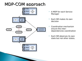
![ C=SxA -->|R
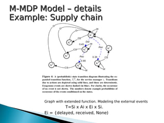
Cost function: Cost of invocation + cost of
waiting for delayed order + cost of
changing supplier
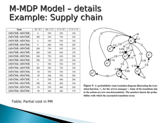
OC: optimal criterion.
Horizon= Expected cost over finite steps.
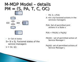
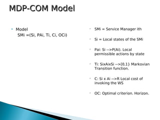
M-MDP Model – detailsM-MDP Model – details
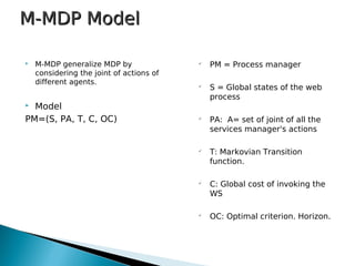
PM = (S, PA, T, C, OC)PM = (S, PA, T, C, OC)
T = SxAxS --> [0,1]. Markovian
transition function
Captures the global effect of
jointly invoking WS by SM
T(s'|s,a) = T[(s'i, s'j) | (si, sj),(ai, aj)]
...
T(s'|s,a)= Ti[s'i | (si, ai)] * Tj[s'j, (sj,aj)]
Ti and Tj individual transition functions
This is possible because each service
manager's next state is influenced
only by its own action and its current
state.](https://image.slidesharecdn.com/optimaladaptationautonomicwsinterservicesdepenecies-101027120242-phpapp02/85/Optimal-Adaptation-16-320.jpg)
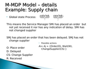


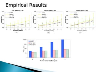


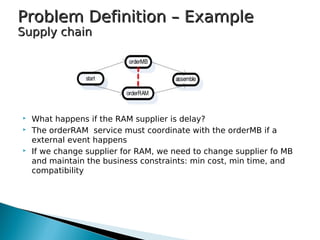
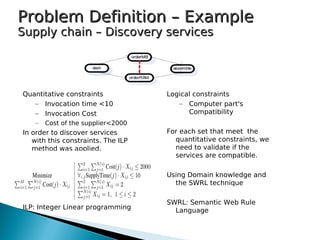
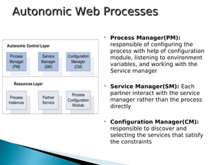
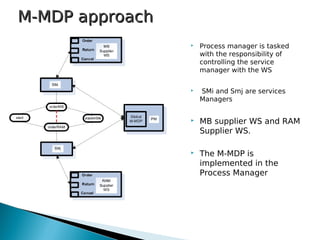
1) The document presents frameworks for optimal adaptation in autonomic web processes that have inter-service dependencies. It describes two approaches: M-MDP which uses a centralized Markov decision process and MDP-COM which uses a decentralized approach with local Markov decision processes and a coordination mechanism. 2) The supply chain example involves ordering computer parts from suppliers, with the goal of minimizing costs and response times while maintaining compatibility between parts. External events like delivery delays require adaptation. 3) The approaches were tested on a supply chain process implemented in METEOR-S, comparing performance under different horizons, event probabilities, and numbers of service managers. A hybrid model combining aspects of both approaches was also explored.