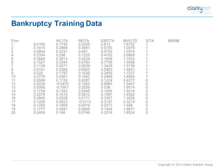
Download as PDF, PPTX


![Copyright © 2012 Clarity Solution Group
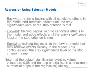
Logisitic regression
p = Prob(y=1|x) = exp(a+bx)/[1+exp(a+bx)]
1-p =1/[1+exp(a+bx)]
ln [p/(1-p)] = a + bx
where:
exp ore is the exponential function(e=2.71828…)
lnis the natural logarithm (ln(e) = 1)
p is probability that the event y occurs given x, and can range between 0 and 1
p/(1-p) is the "odds ratio"
ln[p/(1-p)] is the log odds ratio, or "logit"
all other components of the regression model are the same](https://image.slidesharecdn.com/558790d2-2a1f-4e5e-af99-d63a58c9b8c3-141124185521-conversion-gate01/85/Predictive-Modeling-with-Enterprise-Miner-44-320.jpg)
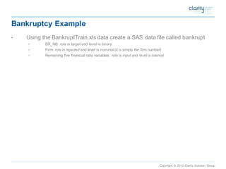
![Copyright © 2012 Clarity Solution Group
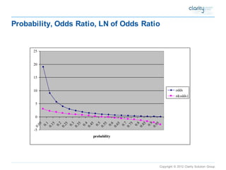
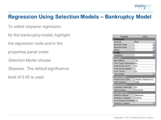
Odds Ratio
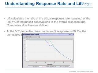
•Frequently used
•Related to probability of an event as follows: Odds Ratio = p/(1-p)
•Example:
•Probability of firm going bankrupt = .25
•Odds firm will go bankrupt = .25/(1-.25) = 1/3 or 3 to 1
•This is how sports books calculate odds
•(e.g., if odds of VU winning a championship are 2:1, probability is 1/3
•ln [p/(1-p)] = a + bx means that as x increases by 1, the natural log of the odds ratio increases by b, or the odds ratio increase by a factor of exp(b)](https://image.slidesharecdn.com/558790d2-2a1f-4e5e-af99-d63a58c9b8c3-141124185521-conversion-gate01/85/Predictive-Modeling-with-Enterprise-Miner-45-320.jpg)
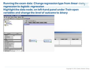
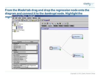
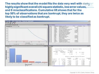
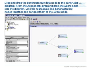
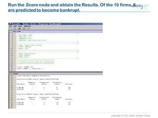
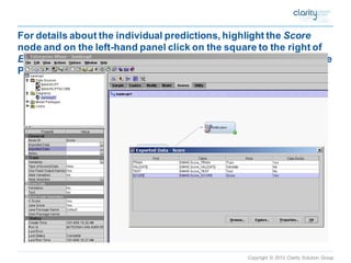
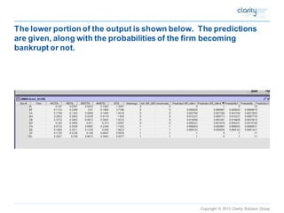

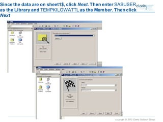
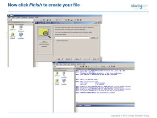
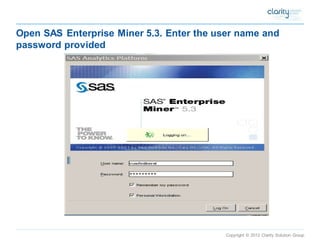
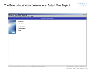
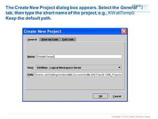
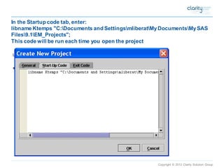
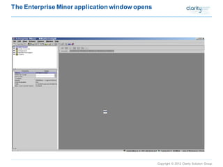
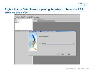
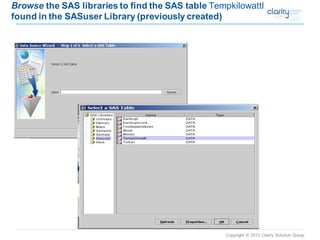
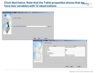
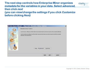
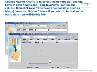
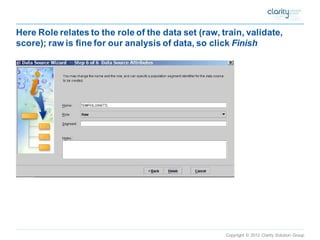
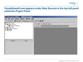
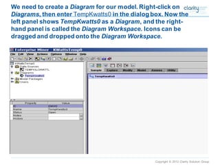
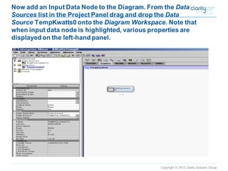
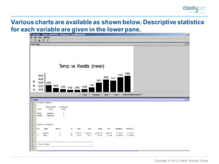
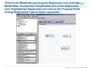
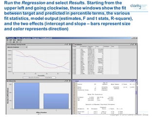
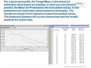
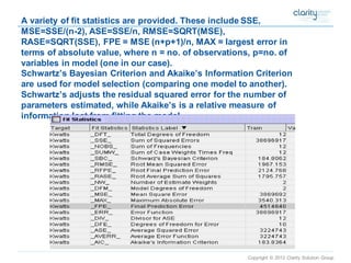
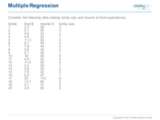
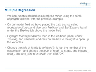
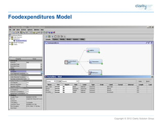
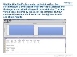
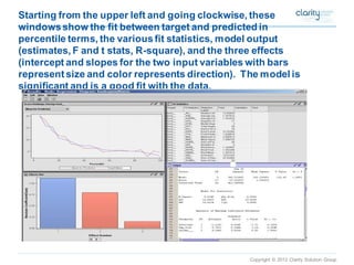
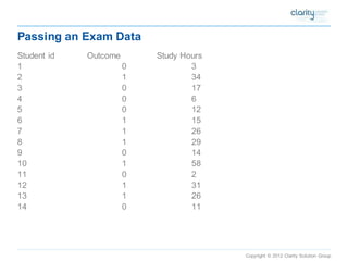
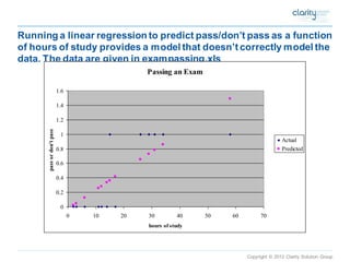
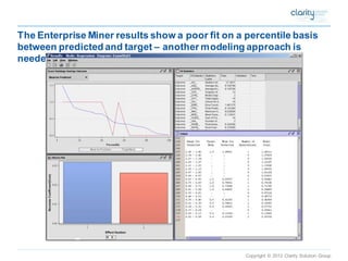
This document provides an overview of using SAS Enterprise Miner software to conduct predictive modeling using regression analysis. It discusses how to import data from Excel, create a project and data source in Enterprise Miner, run linear and logistic regression models to predict outcomes, and interpret the results, including measures of model fit and variable effects. Examples are provided demonstrating linear regression of kilowatt usage on temperature, multiple regression of food expenditures on income and family size, and logistic regression of exam passing on study hours.