Predicting anomalies in computer networks using autoencoder based representation learning

International Journal of Informatics and Communication Technology (IJ-ICT)
Vol. 13, No. 1, April 2024, pp. 9~26
ISSN: 2252-8776, DOI: 10.11591/ijict.v13i1.pp9-26  9
Journal homepage: http://ijict.iaescore.com
Predicting anomalies in computer networks using autoencoder-
based representation learning
Shehram Sikander Khan1
, Akalanka Bandara Mailewa2
1
Department of Information Assurance, St. Cloud State University, St. Cloud, USA
2
Department of Computer Science and Information Technology, St. Cloud State University, St. Cloud, USA
Article Info ABSTRACT
Article history:
Received Dec 21, 2021
Revised Jan 3, 2023
Accepted Jun 13, 2023
Recent improvements in the internet of things (IoT), cloud services, and
network data variety have increased the demand for complex anomaly
detection algorithms in network intrusion detection systems (IDSs) capable
of dealing with sophisticated network threats. Academics are interested in
deep and machine learning (ML) breakthroughs because they have the
potential to address complex challenges such as zero-day attacks. In
comparison to firewalls, IDS are the initial line of network security. This
study suggests merging supervised and unsupervised learning in
identification systems IDS. Support vector machine (SVM) is an anomaly-
based classification classifier. Deep autoencoder (DAE) lowers
dimensionality. DAE are compared to principal component analysis (PCA)
in this study, and hyper-parameters for F-1 micro score and balanced
accuracy are specified. We have an uneven set of data classes. precision-
recall curves, average precision (AP) score, train-test times, t-SNE, grid
search, and L1/L2 regularization methods are used. KDDTrain+ and
KDDTest+ datasets will be used in our model. For classification and
performance, the DAE+SVM neural network technique is successful.
Autoencoders outperformed linear PCA in terms of capturing valuable input
attributes using t-SNE to embed high dimensional inputs on a two-
dimensional plane. Our neural system outperforms solo SVM and PCA
encoded SVM in multi-class scenarios.
Keywords:
Artificial neural networks
Autoencoder
Deep learning
Network security
Support vector machine
Vulnerabilities
This is an open access article under the CC BY-SA license.
Corresponding Author:
Akalanka Bandara Mailewa
Department of Computer Science and Information Technology, St. Cloud State University
St. Cloud, USA
Email: amailewa@stcloudstate.edu
1. INTRODUCTION
The risks of network infiltration that can be avoided now can pose a major threat to the operational
security of big enterprises, governments, and individual users. There have been 14 notable internet breaches
in the last decade. Among the websites targeted were the National Assembly, Shinhan Bank, the Defense
Ministry, the Presidential Blue House, and the New York Stock Exchange. In 2009, a Google employee
released a rogue website that, for 55 minutes, classified the whole internet as infested with malware. Google's
reputation suffered significantly as a result of this breach, and the business also incurred financial losses as a
result of lost advertising revenue [1].
As a result, there are possible dangers in network traffic that might compromise a target program or
device. Denial of service (DOS) attacks, which may overwhelm your system with connection requests, can
prevent a genuine user from accessing system resources. Man in the middle (MITM) attacks intercept
network traffic in order to listen in on information exchange. Spoofing attacks aim to impersonate an

 ISSN: 2252-8776
Int J Inf & Commun Technol, Vol. 13, No. 1, April 2024: 9-26
10
authorized user in order to convince the system to grant the attacker access. It does this by dispatching IP
packets from a recognized host [2], [3]. The user to root (U2R) attack circumvents system security by getting
access across the network. Application layer attacks take use of flaws in the application layer, implying that
there may be a security flaw on the server side. Unseen assaults, on the other hand, are the most significant
for our study. Zero-day malware is a sophisticated type of attack since no prior knowledge about the danger
is available [4], [5]. Training the intrusion detection system (IDS) to deal with this type of assault would
necessitate the use of a security mechanism capable of discriminating between regular and aberrant network
traffic. There is a need to classify various sorts of threats based on distinct factors that result in improved
detection with increased precision and recall so that the user can remain protected against new network-level
assaults.
Furthermore, hostile attacks have the capability of wreaking havoc on a system's infrastructure. As a
result, identifying abnormalities within provided network traffic is critical [6]. With the recent increase in
data volume due to cloud-based services, better internet connections, and internet of things (IoT) devices,
there has been an assault of increasingly sophisticated attacks that security measures such as the Internet
Firewall are unprepared to manage. Internet speeds have increased to 100 Gbps or more, and data is expected
to increase to 44 ZB [7], [8]. Furthermore, as network data volumes increase, we are seeing a shift in the
variety of data and protocols delivered by network traffic. If a computer host or application lacks a strong
IDS, it may be exposed to DOS assaults, jeopardizing data privacy and integrity [9]. To address all of the
aforementioned concerns, the authors developed the following three research questions in order to tackle the
original problem in a systematic manner.
- RQ1: is using deep autoencoders (DAE) as a non-linear dimensionality reduction approach better than
using a linear dimensionality reduction technique?
- RQ2: is DAE a superior dimensionality reduction alternative than linear analogues in terms of train/test
time and memory consumption?
- RQ3: is it better to include the regularization penalty term in the loss function of our model? If this is the
case, which type of regularization (L1, L2, and none) is most successful inside the suggested neural
network scheme?
As a result, the major goal of this research is to assess the efficacy of our proposed neural network
design by comparing its performance to well-known performance and classification criteria. The
precision-recall curve, f1-micro, prediction accuracy, and matthews correlation coefficient will be used in
this investigation. Combining autoencoder-based representation learning with an SVM is predicted to reduce
processing needs throughout the model's training and testing phases. Reduced computational and storage
needs are critical for dealing with time-sensitive network threats that an IDS must deal with.
Intrusion detection systems: Dorothy Denning's seminal paper titled 'an intrusion-detection model'
first proposed a model for a real-time detection system capable of detecting various forms of threats [10].
Since then, the IDS has advanced significantly, particularly with current advances in machine learning (ML),
big data, and an industry-wide migration to the cloud. Depending on the detecting mechanism, IDS are
classified into varieties. The first employs a signature-based detection method, whereas the second employs
an anomaly-based detection method. An intrusion-based IDS compares a prospective threat's signature to its
database of known assaults and makes a judgment based on the results. The anomaly-based technique
requires IDS to be thoroughly educated on regular traffic flow patterns using ML algorithms, allowing the
IDS to detect aberrant traffic.
The limitation of a signature-based IDS is its inability to detect unknown threats because it is
primarily reliant on its database of previous assaults. The signature-based detection approach has gained
popularity because to its high accuracy rates and cheap memory usage [1], although assaults have become
more complex over time. Threats such as zero-day assaults are unknown to the public until they infect a host
system or organization. Such attacks can wreak havoc because they take advantage of the time necessary to
patch an IDS against that danger. The anomaly-based detection system, on the other hand, outperforms zero
day since it is trained on good traffic flow and can detect an unusual pattern [11]. One complaint leveled at the
detection technique in question is its high false-positive rate and excessive memory usage during the training
phase of the detection algorithm. One of the keys focuses of this research would be overcoming this issue.
Machine learning algorithms: because ML techniques outperform classical classification methods,
there is considerable interest in using them to detect anomalies [9], [12]. The adoption of these sophisticated
algorithms has significantly increased the precision in identifying abnormalities. To optimize the anomaly-
based systems, several ML methods such as random forest (RF), support vector machine (SVM) [13], k-
nearest neighbors (KNN) [14], and Nave Bayes were used. Anomaly detection is fundamentally a
classification problem. ML algorithms perform an outstanding job of detecting risks in general, but there is
an additional processing cost, which presents a difficulty for cybersecurity specialists because anomalies
must be dealt with in real-time circumstances. Furthermore, with the introduction of edge computing,

Int J Inf & Commun Technol ISSN: 2252-8776 
Predicting anomalies in computer networks using autoencoder-based … (Shehram Sikander Khan)
11
developing an algorithm that does not require a lot of CPU power has become even more important. To
address these challenges, new implementations of deep learning, a branch of ML, in anomaly-based detection
approaches have shown promise. Because neural nets employ rigorous optimization approaches based on
neural networks, they enable more robust and extensive learning on inputs. Neural nets are further
constructed on mathematics, linear algebra, and probability concepts.
A neural net's fundamental structure consists of three layers: an input layer, a hidden layer, and an
outer layer. Deep neural networks are neural networks with two or more hidden layers [15]. Backpropagation
is enabled by hidden layers in the neural architecture, which allows neural nets to repeatedly alter the
associated weights and biases of a particular neuron by comparing it to the outcome labels. Within a given
neural network framework, various hyperparameters may be modified to determine how the model is trained
on the input data. Learning rate, epochs, hidden layers, neurons, and activation function are some of the
defining hyperparameters.
KDDCUP99 and NSL-KDD dataset: the MIT Lincoln Lab produced and developed the KDDCUP99
dataset in 1998 as part of the DARPA intrusion detection evaluation program [16]. The dataset includes both
'bad' and 'good' connections obtained from a nine-week raw TCP dump of a military network environment.
Several research have used anomaly-based modeling on this dataset to evaluate the performance of their
systems [17]. Despite the fact that there are over 37 assaults in the dataset, they may be roughly classified
into five attack categories, as shown in Table 1.
However, due to the synthetic nature of the data, the KDDCUP99 dataset has various flaws,
including record redundancy. Because the model is biased towards frequent records when trained on
duplicated data, this problem can lead to statistical mistakes [17]. As a result, we will test our suggested
anomaly detection approach on the upgraded NSL-KDD dataset, which would fix the previously described
issue. This dataset will be used in our research to assess the correctness of our suggested algorithms. The
dataset will be evaluated as a binary (attack/normal) and multi-class dataset in our study.
A large number of research have been undertaken to identify anomalies using supervised ML
algorithms such as KNN, SVM, and artificial neural networks (ANN) [12]. In terms of reduced training and
resource consumption, the combined method of unsupervised deep learning for feature reduction and
supervised ML for classification has been shown to be superior. In the next chapters, we will look deeper into
the neural net approaches used by other researchers to improve IDS.
The remainder of the article examines in depth the literature review of ML applications in the
intrusion detection domain, which serves to provide a comprehensive overview of the research done so far in
section two. Section three then describes the method, dataset, and technologies used by the author to get the
results of the investigations. Section four then provides the outcomes, which indicate that all of the
aforementioned research questions may be answered in order to solve the original research topic. Finally, the
author will discuss the method's obstacles and limits for future authors to consider.
Table 1. Attack types in NSL-KDD dataset
Attack type Description Training dataset Testing dataset
DOS DOS 45,927 7,456
Probe Surveillance and other probing 11,656 2,421
remote to local (R2L) Unauthorized access from a remote machine 995 2,756
U2R Unauthorized access to local superuser (root) privileges 52 200
2. RELATED WORKS
Deep neural networks have been extensively researched in the context of network IDS. In this part,
we will look at many scholarly publications that have implemented various neural network architectures on
the KDDCUP99 and the NSL-KDD. In the first portion of the literature review, we will cover the inner
workings of ML and neural networks in order to comprehend the computations conducted in the backend. In
the following portion of the literature study, we will identify several deep learning architectures used for
network IDS to improve accuracy and prediction. In the final half of this section, we will describe how our
work differs from the existing body of research on deep learning and anomaly detection.
2.1. Background related to the problem
2.1.1. Deep learning
Deep learning is a subclass of ML that aims to simulate the human brain using mathematical
functions that mimic neuron activity. It discovers patterns in raw data without the need for explicit
programming. Deep learning algorithms have been known for decades, but they have lately moved to the
forefront due to the abundance of resources accessible today [18]. A neural network's architecture is made up
of three layers: an input layer, a hidden layer, and an output layer. Each layer is made up of neurons or

 ISSN: 2252-8776
12
perceptrons, which are the building blocks of deep learning. Each node links one neuron to the next via
successive layers. Each neuron applies weights and biases to the input. The product total of weights and
biases is then passed through an activation function to handle non-linearity, which is important when dealing
with classification difficulties. The sigmoid function, for example, is a common activation function. When an
input is provided to the sigmoid function, the product sum of learnt weights is collapsed into a range from 0
to 1. The output at the output layer is obtained after the product sum of weights is non-linearized with the
activation function. This entire procedure is known as feedforward propagation. The output is then compared
to the actual value and iteratively trained to reduce the difference between the original prediction and the
actual value. Backpropagation refers to the iterative process of changing the weights and biases of input
features.
Loss optimization is attempted using backpropagation. Gradient descent refers to the technique of
iteratively reducing or optimizing the loss function. The most common loss functions are cross-entropy loss
and mean squared error loss (RMSE). Figure 1 depicts the neurons in the input layer and their connections to
the succeeding hidden and output layers.
Figure 1. Neural network architecture
2.1.2. Autoencoders
The autoencoder is a neural network that is trained to copy its input to its output [19]. The neural
network contains two primary mathematical functions that allow the input to be reconstructed into output.
The encode function ℎ = 𝑓(𝑥) and the decode function 𝑟 = 𝑔(ℎ). h is the internal representation when the
input x is being converted to r (called reconstruction). In making the approximate copies of input, the neural
network learns the most useful properties of the raw dataset. Typically, the h is always a lower-dimension
subspace of the x because of this autoencoder neural networks have a bottleneck layer that has a lower
number of nodes than the other layers.
2.1.3. Activation functions
The 𝑓(. ) and 𝑔(. ) is are the activation functions that non-linearize the bias and weight parameters.
There are many forms of activation functions that are used such as sigmoid, Tanh, and ReLU activation
functions [20]. Relu, which stands for rectified linear unit, is a widely used activation function in deep neural
networks [21]. The primary reason for the success of this activation function is that it does not require a lot of
computational resources to execute it compared to complicated activation functions that lead to increased
difficulty in optimization. Mathematically, ReLU is presented as (1):
𝑦 = max(0, 𝑥) (1)
ReLU activation function yields an output of 0 when 𝑥 < 0, and then draws a linear line with a slope of 1
when 𝑥 > 0.
Our work employs the scaled exponential linear unit (SELU), one of the most recent activation
functions utilized in deep learning. In self-normalizing neural networks [22], a SELU activation function that
shows a self-normalizing feature, which is demonstrated using the Banach fixed-point theorem. Essentially,
activations closer to zero mean and unit variance allow the network layers to converge to zero mean and unit
variance.

13
The inclusion of SELU in our scheme is important since we will be using DAE with more than three
deep layers. When using more than three layers in a neural architecture, the forward neural network may
suffer from gradient difficulties due to a lack of normalization within the activation function. Because
normalization happens within the function using SELU, we can avoid this difficulty and fully utilize this
activation function.
SELU allows room for deeper network layers owing to its faster processing speeds, in addition since
the activation encourages normalization there is a presence of regularization penalty. In reference to the
previously mentioned paper, the authors meticulously derived two fixed parameters used in the feedforward
process. For standard scaled inputs (mean 0, standard deviation 1), the parameters are a=1.6732~, and
λ= 1.0507 ~. Having fixed parameters our neural network to not backpropagate through these variables.
SELU can be mathematically presented as (2).
𝑆𝐸𝐿𝑈(𝑥) = 𝜆 {
𝑥
𝛼𝑒𝑋
− 𝛼
𝑖𝑓 𝑥>0
𝑖𝑓 𝑥 ≤0
(2)
2.1.4. Deep autoencoders as a dimensionality reduction tool
Simply rebuilding inputs into output variables is not regarded beneficial because it achieves nothing.
The main strength of the autoencoder, however, lies in the internal representation of the encoded input x. The
lower-dimensional representation enhances performance, particularly when doing classification tasks.
Classifiers learn quicker in smaller dimensions because they use less memory and processing resources. The
autoencoder learns by reducing the loss function shown as (3).
𝐿 (𝑥, 𝑔(𝑓(𝑥))) (3)
In the above equation, the loss function penalizes 𝑔(𝑓(𝑥)) for x. Indeed, if the decoder function is
linear and the L is mean squared error, the resultant subspace is identical to principal component analysis
(PCA) [19]. Typically, the autoencoder method consists of three basic layers. The encoder layer comes first,
where the inputs are given weights and biases. In the coding layer, the inputs are then reduced to the most
useful characteristics. Figure 2 shows that the number of neurons in the input layer is often greater than that
in the 'code layer.' Finally, the decoder layer includes a decoder function for reconstructing the input. The
code layer, on the other hand, holds the latent representation of the input vectors, which is required for
classification-based tasks. Undercomplete is when the code layer has a lesser dimension than the input
dimension [19].
Autoencoders are a promising non-linear feature reduction tool that outperforms other
dimensionality reduction methods. According to Wang et al. [23] compare autoencoder to cutting-edge
dimensionality reduction methods such as PCA, linear discriminant analysis, locally linear embedding, and
isomap. According to the findings, autoencoders not only beat other strategies in lowering dimensionality,
but they are also effective at spotting repeated structures [18]. Other research, on the other hand, favour PCA,
a linear dimensionality reduction approach, for real-world tasks over simulated tasks [24].
Figure 2. SELU plotted for a=1.6732~, λ=1.0507~

 ISSN: 2252-8776
14
There are several varieties of autoencoders, as seen in Figure 3, including sparse, deep, denoising
[25], convolutional [26], contractive [27], and variational autoencoders. DAE (also known as stacked
autoencoders) would be used in this study [25]. DAE contains numerous hidden levels, and deeper stacked
AE is thought to be more capable of training than smaller layers [19], [28].
Figure 3. Autoencoder neural architecture
2.1.5. Support vector machine
On the NSL-KDD dataset, our dataset will be trained using a SVM for anomaly classification. The
SVM method seeks a hyperplane (a subspace with a size one smaller than that of its surrounding space) that
clearly classifies the input points. It does this by utilizing support vectors that are closest to the hyperplane
(i.e., decision boundary). The hyperplane is positioned so that the support vectors are equidistant to it. The
algorithm computes the greatest margin hyperplane, which is the margin with the highest sum of the two
support vectors. The algorithm for a binary SVM classifier might be described mathematically as (4).
𝑓(𝑥𝑖) {
≥ 0 𝑦𝑖 = +1
< 0 𝑦𝑖 = −1
(4)
Unlike logistic regression, which squashes the output of its linear function from 0 to 1, SVM
squashes the output from -1 to 1. In other terms, the SVM algorithm divides the datapoints into two
categories: negative and positive 1. SVMs have been shown to be successful when working with high
dimensional data, even when the number of features employed exceeds the number of data points used.
Furthermore, SVM is a versatile classifier in that we may select from a variety of kernel functions, including
linear, polynomial, radial basis function (RBF), sigmoid, and even custom kernels written in Python. We will
use the RBF kernel for our study since it allows us to do non-linear classification on our dataset. The RBF
may be stated mathematically as (5).
RBF: 𝑒𝑥𝑝(−𝛾 ∥ 𝑥 − 𝑥′
∥2) (5)
2.1.6. Regularization
We may use a technique called regularization to guarantee that our autoencoder representation has
the most informative weights. Regularization, in essence, penalizes complexity while encouraging simplicity
in the training model. It accomplishes this by including a regularization term into our neural network's loss
function. The presence of this regularization factor in the loss function eliminates the possibility of
overfitting. Overfitting occurs when our model overlearns the training set of our dataset to the point that it
recognizes certain quirks and outliers. We may ensure that our model is constructed to predict unknown data
rather than getting over-trained to predict data from the current training dataset rather than the out-of-sample
test set by including regularization into our neural network. There are different types of regularization
procedures, each with its own set of pros and disadvantages depending on the nature of the dataset. In each
model, L1, L2, and L0 regularization terms are often used to punish complexity [29]. In our report, we will
utilize all three of these regularization strategies to see which one (or none) helps us reduce loss on our
testing dataset. L2 regularization may be mathematically defined as (6).
‖𝑤‖2
2
= 𝑤1
2
+ 𝑤2
2
+ 𝑤3
2
+ ⋯ + 𝑤𝑛
2
(6)

15
By taking the squared sum of all determined weights, the L2 regularization term assesses model complexity.
The neural network is optimized based on the minimization of the following loss function and regularization
term as (7).
𝑚𝑖𝑛𝑖𝑚𝑖𝑧𝑒(𝐿𝑜𝑠𝑠(𝐷𝑎𝑡𝑎|𝑀𝑜𝑑𝑒𝑙) + 𝜆 𝑐𝑜𝑚𝑝𝑙𝑒𝑥𝑖𝑡𝑦(𝑀𝑜𝑑𝑒𝑙)) (7)
If the λ in the above equation is 0, the regularization term is omitted entirely. Setting the correct λ parameter
is critical for establishing regularization for our model. The model grows more sophisticated as the λ value
decreases, and vice versa. L1 regularization, on the other hand, is formally defined as (8).
‖𝑤‖ = |𝑤1| + |𝑤2| + |𝑤3| + ⋯ + |𝑤𝑛| (8)
L2 regularization encourages model weights to converge around 0, but L1 regularization pushes weights to
be exactly 0. Under some conditions, L1 may be superior to L2 depending on the context. For example, a
model with sparse vectors benefits from L1 regularization since it removes numerous sparse weights,
reducing RAM load and boosting training and testing time. In this study, we will evaluate L1 and L2
regularization to see which scenario produces the best results based on our categorization criteria.
2.2. Literature related to the problem
The authors of intelligent IDS using artificial neural networks [30] offer a supervised deep learning
classifier based on ANN. The grid search approach is used in the study, and a multi-layer perceptron with
two hidden layers of 30 neurons each is chosen. A 10-fold cross validation procedure was also used to obtain
more robust findings. The model produced a large area under receiver operating characteristic (ROC) curve,
indicating improved categorization. The average area under receiver operating characteristic (AUROC) was
0.98, the standard deviation (SD) AUROC was 0.02, the maximum AUROC was 1.00, and the minimum
AUROC was 0.82.
Other deep-learning frameworks can be used in addition to supervised deep neural networks for
training IDS on anomaly. The self-taught learning (STL) framework, which is fundamentally formed of two
stages, is a promising technique and the subject of this study. For feature and dimension reduction, the initial
step applies unsupervised deep learning. In the second stage, standard ML models are used for classification.
According to research conducted by Al-Qatf et al. [31], the combination of two techniques produces much
better outcomes than alternative frameworks. According to Al-Qatf et al. [31] this strategy is computationally
efficient. Furthermore, as compared to other shallow ML classifiers, the STL technique adds to an overall
rise in detection accuracy.
A work called autoencoder-based feature learning for cyber security application implements an
autoencoder-based deep learning scheme in which the reduced features are subsequently identified using
several ML algorithms [32]. The study uses data from two primary datasets: the KDDCUP99 dataset and the
malware classification dataset, both of which were provided by Microsoft on Kaggle in 2015. The findings
are compared to independent ML classifiers as well as autoencoder-based input characteristics in the
research. the study found that gaussian nave bayes combined with AE-based features outperformed other
deep learning models such as Xgboost and H20 models in terms of intrusion detection accuracy.
Similarly Shone et al. [7] combine non-symmetric deep auto-encoder (NDAE) with RF. Each
NDAE contains three hidden layers, each with the same number of neurons. The fundamental difference
between NDAE and other autoencoders is that it does not use the traditional encoder-decoder paradigm, but
instead just applies the encoder formula in the outer layer process, making this scheme non-symmetric in
nature. The technique has been tested on the KDDCUP99 and NSL-KDD datasets. The study is carried out as
a 5-class and 13-class KDD classification. The comparisons made after developing the models revealed a 5%
gain in accuracy and a 98.1% reduction in training time.
The authors propose three primary methods to the anomaly classification problem in the
comparative study of deep learning models for network intrusion detection [33]. The STL model, for
example, has an average accuracy of 98.8% across four types of anomalies: DOS, probe, R2L, and U2R. The
second strategy is based on recurrent neural network (RNN), which takes into account past lags of input
feature, allowing for an extra memory input. Having that extra memory input allows you to add a time
component to your study. The RNN based on long short-term memory, on the other hand, achieved an
average accuracy of 79.2%. Finally, the deep neural network technique on the KDD dataset achieved a 66%
accuracy.
The deployment of a deep learning technique to network IDS is still in its early stages, according to
this section. Given how complex the model-building process can become given its various configurations
(training, optimization, activation, and classification) and other model-specific configurations (number of

 ISSN: 2252-8776
16
hidden layers, learning rate, loss and function), we believe that our approach of using DAE with SVM
classifier would make a significant contribution to the existing body of literature on the topic. The next
portion of the article goes into detail about the model-building process and the study's method.
3. RESEARCH METHODS
The authors will define the study's measurements in this section to define the study's boundaries. In
addition. We will go through the intricacies of the data preparation and hyperparameter tweaking that has
been accomplished thus far in the project.
3.1. Definition of terms
- IDS: An IDS is a device or software application that monitors a network or system for malicious activity
or policy violations.
- network level attacks: network-delivered threats that typically gain access to the internal operating
systems. Common types of network attacks are DOS, spoofing, sniffing, and information gathering.
- Recall: quantifies the number of positive class predictions made out of all positive examples in the
dataset.
- Precision: indicates the proportion of correct predictions of intrusions divided by the total of predicted
intrusions in the testing process.
- Accuracy: indicates the proportion of correct classifications of the total records in the testing set.
- F-score: provides a single score that balances both the concerns of precision and recall in one number.
- Training and testing time: the number of seconds it takes for neural network or classifier to train and test
respectively on the dataset.
- ML: ML is a method of data analysis that automates analytical model building. It is a branch of artificial
intelligence (AI) based on the idea that systems can learn from data, identify patterns, and make decisions
with minimal human intervention.
- Deep learning: deep learning is a subset of ML in AI that has networks capable of learning unsupervised
from data that is unstructured or unlabeled.
- Activation function: the activation function of a node or neuron defines a numerical output by taking
input or a set of inputs.
3.2. Data preprocessing
The categorical features in the dataset were encoded using a one-hot encoder during the
preprocessing phase of the study, which binarizes the categorical values into 0 and 1. L2 normalization was
used to standardize the numeric variables. Sklearn.preprocessing. The normalization was carried out using
the Normalizer library. Many neural network techniques require normalized numeric inputs [3], [34].
Furthermore, standardization of numeric inputs aids in the avoidance of outliers in the dataset.
3.3. Hardware and software environment
- Operating system: windows 10 home 64-bit (10.0, build 17763)
- BIOS: X510UAR.309 (type: UEFI)
- Processor: intel(R) core (TM) i5-8250U CPU @ 1.60GHz (8 CPUs), ~1.8GHz
- Memory: 8192MB RAM
- DxDiag version: 10.00.17763.0001 64bit Unicode
- Software environment: Python 3.7.5 64-bit | Qt 5.9.6 | PyQt5 5.9.2 | windows 10
- Python packages: TensorFlow 2.0.0, NumPy 1.17.2, Pandas 0.25.2
3.4. Design and implementation of the study
Because anomaly detection is ultimately a classification issue, the study will be quantitative. DAE
were chosen as the first stage for dimension reduction, and a SVM classifier was chosen as the second stage
for classification on the encoded vector. The grid search algorithm, which performs hyperparameter tuning
and picks parameters that maximize the loss function, will determine the number of hidden layers and
activation neurons. Instead of PCA, linear discriminant analysis (LDA), or other types of dimension
reduction, we will employ DAE as a type of non-linear dimension reduction. We will use a SVM for
classification once we have received the subset vector of reduced features.
Numpy, Pandas, Scikit-learn, and Keras are Python libraries that are important to the study. Python
was chosen over other statistical programming languages because it has a larger library set, making it an
excellent candidate for undertaking deep learning research. The classification will be done on both binary and

17
multi-class labels. The first scenario divides the label into two parts: normal and assault. In the multi-class
situation, we have divided the labels into five different attack types.
3.5. Tools and techniques
Grid search is a technique for fine-tuning hyperparameters. The approach finds the best
hyperparameters by running an exhaustive search over the parameter grid. The following parameters were
included in the paper's given grid: epochs, loss function, kernel function, activation function, and the number
of k-folds for cross-validation. K-fold cross-validation allows the user to divide the training dataset into
several folds, resulting in less biased and overfitted results. The model's loss function would be the square
root of the average of squared disparities between forecast and actual observation. The RMSE loss function is
represented mathematically as (9).
𝑅𝑀𝑆𝐸 = √
1
𝑛
(𝑌𝑗 + Ῠ𝑗)2 (9)
3.6. Performance evaluation
In a two-by-two confusion matrix, the four possible outcomes are as: i) true positive (TP) is attack
data that is correctly grouped as an attack; ii) false positive (FP) is normal data that is incorrectly grouped as
an attack; iii) true negative (TN) is normal data that is correctly grouped as normal; iv) false negative (FN) is
attack data that is incorrectly grouped as an attack. The majority of the performance indicators described will
be based on these four probable outcomes [35]. The notion of classification threshold is closely related to
confusion matrix outcomes because we must select a threshold value that helps us decide when to classify a
result as 'abnormal' or 'normal'.
3.7. Accuracy
Based on the four measures computed from the confusion matrix, we can compute accuracy which is
the fraction of the number of correct predictions to the total number of predictions. We can formulate
accuracy as (10).
𝐴𝑐𝑐𝑢𝑟𝑎𝑐𝑦 =
𝑇𝑃+𝑇𝑁
𝑇𝑃+𝑇𝑁+𝐹𝑃+𝐹𝑁
(10)
The accuracy rates would be the key performance indicator for the several machines and deep learning
classifiers we will be working on throughout the study.
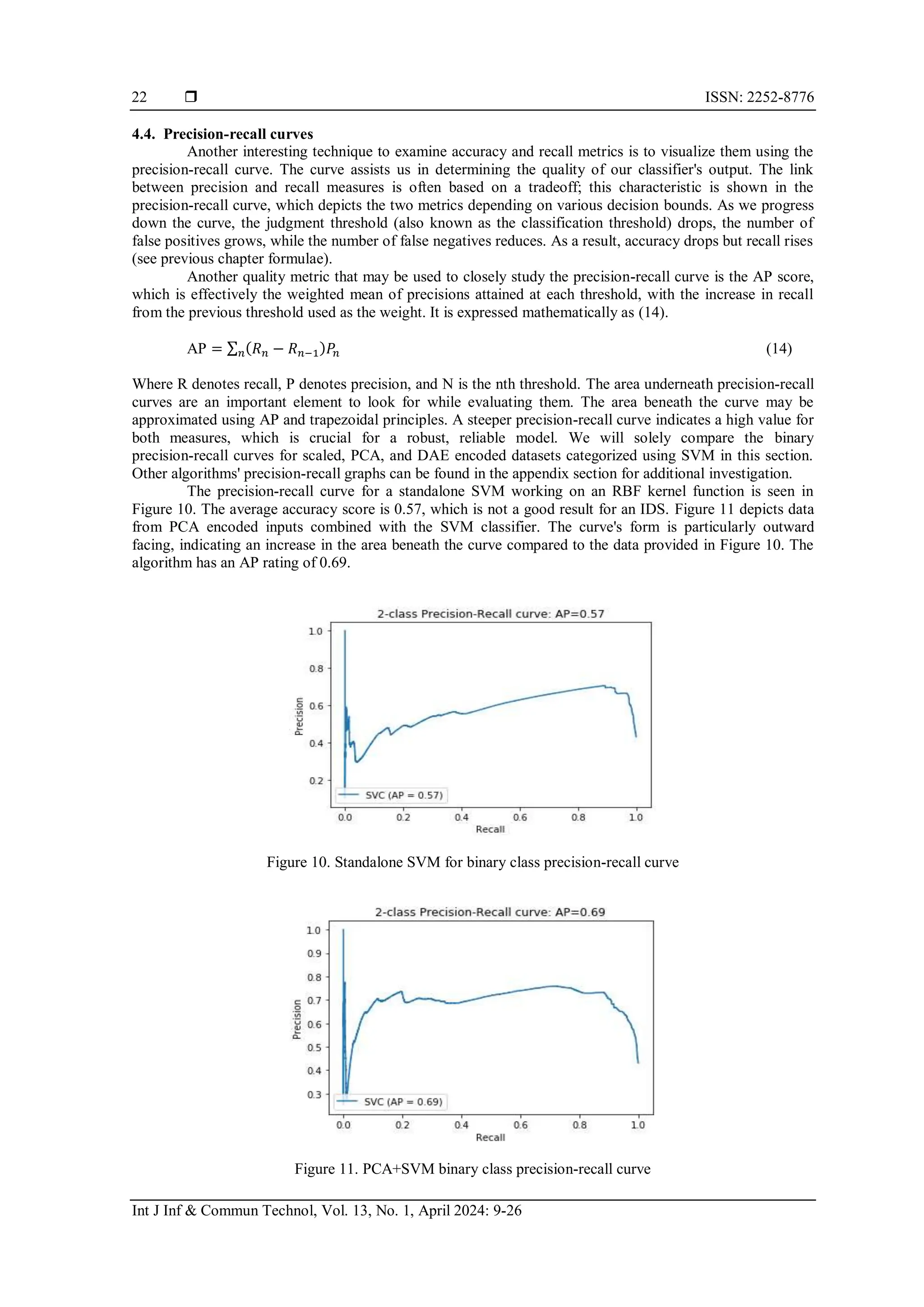
3.8. Precision-recall curve
The precision and recall metrics are very important measures when dealing with imbalanced classes.
Precision calculates the proportion of positive identifications that were correct. It could be mathematically
defined as (11).
𝑃𝑟𝑒𝑐𝑖𝑠𝑖𝑜𝑛 =
𝑇𝑃
𝑇𝑃+𝐹𝑃
(11)
Recall is defined as the proportion of actual positives correctly identified. It can be written as (12).
𝑅𝑒𝑐𝑎𝑙𝑙 =
𝑇𝑃
𝑇𝑃+𝐹𝑁
(12)
As the decision threshold is increased, there is usually a trade-off between precision and recall.
When the categorization threshold is raised, the recall either decreases or remains constant. In contrast,
increasing the classification threshold improves accuracy [36]. The precision-recall curve visually depicts the
inverse connection.
3.9. F-measure
The F-measure is a statistic with a single value that is based on precision and recall. The F-measure
has a value between 0 and 1. The F-measure allows for the simultaneous consideration of accuracy and recall
through a single measure, as opposed to seeing them as trade-offs. The F-measure is mathematically defined
as (13).
𝐹𝑀 =
(1+𝛽1)∗𝑅𝑒𝑐𝑎𝑙𝑙∗𝑃𝑟𝑒𝑐𝑖𝑠𝑖𝑜𝑛
𝑅𝑒𝑐𝑎𝑙𝑙+𝑃𝑟𝑒𝑐𝑖𝑠𝑖𝑜𝑛
(13)

 ISSN: 2252-8776
18
3.10. Test and train timings
Network-level assaults are time-sensitive. Therefore, the test and train timings are critical for this
investigation. As a result, having a model that can train significantly quicker than other methods would be
extremely beneficial to our research.
4. RESULTS
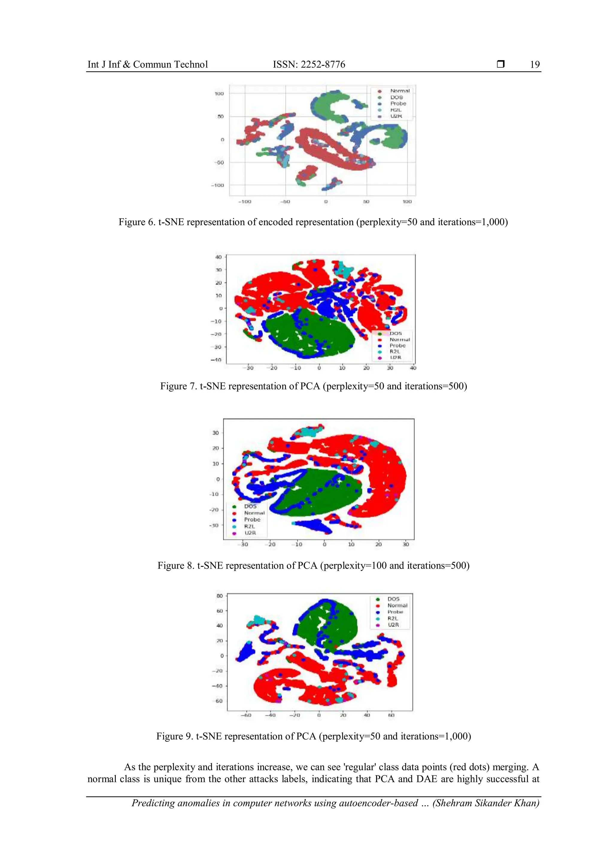
4.1. Visualizing data using t-distributed stochastic neighbor embedding
We use t-distributed stochastic neighbor embedding (t-SNE), a method for displaying high
dimensional data, to visualize our dataset. t-SNE makes use of kullback-leibler (KL) divergence, a measure
of the difference between two probability distributions [37]. KL divergence may be seen of as a
dimensionality reduction approach since it translates observations into joint probabilities, which reduces the
amount of information processed overall. When dealing with larger dimensional data (usually more than 50
dimensions), it is advised to use a previous dimensionality reduction approach to produce a manageable
subspace that t-SNE can handle well because it requires a significant amount of computer resources.
Furthermore, applying t-SNE on smaller dimensions handles noise without distorting interpoint distances. In
our case, we'd use PCA (linear dimensionality reduction) and DAE (non-linear dimensionality reduction) to
evaluate how t-SNE visualizes the decreased dimensions from both methods. Using DAE, we were able to
reduce the initial feature space of 122 inputs to a subspace of 10 dimensions. For our dataset, we will use
t-SNE to display a 2D manifold with varying perplexity levels. Perplexity can be regarded as a smooth
measure of the number of effective neighbors. Perplexity levels typically range from 5 to 50. When working
with bigger datasets, however, it is acceptable to use a greater perplexity number. The t-SNE representation
of AE encoded dimensions can be shown in Figures 4-6, whereas PCA dimensions with altered perplexity
and iterations can be seen in Figures 7-9. We can see that at increasing perplexity and iterations, both AE and
PCA are able to cluster various attack groups more effectively than in lower perplexity and iterations. The
data points in all figures are color-coded according to the NSL-KDD dataset's five assault classifications. The
graph above's vertical and horizontal axes are formed using the KL divergence technique, which is used to
embed a high dimensional data space into a smaller subspace.
Figure 4. t-SNE representation of encoded representation (perplexity=50 and iterations=500)
Figure 5. t-SNE representation of encoded representation (perplexity=100 and iterations=500)

19
Figure 6. t-SNE representation of encoded representation (perplexity=50 and iterations=1,000)
Figure 7. t-SNE representation of PCA (perplexity=50 and iterations=500)
Figure 8. t-SNE representation of PCA (perplexity=100 and iterations=500)
Figure 9. t-SNE representation of PCA (perplexity=50 and iterations=1,000)
As the perplexity and iterations increase, we can see 'regular' class data points (red dots) merging. A
normal class is unique from the other attacks labels, indicating that PCA and DAE are highly successful at

 ISSN: 2252-8776
20
distinguishing between 'normal' and 'attack'. However, when we focus on the other four attack classes, we
observe a different picture; with the exception of the 'DOS' attack class, the other three attack classes are
jumbled together and do not form a discernible cluster. The t-SNE representation of PCA and the DAE hint
that categorizing the other three assault methods may be difficult.
4.2. Grid search
We used the GridSearchCV provided via scikit-learn, an open-source ML package accessible on
Python, to optimize the parameters for our classifier. The GridSearchCV aims to execute an exhaustive
search across supplied parameter values for our SVM classifier based on important score. Table 2 illustrates
the Grid Search with 'Balanced Accuracy' Scoring for our purposes.
The γ and c parameters are important to consider while dealing with SVM using RBF Kernel
function. The c variable may be thought of as a regularization term that keeps sparse variables in control. The
ideal parameter selection is determined by the degree of noise and balance in the dataset. We used the kernel
methods provided in the scikit-learn python package because our dataset was non-linear. We have four kernel
functions to pick from: linear, polynomial, RBF, and sigmoid. As indicated in Table 3, we used 'RBF' for our
investigation since our grid search projected RBF to be the optimum kernel function for optimizing f1-micro.
Table 2. Grid search with 'balanced accuracy' scoring
Balanced accuracy Std C Kernel
0.458 (+/-0.035) 1 Linear
0.823 (+/-0.094) 1 RBF
0.755 (+/-0.081) 1 Poly
0.611 (+/-0.056) 10 Linear
0.841 (+/-0.154) 10 RBF
0.851 (+/-0.100) 10 Poly
0.66 (+/-0.079) 100 Linear
0.849 (+/-0.126) 100 RBF
0.875 (+/-0.106) 100 Poly
0.688 (+/-0.109) 1,000 Linear
0.828 (+/-0.091) 1,000 RBF
0.845 (+/-0.135) 1,000 Poly
Table 3. Grid search with 'f1-micro' scoring
F1-micro score Std C Kernel
0.704 (+/-0.258) 1 Linear
0.815 (+/-0.011) 1 RBF
0.781 (+/-0.019) 1 Poly
0.497 (+/-0.017) 10 Linear
0.883 (+/-0.010) 10 RBF
0.851 (+/-0.013) 10 Poly
0.567 (+/-0.023) 100 Linear
0.928 (+/-0.011) 100 RBF
0.903 (+/-0.014) 100 Poly
0.665 (+/-0.028) 1,000 Linear
0.949 (+/-0.013) 1,000 RBF
0.937 (+/-0.012) 1,000 Poly
4.3. Classification metrics: accuracy, precision-recall, and f-score
In this section, we will thoroughly study three primary models to understand their efficacy at
predicting anomalies as well as the quality of their forecast by looking at subtler yet significant variables like
as accuracy, recall, and f-score. Simply looking at accuracy is insufficient to assess our model's efficacy,
especially given the NSL-KDD dataset's uneven label distribution. We must pay special attention to
examining recall values for the models in issue since false negatives (type 1 mistake) might generate
incursions that could lead to a breach in the information system of another individual or business. To avoid
such scenario, the recall metric is extremely important to us as cybersecurity specialists.
It is also necessary to examine the accuracy, recall, and f1-score values of various attack types, since
this will provide us with a clearer view of the model's performance. For example, failing to have a high recall
in a U2R attack type might result in a hacker gaining root access to the system. Thus, if we want to construct
a robust anomaly-based IDS, we need to measure our models' performance against specific attack types as
well as focus on the overall model. The first model we'll look at is a solo SVM model with input data scaled
using L2 normalization. The model's predictions are created against an unknown validation set supplied by
the NSL-KDD. The total prediction accuracy in the binary label scenario illustrated in Table 4 is 77%, while
the model provides a weighted average f1-score of 76%. In Table 5, we use the same model on a multi-class
scenario where attack label is further divided into four classes. The overall accuracy as well as weighted f1,
recall, and precision drop quite significantly when performing multi-label predictions.
The second model combines dimensionality reduction with PCA and SVM that has been similarly
tweaked. Based on the binary data in Table 6, we see a 74% reduction in accuracy and recall. Only for
multiclass labels, we found a drop in weighted averages for recall, f1-score, precision, and overall accuracy
when compared to the multiclass solo SVM model, as shown in Table 7.
According to Table 8, our suggested approach significantly improves accuracy and average recall
rates when dealing with binary labels. As a result, while dealing with many classes, our suggested model
outperforms the previous two models in terms of weighted averages of precision, recall, and f1-score, as well
as accuracy. However, when we focus on U2R, we find that the recall rates are significantly greater in the
solo SVM scenario than in our model, as shown in Table 9.

21
Table 4. Binary label classification report for standalone SVM
Label Precision (%) Recall (%) F1-score (%) Support
Normal 65 97 78 9,711
Attack 97 61 75 12,833
Other measures
Accuracy 77 22,544
Macro average 81 79 77 22,544
Weighted average 83 77 76 22,544
Table 5. Multi-label classification report for standalone SVM
Normal 70 84 77 9,711
DOS 90 70 79 7,460
Probe 59 62 60 2,421
R2L 42 23 30 2,885
U2R 4 60 8 67
Other measures
Accuracy 69 22,544
Table 6. Binary label classification report for PCA+SVM classifier
Normal 63 96 76 9,711
Attack 95 56 71 12,833
Other measures
Accuracy 74 22,544
Table 7. Multi-label classification report for PCA+SVM classifier
Normal 61 55 58 9,711
DOS 88 68 77 7,460
Probe 48 63 54 2,421
R2L 19 10 13 2,885
U2R 1 52 2 67
Other measures
Accuracy 55 22,544
Table 8. Binary label classification report for AE encoded+SVM classifier (L2 regularization)
Normal 67 97 80 9,711
Attack 96 65 77 12,833
Other measures
Accuracy 78 22,544
Weightedaverage 84 78 78 22,544
Table 9. Multi-label classification report for AE encoded+SVM classifier
Label Precision Recall F1-score Support
Normal 71% 89% 79% 9711
DOS 90% 74% 81% 7460
Probe 70% 62% 65% 2421
R2L 50% 23% 32% 2885
U2R 5% 48% 9% 67
Other measures
Accuracy 73% 22544
Macro average 57% 59% 53% 22544
Weighted average 74% 73% 72% 22544

 ISSN: 2252-8776
22
4.4. Precision-recall curves
Another interesting technique to examine accuracy and recall metrics is to visualize them using the
precision-recall curve. The curve assists us in determining the quality of our classifier's output. The link
between precision and recall measures is often based on a tradeoff; this characteristic is shown in the
precision-recall curve, which depicts the two metrics depending on various decision bounds. As we progress
down the curve, the judgment threshold (also known as the classification threshold) drops, the number of
false positives grows, while the number of false negatives reduces. As a result, accuracy drops but recall rises
(see previous chapter formulae).
Another quality metric that may be used to closely study the precision-recall curve is the AP score,
which is effectively the weighted mean of precisions attained at each threshold, with the increase in recall
from the previous threshold used as the weight. It is expressed mathematically as (14).
AP = ∑ (𝑅𝑛 − 𝑅𝑛−1)𝑃
𝑛
𝑛 (14)
Where R denotes recall, P denotes precision, and N is the nth threshold. The area underneath precision-recall
curves are an important element to look for while evaluating them. The area beneath the curve may be
approximated using AP and trapezoidal principles. A steeper precision-recall curve indicates a high value for
both measures, which is crucial for a robust, reliable model. We will solely compare the binary
precision-recall curves for scaled, PCA, and DAE encoded datasets categorized using SVM in this section.
Other algorithms' precision-recall graphs can be found in the appendix section for additional investigation.
The precision-recall curve for a standalone SVM working on an RBF kernel function is seen in
Figure 10. The average accuracy score is 0.57, which is not a good result for an IDS. Figure 11 depicts data
from PCA encoded inputs combined with the SVM classifier. The curve's form is particularly outward
facing, indicating an increase in the area beneath the curve compared to the data provided in Figure 10. The
algorithm has an AP rating of 0.69.
Figure 10. Standalone SVM for binary class precision-recall curve
Figure 11. PCA+SVM binary class precision-recall curve

23
This graph in Figure 12 clearly demonstrates the precision-recall trade-off described at the
beginning of this section. We can see that when the choice boundary shrinks, the recall grows. The region
beneath the curve is clearly larger than in the preceding two plots of SVM and PCA-SVM, respectively. Our
suggested model has an AP score of 0.90, which is rather high. We employ the models in multiclass, but with
an additional weight balancing modification. Because the precision-recall curve is mostly utilized for binary
labels, we shall binarize distinct curves for the five classes. Because our dataset has a class imbalance, we
elected to micro-average rather than macro-average all five classes, which may result in a different
interpretation.
Figure 13 depicts precision-recall curves for normalized inputs based on a solo SVM classifier. The
micro-average of precision-recall curves for all five classes, computed by aggregating the contributions of the
five classes, is an essential statistic in the preceding graph. According to the curves in Figure 14, PCA
encoded inputs result in a significant rise in the micro-average of precision-recall, specifically from 0.59 to
0.63. It should be noted that our graphics show iso curves at various f1 values. Iso-curves are convex-shaped
curves that, for a given f1-score, follow a combination of precision and recall values. The iso-curves provide
a consistent reference point for better understanding of the precision-recall curve. Figure 15 depicts data from
DAE inputs categorized using SVM. The data shows a significantly higher micro-average than the prior two
models. The area under the micro-AP recall curve is 0.72, which is 10 basis points more than the prior model.
Figure 12. AE+SVM precision-recall curve (polynomial kernel)
Figure 13. Standalone SVM for multiclass precision-recall curves

 ISSN: 2252-8776
24
Figure 14. PCA+SVM multiclass precision-recall
curves
Figure 15. AE+SVM multiclass precision-recall
curves
4.5. Performance metrics: train and test time
One of the most essential characteristics of a successful model is the amount of time and processing
resources required to make its forecasts. We utilized Python's time module to calculate how long it takes our
models to train and test on the NSL-KDD dataset. The training and testing times for the algorithms employed
in this work are shown in Table 10 in seconds. Based on our findings, we can infer that L1 regularized DAE
combined with SVM saves the greatest time when dealing with binary classes. In the multi-class situation, we
discover that DAE-SVM without any regularization term takes the least amount of time to train and test the
NSL-KDD dataset, providing a clear response to our initial research question about the usefulness of an
autoencoder-based dimensionality reduction technique. In both multi and binary class contexts, a standalone
SVM appears to take the most time.
Table 10. Train and test time based on seconds
Algorithm Training_Time (sec) Testing_Time (sec) Total_Time (sec) Class
SVM 392.70 39.68 432.38 Binary
DAE-SVM 59.13+86.60 2.28 148.01 Binary
DAE-SVM L1 52.55+90.49 2.80 145.84* Binary
DAE-SVM L2 62.22+89.64 2.69 154.53 Binary
SVM 1545.64 133.23 1,678.87 Multi-class
PCA-SVM 270.16 29.83 299.99 Multi-class
DAE-SVM 48.09+89.75 7.78 145.62* Multi-class
DAE-SVM L1 49.20+121.04 10.72 180.96 Multi-class
DAE-SVM L2 48.60+114.15 9.51 172.26* Multi-class
*Algorithm that takes the least time to train and test on the NSL-KDD dataset
5. CONCLUSION
The findings of this study covered all of the themes raised in the research question section. To
summarize our findings, we discovered that a DAE+SVM-based neural network method was successful
based on several classification and performance criteria. When t-SNE was used to embed higher dimension
inputs on a two-dimensional plane and was compared to its linear PCA equivalent, autoencoders were
substantially more effective at capturing valuable features of inputs. In particular, in terms of training and
testing time, autoencoder encoded inputs showed to be substantially more time-efficient during the model's
training and testing phases. Furthermore, our proposed neural system outperforms solo SVM and PCA
encoded SVM in multi-class classification metrics such as weighted average of recall, f-score, and Accuracy.

25
We were able to acquire a more precise perspective of our suggested neural scheme's performance by
focusing on type 1 (false positives) and type II (false negatives) mistakes by focusing on measures such as
accuracy and recall. Because we are dealing with anomaly detection, we should place greater emphasis on
type II error because enabling an anomaly to permeate our IDS has the ability to wreak havoc on our system's
resources. After thoroughly studying the classification metrics, we can confidently conclude that
autoencoders are a feasible dimensionality reduction approach when compared to PCA for anomaly detection
on the NSL-KDD Dataset.
REFERENCES
[1] N. Harale and B. B. Meshram, “Network based intrusion detection and prevention systems: attack classification, methodologies
and tools,” Research Inventy: International Journal of Engineering And Science, vol. 6, no. 5, pp. 1–12, 2016.
[2] A. M. Dissanayaka, S. Mengel, R. R. Shetty, L. Gittner, S. Kothari, and R. Vadapalli, “A review of MongoDB and singularity
container security in regards to HIPAA regulations,” UCC 2017 Companion-Companion Proceedings of the 10th International
Conference on Utility and Cloud Computing, pp. 91–97, 2017, doi: 10.1145/3147234.3148133.
[3] “Secure NoSQL based medical data processing and retrieval,” in UCC 2017 Companion - Companion Proceedings of the 10th
International Conference on Utility and Cloud Computing, 2017, pp. 99–105. doi: 10.1145/3147234.3148132.
[4] S. Thapa and M. Bissanayaka, Akalanka, “The role of intrusion detection/prevention systems in modern computer networks: a
review,” Midwest Instruction and Computing Symposium (MICS), vol. 53, pp. 1–14, 2020.
[5] A. B. Mailewa, S. Mengel, L. Gittner, H. Khan, and A. M. Dissanayaka, “Dynamic and portable vulnerability assessment testbed
with linux containers to ensure the security of MongoDB in singularity LXCs dynamic and portable vulnerability assessment
testbed with linux containers to ensure the security of MongoDB in singularity ,” pp. 1–5, 2018.
[6] M. K. Asif, T. A. Khan, T. A. Taj, U. Naeem, and S. Yakoob, “Network intrusion detection and its strategic importance,” 2013
IEEE Business Engineering and Industrial Applications Colloquium (BEIAC), pp. 140–144, 2013, doi:
10.1109/BEIAC.2013.6560100.
[7] N. Shone, T. N. Ngoc, V. D. Phai, and Q. Shi, “A deep learning approach to network intrusion detection,” IEEE Transactions on
Emerging Topics in Computational Intelligence, vol. 2, no. 1, pp. 41–50, 2018, doi: 10.1109/TETCI.2017.2772792.
[8] E. Simkhada, E. Shrestha, S. Pandit, U. Sherchand, and A. M. Dissanayaka, “Security threats/attacks via botnets and botnet
detection and prevention techniques in computer networks: a review,” The Midwest Instruction and Computing
Symposium.(MICS), North Dakota State University, Fargo, ND, pp. 1–15, 2019.
[9] A. M. Dissanayaka, S. Mengel, L. Gittner, and H. Khan, “Vulnerability prioritization, root cause analysis, and mitigation of
secure data analytic framework implemented with mongodb on singularity linux containers,” ACM International Conference
Proceeding Series, pp. 58–66, 2020, doi: 10.1145/3388142.3388168.
[10] J. Gu, L. Wang, H. Wang, and S. Wang, “A novel approach to intrusion detection using SVM ensemble with feature
augmentation,” Computers and Security, vol. 86, pp. 53–62, 2019, doi: 10.1016/j.cose.2019.05.022.
[11] A. M. Dissanayaka, S. Mengel, L. Gittner, and H. Khan, “Security assurance of MongoDB in singularity LXCs: an elastic and
convenient testbed using Linux containers to explore vulnerabilities,” Cluster Computing, vol. 23, no. 3, pp. 1955–1971, 2020,
doi: 10.1007/s10586-020-03154-7.
[12] S. Naseer et al., “Enhanced network anomaly detection based on deep neural networks,” IEEE Access, vol. 6, pp. 48231–48246,
2018, doi: 10.1109/ACCESS.2018.2863036.
[13] S. Mukkamala, G. Janoski, and A. Sung, “Intrusion detection using neural networks and support vector machines,” Proceedings
of the International Joint Conference on Neural Networks, vol. 2, pp. 1702–1707, 2002, doi: 10.1109/ijcnn.2002.1007774.
[14] Y. Liao and V. R. Vemuri, “Use of k-nearest neighbor classifier for intrusion detection,” Computers & Security, vol. 21, no. 5, pp.
439–448, Oct. 2002, doi: 10.1016/S0167-4048(02)00514-X.
[15] Z. Chiba, N. Abghour, K. Moussaid, A. El omri, and M. Rida, “Intelligent approach to build a Deep Neural Network based IDS
for cloud environment using combination of machine learning algorithms,” Computers & Security, vol. 86, pp. 291–317, Sep.
2019, doi: 10.1016/j.cose.2019.06.013.
[16] C. Xenakis, C. Panos, and I. Stavrakakis, “A comparative evaluation of intrusion detection architectures for mobile ad hoc
networks,” Computers & Security, vol. 30, no. 1, pp. 63–80, Jan. 2011, doi: 10.1016/j.cose.2010.10.008.
[17] M. Tavallaee, E. Bagheri, W. Lu, and A. A. Ghorbani, “A detailed analysis of the KDD CUP 99 data set,” IEEE Symposium on
Computational Intelligence for Security and Defense Applications, CISDA 2009, pp. 1–6, 2009, doi:
10.1109/CISDA.2009.5356528.
[18] P. Burnap, R. French, F. Turner, and K. Jones, “Malware classification using self organising feature maps and machine activity
data,” Computers & Security, vol. 73, pp. 399–410, Mar. 2018, doi: 10.1016/j.cose.2017.11.016.
[19] S. Ni, Q. Qian, and R. Zhang, “Malware identification using visualization images and deep learning,” Computers & Security, vol.
77, pp. 871–885, Aug. 2018, doi: 10.1016/j.cose.2018.04.005.
[20] S.-H. Wang, P. Phillips, Y. Sui, B. Liu, M. Yang, and H. Cheng, “Classification of alzheimer’s disease based on eight-layer
convolutional neural network with leaky rectified linear unit and max pooling,” Journal of Medical Systems, vol. 42, no. 5, pp. 1–
11, May 2018, doi: 10.1007/s10916-018-0932-7.
[21] P. Ramachandran, B. Zoph, and Q. V. Le, “Searching for activation functions,” in 6th International Conference on Learning
Representations, ICLR 2018 - Workshop Track Proceedings, Oct. 2017. doi: 1710.05941 Focus to learn more.
[22] T. Unterthiner, G. Klambauer, S. Hochreiter, and A. Mayr, “Self-normalizing neural networks,” in Advances In Neural
Information Processing Systems, 2017.
[23] Y. Wang, H. Yao, and S. Zhao, “Auto-encoder based dimensionality reduction,” Neurocomputing, vol. 184, pp. 232–242, Apr.
2016, doi: 10.1016/j.neucom.2015.08.104.
[24] L. Van Der Maaten, E. Postma, J. V. den H.-J. M. L. Res, and U. 2009, “Dimensionality reduction: a comparative,” Journal of
Machine Learning Research, vol. 10, pp. 1–41, 2009.
[25] P. Vincent, H. Larochelle, I. Lajoie, Y. Bengio, and P. A. Manzagol, “Stacked denoising autoencoders: learning useful representations
in a deep network with a local denoising criterion,” Journal of Machine Learning Research, vol. 11, pp. 3371–3408, 2010.
[26] J. Masci, U. Meier, D. Cireşan, and J. Schmidhuber, “Stacked convolutional auto-encoders for hierarchical feature extraction,” in
Lecture Notes in Computer Science (including subseries Lecture Notes in Artificial Intelligence and Lecture Notes in
Bioinformatics), 2011, pp. 52–59. doi: 10.1007/978-3-642-21735-7_7.

 ISSN: 2252-8776
26
[27] S. Rifai, P. Vincent, X. Muller, X. Glorot, and Y. Bengio, “Contractive auto-encoders: Explicit invariance during feature
extraction,” in Proceedings of the 28th International Conference on Machine Learning, 2011, pp. 833–840.
[28] Q. Xu, C. Zhang, L. Zhang, and Y. Song, “The learning effect of different hidden layers stacked autoencoder,” in Proceedings -
2016 8th International Conference on Intelligent Human-Machine Systems and Cybernetics, (IHMSC ), 2016, pp. 148–151. doi:
10.1109/IHMSC.2016.280.
[29] O. Demir-Kavuk, M. Kamada, T. Akutsu, and E.-W. Knapp, “Prediction using step-wise L1, L2 regularization and feature
selection for small data sets with large number of features,” BMC Bioinformatics, vol. 12, no. 1, pp. 1–10, Dec. 2011, doi:
10.1186/1471-2105-12-412.
[30] A. Shenfield, D. Day, and A. Ayesh, “Intelligent intrusion detection systems using artificial neural networks,” ICT Express, vol.
4, no. 2, pp. 95–99, Jun. 2018, doi: 10.1016/j.icte.2018.04.003.
[31] M. Al-Qatf, Y. Lasheng, M. Al-Habib, and K. Al-Sabahi, “Deep learning approach combining sparse autoencoder with SVM for
network intrusion detection,” IEEE Access, vol. 6, pp. 52843–52856, 2018, doi: 10.1109/ACCESS.2018.2869577.
[32] M. Yousefi-Azar, V. Varadharajan, L. Hamey, and U. Tupakula, “Autoencoder-based feature learning for cyber security
applications,” in Proceedings of the International Joint Conference on Neural Networks, 2017, pp. 3854–3861. doi:
10.1109/IJCNN.2017.7966342.
[33] B. Lee, S. Amaresh, C. Green, and D. Engels, “Comparative study of deep learning models for network intrusion detection,” SMU
Data Science Review, vol. 1, 2018.
[34] J. J. Davis and A. J. Clark, “Data preprocessing for anomaly based network intrusion detection: a review,” Computers & Security,
vol. 30, no. 6–7, pp. 353–375, Sep. 2011, doi: 10.1016/j.cose.2011.05.008.
[35] N. Seliya, T. M. Khoshgoftaar, and J. Van Hulse, “A study on the relationships of classifier performance metrics,” in
Proceedings-International Conference on Tools with Artificial Intelligence, ICTAI, 2009, pp. 59–66. doi: 10.1109/ICTAI.2009.25.
[36] R. S. M. Carrasco and M.-A. Sicilia, “Unsupervised intrusion detection through skip-gram models of network behavior,”
Computers & Security, vol. 78, pp. 187–197, Sep. 2018, doi: 10.1016/j.cose.2018.07.003.
[37] L. van der Maaten and G. Hinton, “Visualizing data using t-SNE,” Journal of machine learning research, vol. 9, pp. 2579–2605,
2008.
BIOGRAPHIES OF AUTHORS
Shehram Sikander Khan received his M.Sc. in Information Assurance from
St. Cloud State University in spring 2020. He is an experienced Business Intelligence
Analyst with deep expertise in data warehousing, process validation and business needs
analysis. He has proven ability to understand customer requirements and translate into
actionable project plans. Also, he dedicated and hard-working with a passion for Data
Analysis. He has a thorough knowledge of project management, database design, strategic
planning, data visualization, and machine learning. He is currently working as a Business
Intelligence Analyst at Global Overview, Marketing and Advertising, Minnetonka,
Minnesota, USA. He can be contacted at email: shehram.khan@go.stcloudstate.edu.
Akalanka Bandara Mailewa (Dissanayaka Mohottalalage) earned his Ph.D.
in Computer Science from Texas Tech University, Lubbock, Texas, USA in Spring 2020 and
his Ph.D. dissertation research focuses on implementation of secure big data analytic
framework with MongoDB and Linux Containers in high performance clusters (HPC) in
regards to HIPAA regulations. He received his M.Sc. in Computer Science from Saint Cloud
State University, Saint Cloud, Minnesota, USA and earned his B·Sc. Engineering (Hons) in
Computer Engineering from University of Peradeniya, Kandy, Sri Lanka. In industry, he
worked in multiple fulltime roles such as; Network Engineer, Systems Administrator,
Software Developer, and Software Test Automation Engineer. He is certified with several
Microsoft certifications such as MCP, MCTS, MCSA, MCITP, MCSE, and MCSE-security
while he has followed RHCT and CCNA courses. In addition, he is a Palo-Alto Networks
Authorized Cybersecurity Academy Instructor with CIC and CPC certifications. His
research interest includes Big-data security, IoT security, cryptography, ethical hacking,
penetration testing, and software test automation. In various research areas, he has published
several scientific journal articles and conference proceedings by presenting in several well-
known conferences. Also, he is serving as an editorial board member and a reviewer of
several journals and conferences. In addition, he has received several fellowships, awards,
and travel grants from various institutes and organizations. Overall, about 15 years of
teaching experiences in higher education, he is currently working as a tenure-track assistant
professor in the department of computer science and information technology at Saint Cloud
State University, Saint Cloud, Minnesota, USA. He can be contacted at email:
amailewa@stcloudstate.edu.

Predicting anomalies in computer networks using autoencoder based representation learning

More Related Content

Similar to Predicting anomalies in computer networks using autoencoder based representation learning

More from IJICTJOURNAL

Recently uploaded

Predicting anomalies in computer networks using autoencoder based representation learning