Practical Optimization: Algorithms and Engineering Applications 2nd Edition Andreas Antoniou
Practical Optimization: Algorithms and Engineering Applications 2nd Edition Andreas Antoniou
Practical Optimization: Algorithms and Engineering Applications 2nd Edition Andreas Antoniou


![1.1 Introduction 3
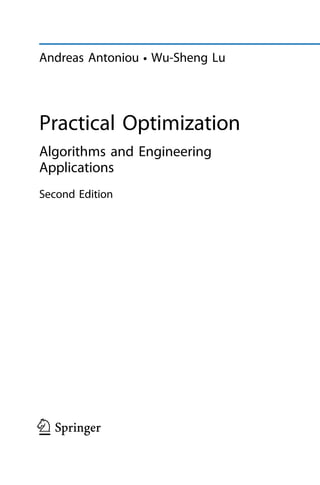
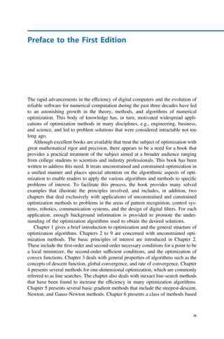
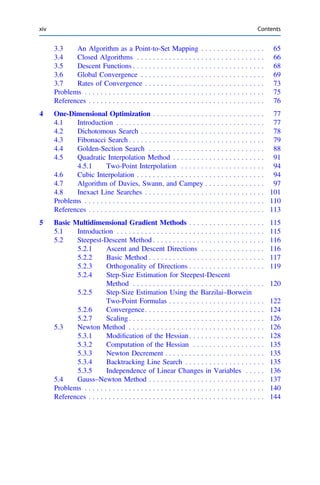
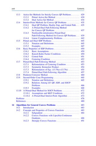
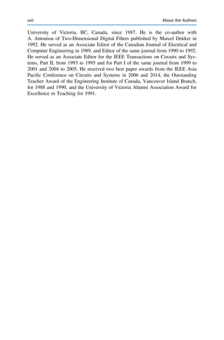
Fig.1.1 Contour plot of
f (x1, x2)
A
10
f (x , x ) = 0
1 2
f (x , x ) = 50
1 2
1
x
2
x
20
30
40
50
each other, and must be adjusted simultaneously to yield the optimum performance
criterion.
The most important general approach to optimization is based on numerical meth-
ods. In this approach, iterative numerical procedures are used to generate a series
of progressively improved solutions to the optimization problem, starting with an
initial estimate for the solution. The process is terminated when some convergence
criterion is satisfied. For example, when changes in the independent variables or the
performance criterion from iteration to iteration become insignificant.
Numerical methods can be used to solve highly complex optimization problems
of the type that cannot be solved analytically. Furthermore, they can be readily
programmed on the digital computer. Consequently, they have all but replaced most
other approaches to optimization.
The discipline encompassing the theory and practice of numerical optimization
methods has come to be known as mathematical programming [1–5]. During the past
40 years, several branches of mathematical programming have evolved, as follows:
1. Linear programming
2. Integer programming
3. Quadratic programming
4. Nonlinear programming
5. Dynamic programming
Each one of these branches of mathematical programming is concerned with a spe-
cific class of optimization problems. The differences among them will be examined
in Sect.1.6.](https://image.slidesharecdn.com/20986-250315065426-4aaea085/85/Practical-Optimization-Algorithms-and-Engineering-Applications-2nd-Edition-Andreas-Antoniou-30-320.jpg)
![4 1 The Optimization Problem
1.2 The Basic Optimization Problem
Before optimization is attempted, the problem at hand must be properly formulated.
A performance criterion F must be derived in terms of n parameters x1, x2, . . . , xn
as
F = f (x1, x2, . . . , xn)
F is a scalar quantity which can assume numerous forms. It can be the cost of a
product in a manufacturing environment or the difference between the desired per-
formance and the actual performance in a system. Variables x1, x2, . . . , xn are the
parameters that influence the product cost in the first case or the actual performance in
the second case. They can be independent variables, like time, or control parameters
that can be adjusted.
The most basic optimization problem is to adjust variables x1, x2, . . . , xn in
such a way as to minimize quantity F. This problem can be stated mathematically
as
minimize F = f (x1, x2, . . . , xn) (1.1)
Quantity F is usually referred to as the objective or cost function.
The objective function may depend on a large number of variables, sometimes as
many as 100 or more. To simplify the notation, matrix notation is usually employed.
If x is a column vector with elements x1, x2, . . . , xn, the transpose of x, namely,
xT , can be expressed as the row vector
xT
= [x1 x2 · · · xn]
In this notation, the basic optimization problem of Eq. (1.1) can be expressed as
minimize F = f (x) for x ∈ En
where En represents the n-dimensional Euclidean space.
On many occasions, the optimization problem consists of finding the maximum
of the objective function. Since
max[ f (x)] = −min[− f (x)]
the maximum of F can be readily obtained by finding the minimum of the negative of
F and then changing the sign of the minimum. Consequently, in this and subsequent
chapters we focus our attention on minimization without loss of generality.
In many applications, a number of distinct functions of x need to be optimized
simultaneously. For example, if the system of nonlinear simultaneous equations
fi (x) = 0 for i = 1, 2, . . . , m
needs to be solved, a vector x is sought which will reduce all fi (x) to zero simulta-
neously. In such a problem, the functions to be optimized can be used to construct a
vector
F(x) = [ f1(x) f2(x) · · · fm(x)]T
The problem can be solved by finding a point x = x∗ such that F(x∗) = 0. Very
frequently, a point x∗ that reduces all the fi (x) to zero simultaneously may not](https://image.slidesharecdn.com/20986-250315065426-4aaea085/85/Practical-Optimization-Algorithms-and-Engineering-Applications-2nd-Edition-Andreas-Antoniou-31-320.jpg)
![1.2 The Basic Optimization Problem 5
exist but an approximate solution, i.e., F(x∗) ≈ 0, may be available which could be
entirely satisfactory in practice.
A similar problem arises in scientific or engineering applications when the func-
tion of x that needs to be optimized is also a function of a continuous independent
parameter (e.g., time, position, speed, frequency) that can assume an infinite set
of values in a specified range. The optimization might entail adjusting variables
x1, x2, . . . , xn so as to optimize the function of interest over a given range of the
independent parameter. In such an application, the function of interest can be sampled
with respect to the independent parameter, and a vector of the form
F(x) = [ f (x, t1) f (x, t2) · · · f (x, tm)]T
can be constructed, where t is the independent parameter. Now if we let
fi (x) ≡ f (x, ti )
we can write
F(x) = [ f1(x) f2(x) · · · fm(x)]T
A solution of such a problem can be obtained by optimizing functions fi (x) for
i = 1, 2, . . . , m simultaneously. Such a solution would, of course, be approximate
because any variations in f (x, t) between sample points are ignored. Nevertheless,
reasonable solutions can be obtained in practice by using a sufficiently large number
of sample points. This approach is illustrated by the following example.
Example 1.1 The step response y(x, t) of an nth-order control system is required
to satisfy the specification
y0(x, t) =
⎧
⎪
⎪
⎨
⎪
⎪
⎩
t for 0 ≤ t < 2
2 for 2 ≤ t < 3
−t + 5 for 3 ≤ t < 4
1 for 4 ≤ t
as closely as possible. Construct a vector F(x) that can be used to obtain a function
f (x, t) such that
y(x, t) ≈ y0(x, t) for 0 ≤ t ≤ 5
Solution The difference between the actual and specified step responses, which
constitutes the approximation error, can be expressed as
f (x, t) = y(x, t) − y0(x, t)
and if f (x, t) is sampled at t = 0, 1, . . . , 5, we obtain
F(x) = [ f1(x) f2(x) · · · f6(x)]T](https://image.slidesharecdn.com/20986-250315065426-4aaea085/85/Practical-Optimization-Algorithms-and-Engineering-Applications-2nd-Edition-Andreas-Antoniou-32-320.jpg)
![1.2 The Basic Optimization Problem 7
Several special cases of the L p norm are of particular interest. If p = 1
F ≡ L1 =
m
i=1
| fi (x)|
and, therefore, in a minimization problem like that in Example1.1, the sum of the
magnitudes of the individual element functions is minimized. This is called an L1
problem.
If p = 2, the Euclidean norm
F ≡ L2 =
m
i=1
| fi (x)|2
1/2
is minimized, and if the square root is omitted, the sum of the squares is minimized.
Such a problem is commonly referred to as a least-squares problem.
In the case where p = ∞, if we assume that there is a unique maximum of | fi (x)|
designated F̂ such that
F̂ = max
1≤i≤m
| fi (x)|
then we can write
F ≡ L∞ = lim
p→∞
m
i=1
| fi (x)|p
1/p
= F̂ lim
p→∞
m
i=1
| fi (x)|
F̂
p
1/p
Since all the terms in the summation except one are less than unity, they tend to zero
when raised to a large positive power. Therefore, we obtain
F = F̂ = max
1≤i≤m
| fi (x)|
Evidently, if the L∞ norm is used in Example1.1, the maximum approximation error
is minimized and the problem is said to be a minimax problem.
Often the individual element functions of F(x) are modified by using constants
w1, w2, . . . , wm as weights. For example, the least-squares objective function can
be expressed as
F =
m
i=1
[wi fi (x)]2
so as to emphasize important or critical element functions and de-emphasize unim-
portant or uncritical ones. If F is minimized, the residual errors in wi fi (x) at the end
of the minimization would tend to be of the same order of magnitude, i.e.,
error in |wi fi (x)| ≈ ε
and so
error in | fi (x)| ≈
ε
|wi |
Consequently, if a large positive weight wi is used with fi (x), a small residual error
is achieved in | fi (x)|.](https://image.slidesharecdn.com/20986-250315065426-4aaea085/85/Practical-Optimization-Algorithms-and-Engineering-Applications-2nd-Edition-Andreas-Antoniou-34-320.jpg)
![8 1 The Optimization Problem
1.3 General Structure of Optimization Algorithms
Most of the available optimization algorithms entail a series of steps which are
executed sequentially. A typical pattern is as follows:
Algorithm 1.1 General optimization algorithm
Step 1
(a) Set k = 0 and initialize x0.
(b) Compute F0 = f (x0).
Step 2
(a) Set k = k + 1.
(b) Compute the changes in xk given by column vector Δxk where
ΔxT
k = [Δx1 Δx2 · · · Δxn]
by using an appropriate procedure.
(c) Set xk = xk−1 + Δxk
(d) Compute Fk = f (xk) and ΔFk = Fk−1 − Fk.
Step 3
Check if convergence has been achieved by using an appropriate criterion, e.g.,
by checking ΔFk and/or Δxk. If this is the case, continue to Step 4; otherwise,
go to Step 2.
Step 4
(a) Output x∗ = xk and F∗ = f (x∗).
(b) Stop.
In Step 1, vector x0 is initialized by estimating the solution using knowledge about
the problem at hand. Often the solution cannot be estimated and an arbitrary solution
may be assumed, say, x0 = 0. Steps 2 and 3 are then executed repeatedly until
convergence is achieved. Each execution of Steps 2 and 3 constitutes one iteration,
that is, k is the number of iterations.
When convergence is achieved, Step 4 is executed. In this step, column vector
x∗
= [x∗
1 x∗
2 · · · x∗
n ]T
= xk
and the corresponding value of F, namely,
F∗
= f (x∗
)
are output. The column vector x∗ is said to be the optimum, minimum, solution point,
or simply the minimizer, and F∗ is said to be the optimum or minimum value of the
objective function. The pair x∗ and F∗ constitute the solution of the optimization
problem.
Convergence can be checked in several ways, depending on the optimization
problem and the optimization technique used. For example, one might decide to
stop the algorithm when the reduction in Fk between any two iterations has become
insignificant, that is,
|ΔFk| = |Fk−1 − Fk| εF (1.2)](https://image.slidesharecdn.com/20986-250315065426-4aaea085/85/Practical-Optimization-Algorithms-and-Engineering-Applications-2nd-Edition-Andreas-Antoniou-35-320.jpg)
![10 1 The Optimization Problem
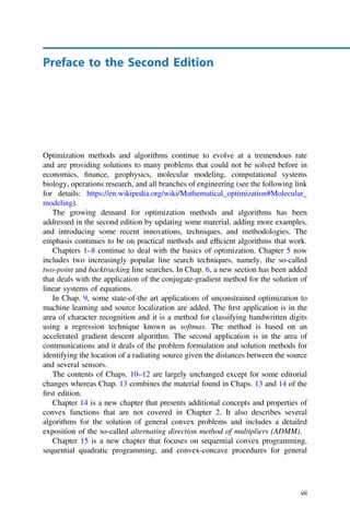
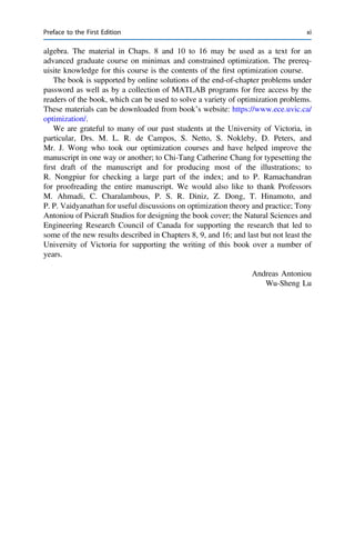
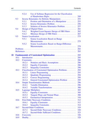
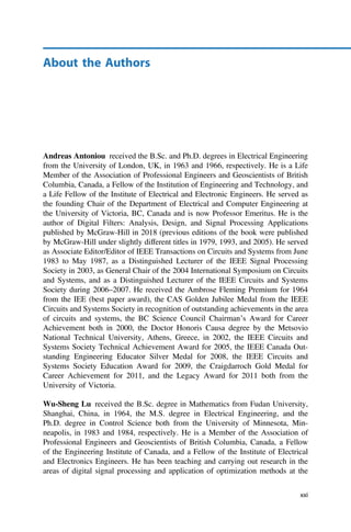
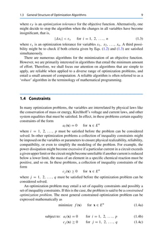
Fig.1.3 The double inverted
pendulum
θ 1
θ 2
Μ
u(t)
A problem that does not entail any equality or inequality constraints is said to be an
unconstrained optimization problem.
Constrained optimization is usually much more difficult than unconstrained opti-
mization, as might be expected. Consequently, the general strategy that has evolved
in recent years towards the solution of constrained optimization problems is to re-
formulate constrained problems as unconstrained optimization problems. This can
be done by redefining the objective function such that the constraints are simultane-
ously satisfied when the objective function is minimized. Some real-life constrained
optimization problems are given as Examples1.2 to 1.4 below.
Example 1.2 Consider a control system that comprises a double inverted pendulum
as depicted in Fig. 1.3. The objective of the system is to maintain the pendulum in the
upright position using the minimum amount of energy. This is achieved by applying
an appropriate control force to the car to damp out any displacements θ1(t) and θ2(t).
Formulate the problem as an optimization problem.
Solution The dynamic equations of the system are nonlinear and the standard practice
is to apply a linearization technique to these equations to obtain a small-signal linear
model of the system as [6]
ẋ(t) = Ax(t) + fu(t) (1.5)
where
x(t) =
⎡
⎢
⎢
⎣
θ1(t)
θ̇1(t)
θ2(t)
θ̇2(t)
⎤
⎥
⎥
⎦ , A =
⎡
⎢
⎢
⎣
0 1 0 0
α 0 −β 0
0 0 0 1
−α 0 α 0
⎤
⎥
⎥
⎦ , f =
⎡
⎢
⎢
⎣
0
−1
0
0
⎤
⎥
⎥
⎦
with α 0, β 0, and α = β. In the above equations, ẋ(t), θ̇1(t), and θ̇2(t)
represent the first derivatives of x(t), θ1(t), and θ2(t), respectively, with respect
to time, θ̈1(t) and θ̈2(t) would be the second derivatives of θ1(t) and θ2(t), and
parameters α and β depend on system parameters such as the length and weight of
each pendulum, the mass of the car, etc. Suppose that at instant t = 0 small nonzero](https://image.slidesharecdn.com/20986-250315065426-4aaea085/85/Practical-Optimization-Algorithms-and-Engineering-Applications-2nd-Edition-Andreas-Antoniou-37-320.jpg)
![1.4 Constraints 11
displacements θ1(t) and θ2(t) occur, which would call for immediate control action
in order to steer the system back to the equilibrium state x(t) = 0 at time t = T0. In
order to develop a digital controller, the system model in Eq. (1.5) is discretized to
become
x(k + 1) = x(k) + gu(k) (1.6)
where = I + ΔtA, g = Δtf, Δt is the sampling interval, and I is the identity
matrix. Let x(0) = 0 be given and assume that T0 is a multiple of Δt, i.e., T0 =
KΔt where K is an integer. We seek to find a sequence of control actions u(k) for
k = 0, 1, . . . , K − 1 such that the zero equilibrium state is achieved at t = T0, i.e.,
x(T0) = 0.
Let us assume that the energy consumed by these control actions, namely,
J =
K−1
k=0
u2
(k)
needs to be minimized. This optimal control problem can be formulated analytically
as
minimize J =
K−1
k=0
u2
(k) (1.7a)
subject to: x(K) = 0 (1.7b)
From Eq. (1.6), we know that the state of the system at t = KΔt is determined
by the initial value of the state and system model in Eq. (1.6) as
x(K) = K
x(0) +
K−1
k=0
K−k−1
gu(k)
≡ −h +
K−1
k=0
gku(k)
where h = −K x(0) and gk = K−k−1g. Hence the constraint in Eq. (1.7b) is
equivalent to
K−1
k=0
gku(k) = h (1.8)
If we define u = [u(0) u(1) · · · u(K − 1)]T and G = [g0 g1 · · · gK−1], then the
constraint in Eq. (1.8) can be expressed as Gu = h, and the optimal control problem
at hand can be formulated as the problem of finding a u that solves the minimization
problem](https://image.slidesharecdn.com/20986-250315065426-4aaea085/85/Practical-Optimization-Algorithms-and-Engineering-Applications-2nd-Edition-Andreas-Antoniou-38-320.jpg)
![12 1 The Optimization Problem
minimize uT
u (1.9a)
subject to: a(u) = 0 (1.9b)
where a(u) = Gu − h. In practice, the control actions cannot be made arbitrarily
large in magnitude. Consequently, additional constraints are often imposed on |u(i)|,
for instance,
|u(i)| ≤ m for i = 0, 1, . . . , K − 1
These constraints are equivalent to
m + u(i) ≥ 0
m − u(i) ≥ 0
Hence if we define
c(u) =
⎡
⎢
⎢
⎢
⎢
⎢
⎣
m + u(0)
m − u(0)
.
.
.
m + u(K − 1)
m − u(K − 1)
⎤
⎥
⎥
⎥
⎥
⎥
⎦
then the magnitude constraints can be expressed as
c(u) ≥ 0 (1.9c)
Obviously, the problem in Eqs. (1.9a)–(1.9c) fits nicely into the standard form of
optimization problems given by Eqs. (1.4a)–(1.4c).
Example 1.3 High performance in modern optical instruments depends on the qual-
ity of components like lenses, prisms, and mirrors. These components have reflecting
or partially reflecting surfaces, and their performance is limited by the reflectivities
of the materials of which they are made. The surface reflectivity can, however, be
altered by the deposition of a thin transparent film. In fact, this technique facilitates
the control of losses due to reflection in lenses and makes possible the construction
of mirrors with unique properties [7,8].
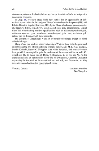
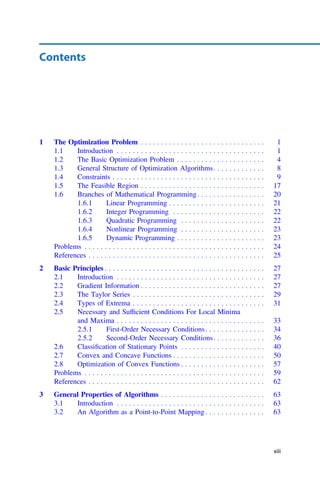
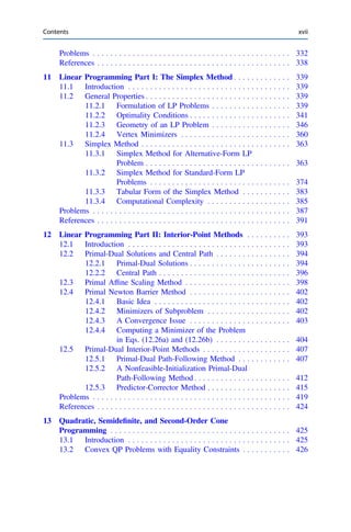
As is depicted in Fig. 1.4, a typical N-layer thin-film system consists of N layers of
thin films of certain transparent media deposited on a glass substrate. The thickness
and refractive index of the ith layer are denoted as xi and ni , respectively. The
refractive index of the medium above the first layer is denoted as n0. If φ0 is the
angle of incident light, then the transmitted ray in the (i − 1)th layer is refracted at
an angle φi which is given by Snell’s law, namely,
ni sin φi = n0 sin φ0
Given angle φ0 and the wavelength of light, λ, the energy of the light reflected
from the film surface and the energy of the light transmitted through the film surface
are usually measured by the reflectance R and transmittance T , which satisfy the
relation
R + T = 1](https://image.slidesharecdn.com/20986-250315065426-4aaea085/85/Practical-Optimization-Algorithms-and-Engineering-Applications-2nd-Edition-Andreas-Antoniou-39-320.jpg)
![1.4 Constraints 13
Fig.1.4 An N-layer
thin-film system
n0
n3
n2
nN
nN+1
layer 1
layer 2
layer 3
x2
x1 n1
Substrate
φ1
φ0
φ2
layer N xn
φN
For an N-layer system, R is given by (see [9] for details)
R(x1, . . . , xN , λ) =
η0 − y
η0 + y
2
y =
c
b
b
c
=
N
k=1
cos δk ( j sin δk)/ηk
jηk sin δk cos δk
1
ηN+1
where j =
√
−1 and
δk =
2πnk xk cos φk
λ
ηk =
⎧
⎪
⎪
⎪
⎪
⎪
⎪
⎨
⎪
⎪
⎪
⎪
⎪
⎪
⎩
nk/ cos φk for light polarized with the electric
vector lying in the plane of incidence
nk cos φk for light polarized with the electric
vector perpendicular to the
plane of incidence
The design of a multilayer thin-film system can now be accomplished as follows:
Given a range of wavelengths λl ≤ λ ≤ λu and an angle of incidence φ0, find
x1, x2, . . . , xN such that the reflectance R(x, λ) best approximates a desired re-
flectance Rd(λ) for λ ∈ [λl, λu]. Formulate the design problem as an optimization
problem.](https://image.slidesharecdn.com/20986-250315065426-4aaea085/85/Practical-Optimization-Algorithms-and-Engineering-Applications-2nd-Edition-Andreas-Antoniou-40-320.jpg)
![14 1 The Optimization Problem
Solution In practice, the desired reflectance is specified at grid points λ1, λ2, . . . , λK
in the interval [λl, λu]; hence the design may be carried out by selecting xi such
that the objective function
J =
K
i=1
wi [R(x, λi ) − Rd(λi )]2
(1.10)
is minimized, where
x = [x1 x2 · · · xN ]T
and wi 0 is a weight to reflect the importance of term [R(x, λi ) − Rd(λi )]2 in
Eq. (1.10). If we let η = [1 ηN+1]T , e+ = [η0 1]T , e− = [η0 −1]T , and
M(x, λ) =
N
k=1
cos δk ( j sin δk)/ηk
jηk sin δk cos δk
then R(x, λ) can be expressed as
R(x, λ) =
bη0 − c
bη0 + c
2
=
eT
−M(x, λ)η
eT
+M(x, λ)η
2
Finally, we note that the thickness of each layer cannot be made arbitrarily thin or
arbitrarily large and, therefore, constraints must be imposed on the elements of x as
dil ≤ xi ≤ diu for i = 1, 2, . . . , N
The design problem can now be formulated as the constrained minimization problem
minimize J =
K
i=1
wi
eT
−M(x, λi )η
eT
+M(x, λi )η
2
− Rd(λi )2
subject to: xi − dil ≥ 0 for i = 1, 2, . . . , N
diu − xi ≥ 0 for i = 1, 2, . . . , N
Example 1.4 Quantities q1, q2, . . . , qm of a certain product are produced by m
manufacturing divisions of a company, which are at distinct locations. The product
is to be shipped to n destinations that require quantities b1, b2, . . . , bn. Assume
that the cost of shipping a unit from manufacturing division i to destination j is ci j
with i = 1, 2, . . . , m and j = 1, 2, . . . , n. Find the quantity xi j to be shipped
from division i to destination j so as to minimize the total cost of transportation, i.e.,
minimize C =
m
i=1
n
j=1
ci j xi j
This is known as the transportation problem. Formulate the problem as an optimiza-
tion problem.](https://image.slidesharecdn.com/20986-250315065426-4aaea085/85/Practical-Optimization-Algorithms-and-Engineering-Applications-2nd-Edition-Andreas-Antoniou-41-320.jpg)
![1.4 Constraints 15
Solution Note that there are several constraints on variables xi j . First, each division
can provide only a fixed quantity of the product, hence
n
j=1
xi j = qi for i = 1, 2, . . . , m
Second, the quantity to be shipped to a specific destination has to meet the need of
that destination and so
m
i=1
xi j = bj for j = 1, 2, . . . , n
In addition, the variables xi j are nonnegative and thus, we have
xi j ≥ 0 for i = 1, 2, . . . , m and j = 1, 2, . . . , n
If we let
c = [c11 · · · c1n c21 · · · c2n · · · cm1 · · · cmn]T
x = [x11 · · · x1n x21 · · · x2n · · · xm1 · · · xmn]T
A =
⎡
⎢
⎢
⎢
⎢
⎢
⎢
⎢
⎢
⎢
⎢
⎣
1 1 · · · 1 0 0 · · · 0 · · · · · · · · · · · ·
0 0 · · · 0 1 1 · · · 1 · · · · · · · · · · · ·
· · · · · · · · · · · · · · · · · · · · · · · · · · · · · · · · ·
0 0 · · · 0 0 0 · · · 0 · · · 1 1 · · · 1
1 0 · · · 0 1 0 · · · 0 · · · 1 0 · · · 0
0 1 · · · 0 0 1 · · · 0 · · · 0 1 · · · 0
· · · · · · · · · · · · · · · · · · · · · · · · · · · · · · · · ·
0 0 · · · 1 0 0 · · · 1 · · · 0 0 · · · 1
⎤
⎥
⎥
⎥
⎥
⎥
⎥
⎥
⎥
⎥
⎥
⎦
b = [q1 · · · qm b1 · · · bn]T
then the minimization problem can be stated as
minimize C = cT
x (1.11a)
subject to: Ax = b (1.11b)
x ≥ 0 (1.11c)
where cT x is the inner product of c and x. The above problem, like those in Exam-
ples1.2 and 1.3, fits into the standard optimization problem in Eqs. (1.4a)–(1.4c).
Since both the objective function in Eq. (1.11a) and the constraints in Eqs. (1.11b)
and (1.11c) are linear, the problem is known as a linear programming (LP) problem
(see Sect.1.6.1).
Example 1.5 An investment portfolio is a collection of a variety of securities owned
by an individual whereby each security is associated with a unique possible return and
a corresponding risk. Design an optimal investment portfolio that would minimize
the risk involved subject to an acceptable return for a portfolio that comprises n
securities.](https://image.slidesharecdn.com/20986-250315065426-4aaea085/85/Practical-Optimization-Algorithms-and-Engineering-Applications-2nd-Edition-Andreas-Antoniou-42-320.jpg)
![16 1 The Optimization Problem
Solution Some background theory on portfolio selection can be found in [10]. As-
sume that the amount of resources to be invested is normalized to unity (e.g., 1
million dollars) and let xi represent the return of security i at some specified time in
the future, say, in one month’s time. The return xi can be assumed to be a random
variable and hence three quantities pertaining to security i can be evaluated, namely,
the expected return
μi = E[xi ]
the variance of the return
σ2
i = E[(xi − μi )2
]
and the correlation between the returns of the ith and jth securities
ρi, j =
E[(xi − μi )(x j − μj )]
σi σj
for i, j = 1, 2, . . . , n
With these quantities known, constructing a portfolio amounts to allocating a fraction
wi of the available resources to security i, for i = 1, 2, . . . , n. This leads to the
constraints
0 ≤ wi ≤ 1 for i = 1, 2, . . . , n and
n
i=1
wi = 1
Given a set of investment allocations {wi , i = 1, 2, . . . , n}, the expected return of
the portfolio can be deduced as
E
n
i=1
wi xi
=
n
i=1
wi μi
The variance for the portfolio, which measures the risk of the investment, can be
evaluated as
E
n
i=1
wi xi − E(
n
i=1
wi xi )
2
= E
⎧
⎨
⎩
n
i=1
wi (xi − μi )
⎡
⎣
n
j=1
wj (x j − μj )
⎤
⎦
⎫
⎬
⎭
= E
⎡
⎣
n
i=1
n
j=1
(xi − μi )(x j − μj )wi wj
⎤
⎦
=
n
i=1
n
j=1
E[(xi − μi )(x j − μj )]wi wj
=
n
i=1
n
j=1
(σi σj ρi j )wi wj
=
n
i=1
n
j=1
qi j wi wj
where
qi j = σi σj ρi j](https://image.slidesharecdn.com/20986-250315065426-4aaea085/85/Practical-Optimization-Algorithms-and-Engineering-Applications-2nd-Edition-Andreas-Antoniou-43-320.jpg)