Download to read offline


![Dynamic Response Surface Method
Combined with Genetic Algorithm
to Optimize Extraction Process Problem
Laires A. Lima1,2(B)
, Ana I. Pereira1
, Clara B. Vaz1
, Olga Ferreira2
,
Márcio Carocho2
, and Lillian Barros2
1
Research Center in Digitalization and Intelligent Robotics (CeDRI), Instituto
Politécnico de Bragança, Campus de Santa Apolónia, 5300-253 Bragança, Portugal
{laireslima,apereira,clvaz}@ipb.pt
2
Centro de Investigação de Montanha (CIMO), Instituto Politécnico de Bragança,
Campus de Santa Apolónia, 5300-253 Bragança, Portugal
{oferreira,mcarocho,lillian}@ipb.pt
Abstract. This study aims to find and develop an appropriate opti-
mization approach to reduce the time and labor employed throughout a
given chemical process and could be decisive for quality management. In
this context, this work presents a comparative study of two optimization
approaches using real experimental data from the chemical engineering
area, reported in a previous study [4]. The first approach is based on the
traditional response surface method and the second approach combines
the response surface method with genetic algorithm and data mining.
The main objective is to optimize the surface function based on three
variables using hybrid genetic algorithms combined with cluster analysis
to reduce the number of experiments and to find the closest value to
the optimum within the established restrictions. The proposed strategy
has proven to be promising since the optimal value was achieved with-
out going through derivability unlike conventional methods, and fewer
experiments were required to find the optimal solution in comparison to
the previous work using the traditional response surface method.
Keywords: Optimization · Genetic algorithm · Cluster analysis
1 Introduction
Search and optimization methods have several principles, being the most rele-
vant: the search space, where the possibilities for solving the problem in question
are considered; the objective function (or cost function); and the codification of
the problem, that is, the way to evaluate an objective in the search space [1].
Conventional optimization techniques start with an initial value or vector
that, iteratively, is manipulated using some heuristic or deterministic process
c
Springer Nature Switzerland AG 2021
A. I. Pereira et al. (Eds.): OL2A 2021, CCIS 1488, pp. 3–14, 2021.
https://doi.org/10.1007/978-3-030-91885-9_1](https://image.slidesharecdn.com/optimizationlearningalgorithmsandapplications-231204021346-9e8015c0/85/Optimization-Learning-Algorithms-and-Applications-pdf-16-320.jpg)
![4 L. A. Lima et al.
directly associated with the problem to be solved. The great difficulty to deal
with when solving a problem using a stochastic method is the number of possible
solutions growing with a factorial speed, being impossible to list all possible
solutions of the problem [12]. Evolutionary computing techniques operate on a
population that changes in each iteration. Thus, they can search in different
regions on the feasible space, allocating an appropriate number of members to
search in different areas [12].
Considering the importance of predicting the behavior of analytical processes
and avoiding expensive procedures, this study aims to propose an alternative
for the optimization of multivariate problems, e.g. extraction processes of high-
value compounds from plant matrices. In the standard analytical approach, the
identification and quantification of phenolic compounds require expensive and
complex laboratory assays [6]. An alternative approach can be applied using
forecasting models from Response Surface Method (RSM). This approach can
maximize the extraction yield of the target compounds while decreasing the cost
of the extraction process.
In this study, a comparative analysis between two optimization methodolo-
gies (traditional RSM and dynamic RSM), developed in MATLAB R
software
(version R2019a 9.6), that aim to maximize the heat-assisted extraction yield
and phenolic compounds content in chestnut flower extracts is presented.
This paper is organized as follows. Section 2 describes the methods used to
evaluate multivariate problems involving optimization processes: Response Sur-
face Method (RSM), Hybrid Genetic Algorithm, Cluster Analysis and Bootsrap
Analysis. Sections 3 and 4 introduce the case study, consisting of the optimization
of the extraction yield and content of phenolic compounds in extracts of chest-
nut flower by two different approaches: Traditional RSM and Dynamic RSM.
Section 5 includes the numerical results obtained by both methods and their
comparative evaluation. Finally, Sect. 6 presents the conclusions and future work.
2 Methods Approaches and Techniques
Regarding optimization problems, some methods are used more frequently (tra-
ditional RSM, for example) due to their applicability and suitability to different
cases. For the design of the dynamic RSM, the approach of conventional meth-
ods based on Genetic Algorithm combined with clustering and bootstrap analysis
was made to evaluate the aspects that could be incorporated into the algorithm
developed in this work. The key concepts for dynamic RSM are presented below.
2.1 Response Surface Method
The Response Surface Method is a tool introduced in the early 1950s by Box
and Wilson, which covers a collection of mathematical and statistical techniques
useful for approximating and optimizing stochastic models [11]. It is a widely
used optimization method, which applies statistical techniques based on special
factorial designs [2,3]. Its scientific approach estimates the ideal conditions for](https://image.slidesharecdn.com/optimizationlearningalgorithmsandapplications-231204021346-9e8015c0/85/Optimization-Learning-Algorithms-and-Applications-pdf-17-320.jpg)
![Dynamic RSM Combined with GA to Optimize Extraction Process Problem 5
achieving the highest or lowest required response value, through the design of the
response surface from the Taylor series [8]. RSM promotes the greatest amount
of information on experiments, such as the time of experiments and the influence
of each dependent variable, being one of the largest advantages in obtaining the
necessary general information on the planning of the process and the experience
design [8].
2.2 Hybrid Genetic Algorithm
The genetic algorithm is a stochastic optimization method based on the evolu-
tionary process of natural selection and genetic dynamics. The method seeks to
combine the survival of the fittest among the string structures with an exchange
of random, but structured, information to form an ideal solution [7]. Although
they are randomized, GA search strategies are able to explore several regions
of the feasible search space at a time. In this way, along with the iterations,
a unique search path is built, as new solutions are obtained through the com-
bination of previous solutions [1]. Optimization problems with restrictions can
influence the sampling capacity of a genetic algorithm due to the population
limits considered. Incorporating a local optimization method into GA can help
overcome most of the obstacles that arise as a result of finite population sizes,
for example, the accumulation of stochastic errors that generate genetic drift
problems [1,7].
2.3 Cluster Analysis
Cluster algorithms are often used to group large data sets and play an impor-
tant role in pattern recognition and mining large arrays. k-means and k-medoids
strategies work by grouping partition data into a k number of mutually exclusive
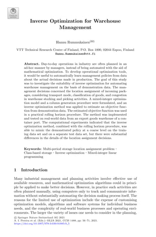
clusters, demonstrated in Fig. 1. These techniques assign each observation to a
cluster, minimizing the distance from the data point to the average (k-means)
or median (k-medoids) location of its assigned cluster [10].
Fig. 1. Mean and Medoid in 2D space representation. In both figures, the data are
represented by blue dots, being the rightmost point an outlier and the red point rep-
resents the centroid point found by k-mean or k-medoid methods. Adapted from Jin
and Han (2011) (Color figure online).](https://image.slidesharecdn.com/optimizationlearningalgorithmsandapplications-231204021346-9e8015c0/85/Optimization-Learning-Algorithms-and-Applications-pdf-18-320.jpg)
![6 L. A. Lima et al.
2.4 Bootstrap Analysis
The idea of bootstrap analysis is to mimic the sampling distribution of the statis-
tic of interest through the use of many resamples replacing the original sample
elements [5]. In this work, the bootstrap analysis enables the handling of the vari-
ability of the optimal solutions derived from the cluster method analysis. Thus,
the bootstrap analysis is used to estimate the confidence interval of the statis-
tic of interest and subsequently, comparing the results obtained by traditional
methods.
3 Case Study
This work presents a comparative analysis between two methodologies for opti-
mizing the total phenolic content in extracts of chestnut flower, developed in
MATLAB R
software. The natural values of the dependent variables in the
extraction - t, time in minutes; T, temperature in ◦
C; and S, organic solvent con-
tent in %v/v of ethanol - were coded based on Central Composite Circumscribed
Design (CCCD) and the result was based on extraction yield (Y, expressed in
percentage of dry extract) and total phenolic content (Phe, expressed in mg/g
of dry extract) as shown in Table 1.
The experimental data presented were cordially provided by the Mountain
Research Center - CIMO (Bragança, Portugal) [4].
The CCCD design selected for the original experimental study [4] is based
on a cube circumscribed to a sphere in which the vertices are at α distance from
the center, with 5 levels for each factor (t, T, and S). In this case, the α values
vary between −1.68 and 1.68, and correspond to each factor level, as described
in Table 2.
4 Data Analysis
In this section, the two RSM optimization methods (traditional and dynamic)
will be discussed in detail, along with the results obtained from both methods.
4.1 Traditional RSM
In the original experiment, a five-level Central Composite Circumscribed Design
(CCCD) coupled with RSM was build to optimize the variables for the male
chestnut flowers. For the optimization, a simplex method developed ad hoc was
used to optimize nonlinear solutions obtained by a regression model to maximize
the response, described in the flowchart in Fig. 2.
Through the traditional RSM, the authors approximated the surface response
to a second-order polynomial function [4]:
Y = b0 +
n
i=1
biXi +
n−1
i=1
j1
n
j=2
bijXiXj +
n
i=1
biiX2
i (1)](https://image.slidesharecdn.com/optimizationlearningalgorithmsandapplications-231204021346-9e8015c0/85/Optimization-Learning-Algorithms-and-Applications-pdf-19-320.jpg)
![Dynamic RSM Combined with GA to Optimize Extraction Process Problem 7
Table 1. Variables and natural values of the process parameters for the extraction of
chestnut flowers [4].
t (min) T (◦
C) S (%EtOH) Yield (%R) Phenolic cont.
(mg.g−1
dry weight)
40.30 37.20 20.30 38.12 36.18
40.30 37.20 79.70 26.73 11.05
40.30 72.80 20.30 42.83 36.66
40.30 72.80 79.70 35.94 22.09
99.70 37.20 20.30 32.77 35.55
99.70 37.20 79.70 32.99 8.85
99.70 72.80 20.30 42.55 29.61
99.70 72.80 79.70 35.52 11.10
120.00 55.00 50.00 42.41 14.56
20.00 55.00 50.00 35.45 24.08
70.00 25.00 50.00 38.82 12.64
70.00 85.00 50.00 42.06 17.41
70.00 55.00 0.00 35.24 34.58
70.00 55.00 100.00 15.61 12.01
20.00 25.00 0.00 22.30 59.56
20.00 25.00 100.00 8.02 15.57
20.00 85.00 0.00 34.81 42.49
20.00 85.00 100.00 18.71 50.93
120.00 25.00 0.00 31.44 40.82
120.00 25.00 100.00 15.33 8.79
120.00 85.00 0.00 34.96 45.61
120.00 85.00 100.00 32.70 21.89
70.00 55.00 50.00 41.03 14.62
Table 2. Natural and coded values of the extraction variables [4].
Natural variables Coded value
t (min) T (◦
C) S (%)
20.0 25.0 0.0 −1.68
40.3 37.2 20.0 −1.00
70 55 50.0 0.00
99.7 72.8 80.0 1.00
120 85 100.0 1.68](https://image.slidesharecdn.com/optimizationlearningalgorithmsandapplications-231204021346-9e8015c0/85/Optimization-Learning-Algorithms-and-Applications-pdf-20-320.jpg)
![8 L. A. Lima et al.
Fig. 2. Flowchart of traditional RSM modeling approach for optimal design.
where, for i = 0, ..., n and j = 1, ..., n, bi stand for the linear coefficients; bij
correspond to the interaction coefficients while bii are the quadratic coefficients;
and, finally, Xi are the independent variables, associated to t, T and S, being n
the total number of variables.
In the previous study, the traditional RSM, Eq. 1 represents coherently the
behaviour of the extraction process of the target compounds from chestnut flow-
ers [4]. In order to compare the optimization methods and to avoid data conflict,
the estimation of the cost function was done based on a multivariate regression
model.
4.2 Dynamic RSM
For the proposed optimization method, briefly described in the flowchart shown
in Fig. 3, the structure of the design of the experience was maintained, as well
as the imposed restrictions on the responses and variables to elude awkward
solutions.
Fig. 3. Flowchart of dynamic RSM integrating genetic algorithm and cluster analysis
to the process.
The dynamic RSM method was build in MATLAB R
using a programming
code developed by the authors coupled with pre-existing functions from the
statistical and optimization toolboxes of the software. The algorithm starts by
generating a set of 15 random combinations between the levels of combinatorial
analysis. From this initial experimental data, a multivariate regression model is
calculated, being this model the objective function of the problem. Thereafter,
a built-in GA-based solver was used to solve the optimization problem. The
optimal combination is identified and it is used to define the objective function.
The process stops when no new optimal solution is identified.](https://image.slidesharecdn.com/optimizationlearningalgorithmsandapplications-231204021346-9e8015c0/85/Optimization-Learning-Algorithms-and-Applications-pdf-21-320.jpg)
![Dynamic RSM Combined with GA to Optimize Extraction Process Problem 9
Considering the stochastic nature of this case study, clustering analysis is
used to identify the best candidate optimal solution. In order to handle the
variability of the achieved optimal solution, the bootstrap method is used to
estimate the confidence interval at 95%.
5 Numerical Results
The study using the traditional RSM returned the following optimal conditions
for maximum yield: 120.0 min, 85.0 ◦
C, and 44.5% of ethanol in the solvent, pro-
ducing 48.87% of dry extract. For total phenolic content, the optimal conditions
were: 20.0 min, 25.0 ◦
C and S = 0.0% of ethanol in the solvent, producing 55.37
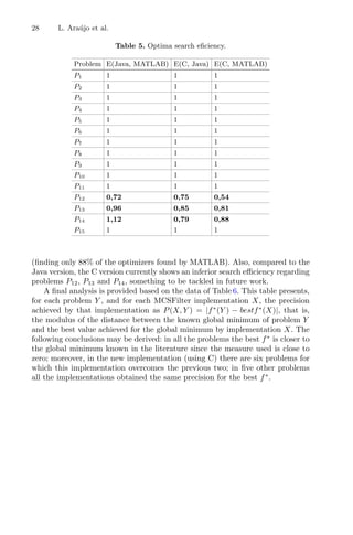
mg/g of dry extract. These data are displayed in Table 3.
Table 3. Optimal responses and respective conditions using traditional and dynamic
RSM based on confidence intervals at 95%.
Method t (min) T (◦
C) S (%) Response
Extraction yield (%) Traditional RSM 120.0 ± 12.4 85.0 ± 6.7 44.5 ± 9.7 48.87
Dynamic RSM 118.5 ± 1.4 84.07 ± 0.9 46.1 ± 0.85 45.87
Total phenolics (Phe) Traditional RSM 20.0 ± 3.7 25.0 ± 5.7 0.0 ± 8.7 55.37
Dynamic RSM 20.4 ± 1.5 25.1 ± 1.97 0.05 ± 0.05 55.64
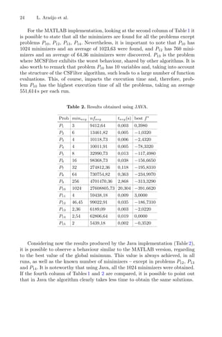
For the implementation of dynamic RSM in this case study, 100 runs were
carried out to evaluate the effectiveness of the method. For the yield, the esti-
mated optimal conditions were: 118.5 min, 84.1 ◦
C, and 46.1% of ethanol in the
solvent, producing 45.87% of dry extract. In this case, the obtained optimal con-
ditions for time and temperature were in accordance with approximately 80% of
the tests.
For the total phenolic content, the optimal conditions were: 20.4 min, 25.1
◦
C, and 0.05% of ethanol in the solvent, producing 55.64 mg/g of dry extract.
The results were very similar to the previous report with the same data [4].
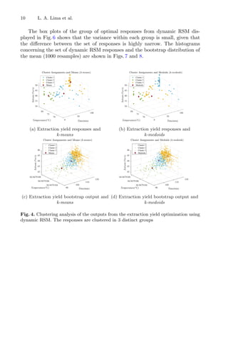
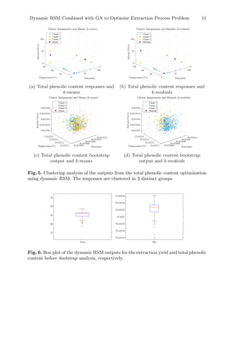
The clustering analysis for each response variable was performed considering
the means (Figs. 4a and 5a) and the medoids (Figs. 4b and 5b) for the output
population (optimal responses). The bootstrap analysis makes the inference con-
cerning the results achieved and are represented graphically in terms of mean in
Figs. 4c and 5c, and in terms of medoids in Figs. 4d and 5d.](https://image.slidesharecdn.com/optimizationlearningalgorithmsandapplications-231204021346-9e8015c0/85/Optimization-Learning-Algorithms-and-Applications-pdf-22-320.jpg)
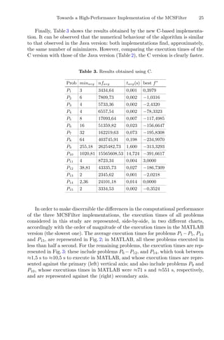
![12 L. A. Lima et al.
Fig. 7. Histograms of the extraction data (extraction yield) and the bootstrap means,
respectively.
Fig. 8. Histograms of the extraction data (total phenolic content) and the bootstrap
means, respectively.
The results obtained in this work are satisfactory since they were analogous
for both methods, although dynamic RSM took 15 to 18 experimental points
to find the optimal coordinates. Some authors use the design of experiments
involving traditional RSM containing 20 different combinations, including the
repetition of centroid [4]. However, in studies involving recent data or the absence
of complementary data, evaluations about the influence of parameters and range
are essential to obtain consistent results, making it necessary to make about 30
experimental points for optimization. Considering these cases, the dynamic RSM
method proposes a different, competitive, and economical approach, in which
fewer points are evaluated to obtain the maximum response.
Genetic algorithms have been providing their efficiency in the search for
optimal solutions in a wide variety of problems, given that they do not have
some limitations found in traditional search methodologies, such as the require-
ment of the derivative function, for example [9]. GA is attractive to identify the
global solution of the problem. Considering the stochastic problem presented in
this work, the association of genetic algorithm with the k-methods as clustering
algorithm obtained satisfactory results. This solution can be used for problems
involving small-scale data since GA manages to gather the best data for opti-](https://image.slidesharecdn.com/optimizationlearningalgorithmsandapplications-231204021346-9e8015c0/85/Optimization-Learning-Algorithms-and-Applications-pdf-25-320.jpg)
![Dynamic RSM Combined with GA to Optimize Extraction Process Problem 13
mization through its evolutionary method, while k-means or k-medoids make the
grouping of optimum points.
In addition to clustering analysis, bootstrapping was also applied, in which
the sample distribution of the statistic of interest is simulated through the use
of many resamples with replacement of the original sample, thus enabling to
make the statistical inference. Bootstrapping was used to calculate the confidence
intervals to obtain unbiased estimates from the proposed method. In this case,
the confidence interval was calculated at the 95% level (two-tailed), since the
same percentage was adopted by Caleja et al. (2019). It was observed that the
Dynamic RSM approach also enables the estimation of confidence intervals with
less margin of error than the Traditional RSM approach, conducting to define
more precisely the optimum conditions for the experiment.
6 Conclusion and Future Work
For the presented case study, applying dynamic RSM using Genetic Algorithm
coupled with clustering analysis returned positive results, in accordance with
previous published data [4]. Both methods seem attractive for the resolution
of this particular case concerning the optimization of the extraction of target
compounds from plant matrices. Therefore, the smaller number of experiments
required for dynamic RSM can be an interesting approach for future studies.
In brief, a smaller set of points was obtained that represent the best domain
of optimization, thus eliminating the need for a large number of costly labora-
tory experiments. The next steps involve the improvement of the dynamic RSM
algorithm and the application of the proposed method in other areas of study.
Acknowledgments. The authors are grateful to FCT for financial support through
national funds FCT/MCTES UIDB/00690/2020 to CIMO and UIDB/05757/2020.
M. Carocho also thanks FCT through the individual scientific employment program-
contract (CEECIND/00831/2018).
References
1. Beasley, D., Bull, D.R., Martin, R.R.: An overview of genetic algorithms: Part 1,
fundamentals. Univ. Comput. 2(15), 1–16 (1993)
2. Box, G.E.P., Behnken, D.W.: Simplex-sum designs: a class of second order rotatable
designs derivable from those of first order. Ann. Math. Stat. 31(4), 838–864 (1960)
3. Box, G.E.P., Wilson, K.B.: On the experimental attainment of optimum conditions.
J. Roy. Stat. Soc. Ser. B (Methodol.) 13(1), 1–38 (1951)
4. Caleja C., Barros L., Prieto M. A., Bento A., Oliveira M.B.P., Ferreira, I.C.F.R.:
Development of a natural preservative obtained from male chestnut flowers: opti-
mization of a heat-assisted extraction technique. In: Food and Function, vol. 10,
pp. 1352–1363 (2019)
5. Efron, B., Tibshirani, R.J.: An introduction to the Bootstrap, 1st edn. Wiley, New
York (1994)](https://image.slidesharecdn.com/optimizationlearningalgorithmsandapplications-231204021346-9e8015c0/85/Optimization-Learning-Algorithms-and-Applications-pdf-26-320.jpg)

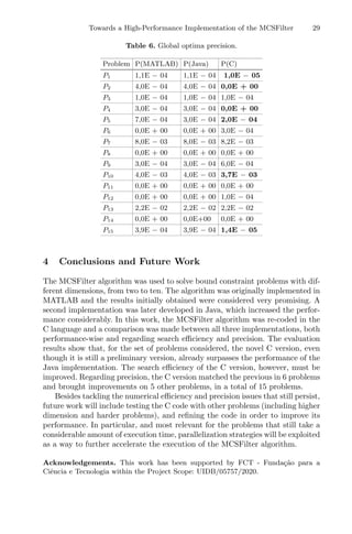
![Towards a High-Performance
Implementation of the MCSFilter
Optimization Algorithm
Leonardo Araújo1,2
, Maria F. Pacheco2
, José Rufino2
,
and Florbela P. Fernandes2(B)
1
Universidade Tecnológica Federal do Paraná,
Campus de Ponta Grossa, Ponta Grossa 84017-220, Brazil
2
Research Centre in Digitalization and Intelligent Robotics (CeDRI),
Instituto Politécnico de Bragança, 5300-252 Bragança, Portugal
a46677@alunos.ipb.pt, {pacheco,rufino,fflor}@ipb.pt
Abstract. Multistart Coordinate Search Filter (MCSFilter) is an opti-
mization method suitable to find all minimizers – both local and global –
of a non convex problem, with simple bounds or more generic constraints.
Like many other optimization algorithms, it may be used in industrial
contexts, where execution time may be critical in order to keep a pro-
duction process within safe and expected bounds. MCSFilter was first
implemented in MATLAB and later in Java (which introduced a signif-
icant performance gain). In this work, a comparison is made between
these two implementations and a novel one in C that aims at further
performance improvements. For the comparison, the problems addressed
are bound constraint, with small dimension (between 2 and 10) and mul-
tiple local and global solutions. It is possible to conclude that the average
time execution for each problem is considerable smaller when using the
Java and C implementations, and that the current C implementation,
though not yet fully optimized, already exhibits a significant speedup.
Keywords: Optimization · MCSFilter method · MatLab · C · Java ·
Performance
1 Introduction
The set of techniques and principals for solving quantitative problems known as
optimization has become increasingly important in a broad range of applications
in areas of research as diverse as engineering, biology, economics, statistics or
physics. The application of the techniques and laws of optimization in these
(and other) areas, not only provides resources to describe and solve the specific
problems that appear within the framework of each area but it also provides the
opportunity for new advances and achievements in optimization theory and its
techniques [1,2,6,7].
c
Springer Nature Switzerland AG 2021
A. I. Pereira et al. (Eds.): OL2A 2021, CCIS 1488, pp. 15–30, 2021.
https://doi.org/10.1007/978-3-030-91885-9_2](https://image.slidesharecdn.com/optimizationlearningalgorithmsandapplications-231204021346-9e8015c0/85/Optimization-Learning-Algorithms-and-Applications-pdf-28-320.jpg)
![16 L. Araújo et al.
In order to apply optimization techniques, problems can be formulated in
terms of an objective function that is to be maximized or minimized, a set of
variables and a set of constraints (restrictions on the values that the variables can
assume). The structure of the these three items – objective function, variables
and constraints –, determines different subfields of optimization theory: linear,
integer, stochastic, etc.; within each of these subfields, several lines of research
can be pursued. The size and complexity of optimization problems that can be
dealt with has increased enormously with the improvement of the overall per-
formance of computers. As such, advances in optimization techniques have been
following progresses in computer science as well as in combinatorics, operations
research, control theory, approximation theory, routing in telecommunication
networks, image reconstruction and facility location, among other areas [14].
The need to keep up with the challenges of our rapidly changing society and
its digitalization means a continuing need to increase innovation and productiv-
ity and improve the performance of the industry sector, and places very high
expectations for the progress and adaptation of sophisticated optimization tech-
niques that are applied in the industrial context. Many of those problems can be
modelled as nonlinear programming problems [10–12] or mixed integer nonlinear
programming problems [5,8]. The urgency to quickly output solutions to difficult
multivariable problems, leads to an increasing need to develop robust and fast
optimization algorithms. Considering that, for many problems, reliable informa-
tion about the derivative of the objective function is unavailable, it is important
to use a method that allows to solve the problem without this information.
Algorithms that do not use derivatives are called derivative-free. The MCS-
Filter method is such a method, being able to deal with discontinuous or non-
differentiable functions that often appear in many applications. It is also a multi-
local method, meaning that it finds all the minimizers, both local and global, and
exhibits good results [9,10]. Moreover, a Java implementation was already used
to solve processes engineering problems [4]. Considering that, from an industrial
point of view, execution time is of utmost importance, a novel C reimplementa-
tion, aimed at increased performance, is currently under way, having reached a
stage at which it is already able to solve a broad set of problems with measur-
able performance gains over the previous Java version. This paper presents the
results of a preliminary evaluation of the new C implementation of the MCSFilter
method, against the previously developed versions (in MATLAB and Java).
The rest of this paper is organized as follows: in Sect. 2, the MCSFilter algo-
rithm is briefly described; in Sect. 3 the set of problems that are used to compare
the three implementations and the corresponding results are presented and ana-
lyzed. Finally, in Sect. 4, conclusions and future work are addressed.
2 The Multistart Coordinate Search Filter Method
The MCSFilter algorithm was initially developed in [10], with the aim of finding
multiple solutions of nonconvex and nonlinear constrained optimization problems
of the following type:](https://image.slidesharecdn.com/optimizationlearningalgorithmsandapplications-231204021346-9e8015c0/85/Optimization-Learning-Algorithms-and-Applications-pdf-29-320.jpg)
![Towards a High-Performance Implementation of the MCSFilter 17
min f(x)
subject to gj(x) ≤ 0, j = 1, ..., m
li ≤ xi ≤ ui, i = 1, ..., n
(1)
where f is the objective function, gj(x), j = 1, ..., m are the constraint functions
and at least one of the functions f, gj : Rn
−→ R is nonlinear; also, l and u are
the bounds and Ω = {x ∈ Rn
: g(x) ≤ 0 , l ≤ x ≤ u} is the feasible region.
This method has two main different parts: i) the multistart part, related with
the exploration feature of the method, and ii) the coordinate search filter local
search, related with the exploitation of promising regions.
The MCSFilter method does not require any information about the deriva-
tives and is able to obtain all the solutions, both local and global, of a given non-
convex optimization problem. This is an important asset of the method since,
in industry problems, it is often not possible to know the derivative functions;
moreover, a large number of real-life problems are nonlinear and nonconvex.
As already stated, the MCSFilter algorithm relies on a multistart strategy
and a local search repeatedly called inside the multistart. Briefly, the multistart
strategy is a stochastic algorithm that applies more than once a local search to
sample points aiming to converge to all the minimizers, local and global, of a
multimodal problem. When the local search is repeatedly applied, some of the
minimizers can be reached more than once. This leads to a waste of time since
these minimizers have already been determined. To avoid these situations, a
clustering technique based on computing the regions of attraction of previously
identified minimizers is used. Thus, if the initial point belongs to the region of
attraction of a previously detected minimizer, the local search procedure may
not be performed, since it would converge to this known minimizer.
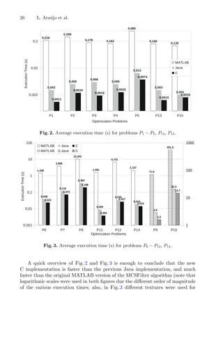
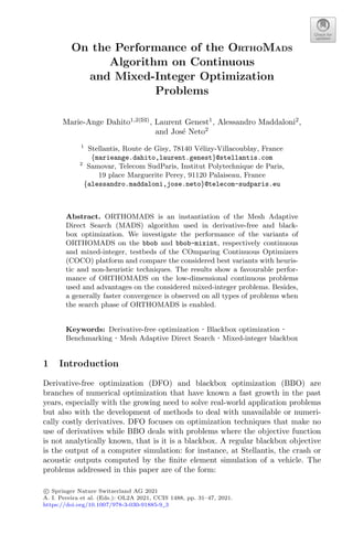
Figure 1 illustrates the influence of the regions of attraction. The red/magenta
lines between the initial approximation and the minimizer represent a local
search that has been performed; the red line represents the first local search that
converged to a given minimizer; the white dashed line between the two points
represents a discarded local search, using the regions of attraction. Therefore,
this representation intends to show the regions of attraction of each minimizer
and the corresponding points around each one. These regions are dynamic in the
sense that they may change every time a new initial point is used [3].
The local search uses a derivative-free strategy that consists of a coordinate
search combined with a filter methodology in order to generate a sequence of
approximate solutions that improve either the constraint violation or the objec-
tive function relatively to the previous approximation; this strategy is called
Coordinate Search Filter algorithm (CSFilter). In this way, the initial problem
is previously rewritten as a bi-objective problem (2):
min (θ(x), f(x))
x ∈ Ω
(2)](https://image.slidesharecdn.com/optimizationlearningalgorithmsandapplications-231204021346-9e8015c0/85/Optimization-Learning-Algorithms-and-Applications-pdf-30-320.jpg)
![18 L. Araújo et al.
3 4 5 6 7 8 9 10 11 12 13
3
4
5
6
7
8
9
10
11
12
13
Fig. 1. Illustration of the multistart strategy with regions of attraction [3].
aiming to minimize, simultaneously, the objective function f(x) and the non-
negative continuous aggregate constraint violation function θ(x) defined in (3):
θ(x) = g(x)+2
+ (l − x)+2
+ (x − u)+2
(3)
where v+ = max{0, v}. For more details about this method see [9,10].
Algorithm 1 displays the steps of the MSCFilter method. The stopping condi-
tion of CSFilter is related with the step size α of the method (see condition (4)):
α αmin (4)
with αmin 1 and close to zero.
The main steps of the MCSFilter algorithm for finding global (as well as
local) solutions to problem (1) are shown in Algorithm 2.
The stopping condition of the MCSFilter algorithm is related to the number
of minimizers found and to the number of local searches that were applied in
the multistart strategy. Considering nl as the number of local searches used
and nm as the number of minimizers obtained, then Pmin =
nm(nm + 1)
nl(nl − 1)
. The
MCSFilter algorithm stops when condition (5) is reached:
Pmin (5)
where 1.
In this preliminary work, the main goal is to compare the performance
of MCSFilter when bound constraint problems are addressed, using different](https://image.slidesharecdn.com/optimizationlearningalgorithmsandapplications-231204021346-9e8015c0/85/Optimization-Learning-Algorithms-and-Applications-pdf-31-320.jpg)
![Towards a High-Performance Implementation of the MCSFilter 19
Algorithm 1. CSFilter algorithm
Require: x and parameter values, αmin; set x̃ = x, xinf
F = x, z = x̃;
1: Initialize the filter; Set α = min{1, 0.05
n
i=1 ui−li
n
};
2: repeat
3: Compute the trial approximations zi
a = x̃ + αei, for all ei ∈ D⊕;
4: repeat
5: Check acceptability of trial points zi
a;
6: if there are some zi
a acceptable by the filter then
7: Update the filter;
8: Choose zbest
a ; set z = x̃, x̃ = zbest
a ; update xinf
F if appropriate;
9: else
10: Compute the trial approximations zi
a = xinf
F + αei, for all ei ∈ D⊕;
11: Check acceptability of trial points zi
a;
12: if there are some zi
a acceptable by the filter then
13: Update the filter;
14: Choose zbest
a ; Set z = x̃, x̃ = zbest
a ; update xinf
F if appropriate;
15: else
16: Set α = α/2;
17: end if
18: end if
19: until new trial zbest
a is acceptable
20: until α αmin
implementations of the algorithm: the original implementation in MATLAB [10],
a follow up implementation in Java (already used to solve problems from the
Chemical Engineering area [3,4,13]), and a new implementation in C (evaluated
for the first time in this paper).
3 Computational Results
In order to compare the performance of the three implementations of the MCS-
Filter optimization algorithm, a set of problems was chosen. The definition of
each problem (a total of 15 bound constraint problems) is given below, along
with the experimental conditions under which they were evaluated, as well as
the obtained results (both numerical and performance-related).
3.1 Benchmark Problems
The collection of problems was taken from [9] (and the references therein) and
all the fifteen problems in study are listed below. The problems were chosen in
such a way that different characteristics were addressed: they are multimodal
problems with more than one minimizer (actually, the number of minimizers
varies from 2 to 1024); they can have just one global minimizer or more than
one global minimizer; the dimension of the problems varies between 2 and 10.](https://image.slidesharecdn.com/optimizationlearningalgorithmsandapplications-231204021346-9e8015c0/85/Optimization-Learning-Algorithms-and-Applications-pdf-32-320.jpg)
![20 L. Araújo et al.
Algorithm 2. MCSFilter algorithm
Require: Parameter values; set M∗
= ∅, k = 1, t = 1;
1: Randomly generate x ∈ [l, u]; compute Bmin = mini=1,...,n{ui − li};
2: Compute m1 = CSFilter(x), R1 = x − m1; set r1 = 1, M∗
= M∗
∪ m1;
3: while the stopping rule is not satisfied do
4: Randomly generate x ∈ [l, u];
5: Set o = arg minj=1,...,k dj ≡ x − mj;
6: if do Ro then
7: if the direction from x to yo is ascent then
8: Set prob = 1;
9: else
10: Compute prob = φ( do
Ro
, ro);
11: end if
12: else
13: Set prob = 1;
14: end if
15: if ζ‡
prob then
16: Compute m = CSFilter(x); set t = t + 1;
17: if m − mj γ∗
Bmin, for all j = 1, . . . , k then
18: Set k = k + 1, mk = m, rk = 1, M∗
= M∗
∪ mk; compute Rk = x − mk;
19: else
20: Set Rl = max{Rl, x − ml}; rl = rl + 1;
21: end if
22: else
23: Set Ro = max{Ro, x − mo}; ro = ro + 1;
24: end if
25: end while
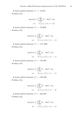
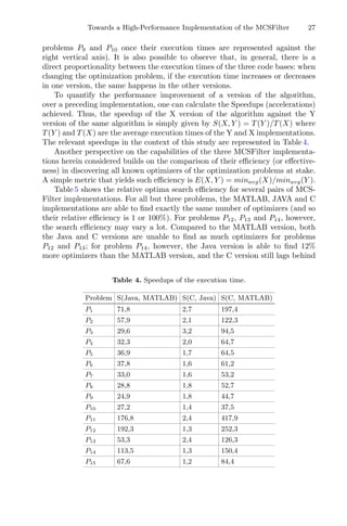
– Problem (P1)
min f(x) ≡
x2 −
5.1
4π2
x2
1 +
5
π
x1 − 6
2
+ 10
1 −
1
8π
cos(x1) + 10
s.t. −5 ≤ x1 ≤ 10, 0 ≤ x2 ≤ 15
• known global minimum f∗
= 0.39789.
– Problem (P2)
min f(x) ≡
4 − 2.1x2
1 +
x4
1
3
x2
1 + x1x2 − 4(1 − x2
2)x2
2
s.t. −2 ≤ xi ≤ 2, i = 1, 2
• known global minimum: f∗
= −1.03160.
– Problem (P3)
min f(x) ≡
n
i=1
sin(xi) + sin
2xi
3
s.t. 3 ≤ xi ≤ 13, i = 1, 2](https://image.slidesharecdn.com/optimizationlearningalgorithmsandapplications-231204021346-9e8015c0/85/Optimization-Learning-Algorithms-and-Applications-pdf-33-320.jpg)


![32 M.-A. Dahito et al.
minimize
x∈X
f(x), (1)
where X is a bounded domain of either Rn
or Rc
× Zi
with c and i respectively
the number of continuous and integer variables. n = c+i is the dimension of the
problem and f is a blackbox function. Heuristic and non-heuristic techniques
can tackle this kind of problems. Among the main approaches used in DFO
are direct local search methods. The latter are iterative methods that, at each
iteration, evaluate a set of points in a certain radius that can be increased if a
better solution is found or decreased if the incumbent remains the best point at
the current iteration.
The Mesh Adaptive Direct Search (MADS) [1,4,5] is a famous direct local
search method used in DFO and BBO that is an extension of the Generalized
Pattern Search (GPS) introduced in [28]. MADS evolves on a mesh by first doing
a global exploration called the search phase and then, if a better solution than
the current iterate is not found, a local poll is performed. The points evaluated
in the poll are defined by a finite set of poll directions that is updated at each
iteration. The algorithm is derived in several instantiations available in the Non-
linear Optimization with the MADS algorithm (NOMAD) software [7,19] and
its performance is evaluated in several papers. As examples, a broad compar-
ison of DFO optimizers is performed on 502 problems in [25] and NOMAD is
used in [24] with a DACE surrogate and compared with other local and global
surrogate-based approaches in the context of constrained blackbox optimization
on an automotive optimization problem and twenty two test problems.
Given the growing number of algorithms to deal with BBO problems, the
choice of the most adapted method for solving a specific problem still remains
complex. In order to help with this decision, some tools have been developed
to compare the performance of algorithms. In particular, data profiles [20] are
frequently used in DFO and BBO to benchmark algorithms: they show, given
some precision or target value, the fraction of problems solved by an algorithm
according to the number of function evaluations. There also exist suites of aca-
demic test problems: although the latter are treated as blackbox functions, they
are analytically known, which is an advantage to understand the behaviour of
an algorithm. There are also available industrial applications but they are rare.
Twenty two implementations of derivative-free algorithms for solving box-
constrained optimization problems are benchmarked in [25] and compared with
each other according to different criteria. They use a set of 502 problems that
are categorized according to their convexity (convex or nonconvex), smoothness
(smooth or non-smooth) and dimensions between 1 and 300. The algorithms
tested include local-search methods such as MADS through NOMAD version
3.3 and global-search methods such as the NEW Unconstrained Optimization
Algorithm (NEWUOA) [23] using trust regions and the Covariance Matrix Adap-
tation - Evolution Strategy (CMA-ES) [16] which is an evolutionary algorithm.
Simulation optimization deals with problems where at least some of the objec-
tive or constraints come from stochastic simulations. A review of algorithms to
solve simulation optimization is presented in [2], among which the NOMAD
software. However, this paper does not compare them due to a lack of standard
comparison tools and large-enough testbeds in this optimization branch.](https://image.slidesharecdn.com/optimizationlearningalgorithmsandapplications-231204021346-9e8015c0/85/Optimization-Learning-Algorithms-and-Applications-pdf-45-320.jpg)
![ORTHOMADS on Continuous and Mixed-Integer Optimization Problems 33
In [3], the MADS algorithm is used to optimize the treatment process of
spent potliners in the production of aluminum. The problem is formalized as
a 7–dimensional non-linear blackbox problem with 4 inequality constraints. In
particular, three strategies are compared using absolute displacements, relative
displacements and the latter with a global Latin hypercube sampling search.
They show that the use of scaling is particularly beneficial on the considered
chemical application.
The instantiation ORTHOMADS is introduced in Ref. [1] and consists in using
orthogonal directions in the poll step of MADS. It is compared to the initial
LTMADS, where the poll directions are generated from a random lower trian-
gular matrix, and to GPS algorithm on 45 problems from the literature. They
show that MADS outperforms GPS and that the instantiation ORTHOMADS
competes with LTMADS and has the advantage that its poll directions cover
better the variable space.
The ORTHOMADS algorithm, which is the default MADS instantiation used
in NOMAD, presents variants in the poll directions of the method. To our knowl-
edge, the performance of these different variants has not been discussed in the
literature. The purpose of this paper is to explore this aspect by performing
experiments with the ORTHOMADS variants. This work is part of a project
conducted with the automotive group Stellantis to develop new approaches for
solving their blackbox optimization problems. Our contributions are first the
evaluations of the ORTHOMADS variants on continuous and mixed-integer opti-
mization problems. Besides, the contribution of the search phase is studied and
shows a general deterioration of the performance when the search is turned off.
The effect however decreases with increasing dimension. Two from the best vari-
ants of ORTHOMADS are identified on each of the used testbeds and their perfor-
mance is compared with other algorithms including heuristic and non-heuristic
techniques. Our experiments exhibit particular variants of ORTHOMADS per-
forming best depending on problems features. Plots for analyses are available at
the following link: https://github.com/DahitoMA/ResultsOrthoMADS.
The paper is organized as follows. Section 2 gives an overview of the
MADS algorithm and its ORTHOMADS variants. In Sect. 3, the variants of
ORTHOMADS are evaluated on the bbob and bbob-mixint suites that con-
sist respectively of continuous and mixed-integer functions. Then, two from the
best variants of ORTHOMADS are compared with other algorithms in Sect. 4.
Finally, Sect. 5 discusses the results of the paper.
2 MADS and the Variants of ORTHOMADS
This section gives an overview of the MADS algorithm and explains the differ-
ences among the ORTHOMADS variants.
2.1 The MADS Algorithm
MADS is an iterative direct local search method used for DFO and BBO prob-
lems. The method relies on a mesh Mk updated at each iteration and determined](https://image.slidesharecdn.com/optimizationlearningalgorithmsandapplications-231204021346-9e8015c0/85/Optimization-Learning-Algorithms-and-Applications-pdf-46-320.jpg)
![34 M.-A. Dahito et al.
by the current iterate xk, a mesh parameter size δk 0 and a matrix D whose
columns consist of p positive spanning directions. The mesh is defined as follows:
Mk := {xk + δkDy : y ∈ Np
}, (2)
where the columns of D form a positive spanning set {D1, D2, . . . , Dp} and N
stands for natural numbers.
The algorithm proceeds in two phases at each iteration: the search and the
poll. The search phase is optional and similar to a design of experiment: a finite
set of points Sk, stemming generally from a surrogate model prediction and a
Nelder-Mead (N-M) search [21], are evaluated anywhere on the mesh. If the
search fails at finding a better point, then a poll is performed. During the poll
phase, a finite set of points are evaluated on the mesh in the neighbourhood of
the incumbent. This neighbourhood is called the frame Fk and has a radius of
Δk 0 that is called the poll size parameter. The frame is defined as follows:
Fk := {x ∈ Mk : x − xk∞ ≤ Δkb}, (3)
where b = max{d∞, d ∈ D} and D ⊂ {D1, D2, . . . , Dp} is a finite set of poll
directions. The latter are such that their union over iterations grows dense on
the unit sphere.
The two size parameters are such that δk ≤ Δk and evolve after each itera-
tion: if a better solution is found, they are increased and otherwise decreased. As
the mesh size decreases more drastically than the poll size in case of an unsuc-
cessful iteration, the choice of points to evaluate during the poll becomes greater
with unsuccessful iteration. Usually, δk = min{Δk, Δ2
k}. The description of the
MADS algorithm is given in Algorithm 1 and inspired from [6].
Algorithm 1: Mesh Adaptive Direct Search (MADS)
Initialize k = 0, x0 ∈ Rn
, D ∈ Rn×p
, Δ0 0, τ ∈ (0, 1) ∩ Q, stop 0
1. Update δk = min{Δk, Δ2
k}
2. Search
If f(x) f(xk) for x ∈ Sk then xk+1 ← x, Δk+1 ← τ−1
Δk and go to 4
Else go to 3
3. Poll
Select Dk,Δk such that Pk := {xk + δkd : d ∈ Dk,Δk } ⊂ Fk
If f(x) f(xk) for x ∈ Pk then xk+1 ← x, Δk+1 ← τ−1
Δk and go to 4
Else xk+1 ← xk and Δk+1 ← τΔk
4. Termination
If Δk+1 ≥ stop then k ← k + 1 and go to 1
Else stop
2.2 ORTHOMADS Variants
MADS has two main instantiations called ORTHOMADS and LTMADS, the
latter being the first developed. Both variants are implemented in the NOMAD](https://image.slidesharecdn.com/optimizationlearningalgorithmsandapplications-231204021346-9e8015c0/85/Optimization-Learning-Algorithms-and-Applications-pdf-47-320.jpg)
![ORTHOMADS on Continuous and Mixed-Integer Optimization Problems 35
software but as ORTHOMADS is to be preferred for its coverage property in
the variable space, it was used for the experiments of this paper with NOMAD
version 3.9.1.
The NOMAD implementation of ORTHOMADS provides 6 variants of the
algorithm according to the number of directions used in the poll or according to
the way that the last poll direction is computed. They are listed below.
ORTHO N + 1 NEG computes n + 1 directions among which n are orthogonal
and the (n + 1)th
direction is the opposite sum of the n first ones.
ORTHO N + 1 UNI computes n + 1 directions among which n are orthogonal
and the (n + 1)th
direction is generated from a uniform distribution.
ORTHO N + 1 QUAD computes n + 1 directions among which n are orthogonal
and the (n+1)th
direction is generated from the minimization of a local quadratic
model of the objective.
ORTHO 2N computes 2n directions that are orthogonal. More precisely each
direction is orthogonal to 2n−2 directions and collinear with the remaining one.
ORTHO 1 uses only one direction in the poll.
ORTHO 2 uses two opposite directions in the poll.
In the plots, the variants will respectively be denoted using Neg, Uni, Quad,
2N, 1 and 2.
3 Test of the Variants of ORTHOMADS
In this section, we try to identify potentially better direction types of
ORTHOMADS and investigate the contribution of the search phase.
3.1 The COCO Platform and the Used Testbeds
The COmparing Continuous Optimizers (COCO) platform [17] is a bench-
marking framework for blackbox optimization. In this respect, several suites
of standard test problems are provided and are declined in variants, also called
instances. The latter are obtained from transformations in variable and objective
space in order to make the functions less regular.
In particular, the bbob testbed [13] provides 24 continuous problems for
blackbox optimization, each of them available in 15 instances and in dimensions
2, 3, 5, 10, 20 and 40. The problems are categorized in five subgroups: separable
functions, functions with low or moderate conditioning, ill-conditioned functions,
multi-modal functions with global structure and multi-modal weakly structured
functions. All problems are known to have their global optima in [−5, 5]n
, where
n is the size of a problem.
The mixed-integer suite of problems bbob-mixint [29] derives the bbob and
bbob-largescale [30] problems by imposing integer constraints on some vari-
ables. It consists of the 24 functions of bbob available in 15 instances and in
dimensions 5, 10, 20, 40, 80 and 160.
COCO also provides various tools for algorithm comparison, notably Empir-
ical Cumulative Distribution Function (ECDF) plots (or data profiles) that are](https://image.slidesharecdn.com/optimizationlearningalgorithmsandapplications-231204021346-9e8015c0/85/Optimization-Learning-Algorithms-and-Applications-pdf-48-320.jpg)


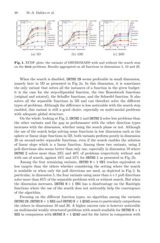
![ORTHOMADS on Continuous and Mixed-Integer Optimization Problems 39
ORTHO 2N. Besides, Neg reaches more targets on problems with low or moderate
conditioning. For these reasons, ORTHO N + 1 NEG was chosen for comparison with
other solvers. Besides, the mentioned slight advantage of ORTHO N + 1 QUAD over
ORTHO 2N, its equivalent or better performance on separable and ill-conditioned
functions compared with the latter variant, makes it a good second choice to
represent ORTHOMADS.
(a) 5D (b) 10D (c) 20D
Fig. 2. ECDF plots: the variants of ORTHOMADS with and without the search step
on the bbob-mixint problems. Results aggregated on all functions in dimensions 5, 10
and 20.
4 Comparison of ORTHOMADS with other solvers
The previous experiments showed the advantage of using the search step in
ORTHOMADS to speed up convergence. They also revealed the effectiveness of
some variants that are used here for comparisons with other algorithms on the
continuous and mixed-integer suites.
4.1 Compared Algorithms
Apart from ORTHOMADS, the other algorithms used for comparison on bbob
are first, three deterministic algorithms: the quasi-Newton Broyden-Fletcher-
Goldfarb-Shanno (BFGS) method [22], the quadratic model-based NEWUOA
and the adaptive N-M [14] that is a simplicial search. Stochastic methods are also
used among which a Random Search (RS) algorithm [10] and three population-
based algorithms: a surrogate-assisted CMA-ES, Differential Evolution (DE) [27]
and Particle Swarm Optimization (PSO) [11,18].
In order to perform algorithm comparisons on bbob-mixint, data from four
stochastic methods were collected: RS, the mixed-integer variant of CMA-ES,
DE and the Tree-structured Parzen Estimator (TPE) [8] that is a stochastic
model-based technique.
BFGS is an iterative quasi-Newton linesearch method that uses approxima-
tions of the Hessian matrix of the objective. At iteration k, the search direc-
tion pk solves a linear system Bkpk = −∇f(xk), where xk is the iterate, f the](https://image.slidesharecdn.com/optimizationlearningalgorithmsandapplications-231204021346-9e8015c0/85/Optimization-Learning-Algorithms-and-Applications-pdf-52-320.jpg)
![40 M.-A. Dahito et al.
objective function and Bk ≈ ∇2
f(xk). The matrix Bk is then updated according
to a formula. In the context of BBO, the derivatives are approximated with finite
differences.
NEWUOA is the Powell’s model-based algorithm for DFO. It is a trust-region
method that uses sequential quadratic interpolation models to solve uncon-
strained derivative-free problems.
The N-M method is a heuristic DFO method that uses simplices. It begins
with a non degenerated simplex. The algorithm identifies the worst point among
the vertices of the simplex and tries to replace it by reflection, expansion or
contraction. If none of these geometric transformations of the worst point enables
to find a better point, a contraction preserving the best point is done. The
adaptive N-M method uses the N-M technique with adaptation of parameters
to the dimension, which is notably useful in high dimensions.
RS is a stochastic iterative method that performs a random selection of
candidates: at each iteration, a random point is sampled and the best between
this trial point and the incumbent is kept.
CMA-ES is a state-of-the art evolutionary algorithm used in DFO. Let
N(m, C) denote a normal distribution of mean m and covariance matrix C.
It can be represented by the ellipsoid x
C−1
x = 1. The main axes of the ellip-
soid are the eigenvectors of C and the square roots of their lengths correspond
to the associated eigenvalues. CMA-ES iteratively samples its populations from
multivariate normal distributions. The method uses updates of the covariance
matrices to learn a quadratic model of the objective.
DE is a meta-heuristic that creates a trial vector by combining the incumbent
with randomly chosen individuals from a population. The trial vector is then
sequentially filled with parameters from itself or the incumbent. Finally the best
vector between the incumbent and the created vector is chosen.
PSO is an archive-based evolutionary algorithm where candidate solutions
are called particles and the population is a swarm. The particles evolve according
to the global best solution encountered but also according to their local best
points.
TPE is an iterative model-based method for hyperparameter optimization.
It sequentially builds a probabilistic model from already evaluated hyperparam-
eters sets in order to suggest a new set of hyperparameters to evaluate on a score
function that is to be minimized.
4.2 Parameter Setting
To compare the considered best variants of ORTHOMADS with other methods,
the 15 instances of each function were used and the maximal function evaluation
budget was increased to 105
× n, with n being the dimension.
For the bbob problems, the data used for BFGS, DE and the adaptive N-M
method comes from the experiments of [31]. CMA-ES was tested in [15], the
data of NEWUOA is from [26], the one of PSO is from [12] and RS results
come from [9]. The comparison data of CMA-ES, DE, RS and TPE used on](https://image.slidesharecdn.com/optimizationlearningalgorithmsandapplications-231204021346-9e8015c0/85/Optimization-Learning-Algorithms-and-Applications-pdf-53-320.jpg)
![ORTHOMADS on Continuous and Mixed-Integer Optimization Problems 41
the bbob-mixint suite comes from the experiments of [29]. All are accessi-
ble from the data archives of COCO with the cocopp.archives.bbob and
cocopp.archives.bbob mixint methods.
4.3 Results
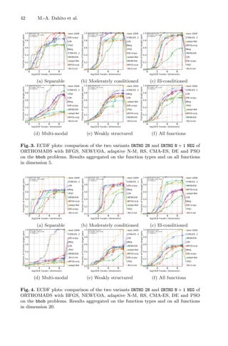
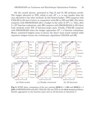
Continuous Problems. Figures 3 and 4 show the ECDF plots comparing the
methods on the different function types and on all functions, respectively in
dimensions 5 and 20 on the continuous suite. Compared with BFGS, CMA-ES,
DE, the adaptive N-M method, NEWUOA, PSO and RS, ORTHOMADS often
performs in the average for medium and high dimensions. For small dimensions
2 and 3, it is however among the most competitive.
Considering the results aggregated on all functions and splitting them over all
targets according to the function evaluations, they can be divided in three parts.
The first one consists of very limited budgets (about 20 × n) where NEWUOA
competes with or outperforms the others. After that, BFGS becomes the best
for an average budget and CMA-ES outperforms the latter for high evaluation
budgets (above the order of 102
× n), as shown in Figs. 3f and 4f. The obtained
performance restricted to a low budget is an important feature relevant to many
applications for which each function evaluation may last hours or even days.
On multi-modal problems with adequate structure, there is a noticeable gap
between the performance of CMA-ES, which is the best algorithm on this kind of
problems, and the other algorithms as shown by Figs. 3d and 4d. ORTHOMADS
performs the best in the remaining methods and competes with CMA-ES for
low budgets. It is even the best method up to a budget of 103
× n in 2D and 3D
while it competes with CMA-ES in higher dimensions for budgets lower than
the order of 102
× n.
RS is often the worse algorithm to use on the considered problems.
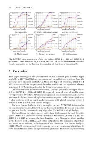
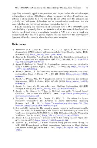
Mixed-Integer Problems. Figures 5 and 6 show the ECDF plots comparing
the methods on the different function types and on all functions, respectively
in dimensions 5 and 20 on the mixed-integer suite. The comparisons of NEG
and QUAD with CMA-ES, DE, RS and TPE show an overall advantage of these
ORTHOMADS variants over the other methods. A gap is especially visible on
separable and ill-conditioned problems, respectively depicted in Figs. 5a and 6a
and Figs. 5c and 6c in dimensions 5 and 20, but also on moderately conditioned
problems as shown in Figs. 5b and 6b in 5D and 20D. On multi-modal prob-
lems with global structure, ORTHOMADS is to prefer only in small dimensions:
from 10D its performance highly deteriorates and CMA-ES and DE seem to be
better choices. On multi-modal weakly structured functions, the advantages of
ORTHOMADS compared to the others emerge when the dimension increases.
Besides, although the performance of all algorithms decreases with increasing
dimensions, ORTHOMADS seems less sensitive to that. For instance, for a budget
of 102
× n, ORTHOMADS reaches 15% more targets than CMA-ES and TPE
that are the second best algorithms until this budget, and in dimension 20 this
gap increases to 18% for CMA-ES and 25% for TPE.](https://image.slidesharecdn.com/optimizationlearningalgorithmsandapplications-231204021346-9e8015c0/85/Optimization-Learning-Algorithms-and-Applications-pdf-54-320.jpg)

![A Look-Ahead Based Meta-heuristics
for Optimizing Continuous Optimization
Problems
Thomas Nordli and Noureddine Bouhmala(B)
University of South-Eastern Norway, Kongsberg, Norway
{thomas.nordli,noureddine.bouhmala}@usn.no
http://www.usn.no
Abstract. In this paper, the famous kernighan-Lin algorithm is adjusted
and embedded into the simulated annealing algorithm and the genetic
algorithm for continuous optimization problems. The performance of the
different algorithms are evaluated using a set of well known optimization
test functions.
Keywords: Continuous optimization problems · Simulated annealing ·
Genetic algorithm · Local search
1 Introduction
Several types of meta-heuristics methods have been designed for solving contin-
uous optimization problems. Examples include genetic algorithms [8,9] artificial
immune systems [7], and taboo search [5]. Meta-heuristics can be divided into
two different classes. The first class refers to single-solution search algorithms.
A notable example that belongs to this class is the popular simulated annealing
algorithm (SA) [12], which is a random search that avoids getting stuck in local
minima. In addition to solutions corresponding to an improvement in objective
function value, SA also accepts those corresponding to a worse objective function
value using a probabilistic acceptance strategy.
The second class of algorithms refer to population based algorithms. Algo-
rithms of this class applies the principle of survival of the fittest to a population
of potential solutions, iteratively improving the population. During each genera-
tion, pairs of solutions called individuals are generated to breed a new generation
using operators borrowed from natural genetics. This process is repeated until a
stopping criteria has been reached. Genetic algorithm is one among many that
belongs to this class. The following papers [1,2,6] provide a review of the lit-
erature covering the use of evolutionary algorithms for solving continuous opti-
mization problems. In spite of the advantages that meta-heuristics offer, they
still suffer from the phenomenon of premature convergence.
c
Springer Nature Switzerland AG 2021
A. I. Pereira et al. (Eds.): OL2A 2021, CCIS 1488, pp. 48–55, 2021.
https://doi.org/10.1007/978-3-030-91885-9_4](https://image.slidesharecdn.com/optimizationlearningalgorithmsandapplications-231204021346-9e8015c0/85/Optimization-Learning-Algorithms-and-Applications-pdf-61-320.jpg)
![A Look-Ahead Based Meta-heuristics for Continuous Optimization 49
Recently, several studies combined meta-heuristics with local search meth-
ods, resulting in more efficient methods with relatively faster convergence, com-
pared to pure meta-heuristics. Such hybrid approaches offer a balance between
diversification—to cover more regions of a search space, and intensification – to
find better solutions within those regions. The reader might refer to [3,14] for
further reading on hybrid optimization methods.
This paper introduces a hybridization of genetic algorithm and simulated
annealing with the variable depth search (VDS) Kernighan-Lin algorithm (KL)
(which was firstly presented for graph partitioning problem in [11]). Compared
to simple local search methods, KL allows making steps that worsens the quality
of the solution on a short term, as long as the result gives an improvement in a
longer run.
In this work, the search for one favorable move in SA, and one two-point
cross-over in GA, are replaced by a search for a favorable sequence of moves in
SA and a series of two-point crossovers using the objective function to guide
the search.
The rest of this paper is organized as follows. Section 2 describes the com-
bined simulated annealing and KL heuristic, while Sect. 3 explains the hybridiza-
tion of KL with the genetic algorithm. Section 4 lists the functions used in the
benchmark while Section 5 shows the experimental results. Finally, Sect. 6 con-
cludes the paper with some future work.
2 Combining Simulated Annealing with Local Search
Previously, SA in combination with KL, was applied for the Max-SAT problem in
[4]. SA iteratively improves a solution by making random perturbations (moves)
to the current solution—exploring the neighborhood in the space of possible
solutions. It uses a parameter called temperature to control the decision whether
to accept bad moves or not. A bad move is a solution that decreases the value
of the objective function.
The algorithm starts of with a high temperature, when that almost all
moves are accepted. For each iteration, the temperature decreases, the algorithm
becomes selective, giving higher preference for better solutions.
Assuming an objective function f is to be maximized. The algorithm starts
computing the initial temperature T, using a procedure similar to the one
described in [12]. The temperature is computed such that the probability of
accepting a bad move is approximately equal to a given probability of acceptance
Pr. First, a low value of is chosen as the initial temperature. This temperature
is used during a number of moves.
If the ratio of accepted bad moves is less than Pr, the temperature is multi-
plied by two. This continues until the observed acceptance ratio exceeds Pr. A
random starting solution is generated and its value is calculated. An iteration
of the algorithm starts by performing a series of so-called KL perturbations or
moves to the solution Sold leading to a new solution Si
new where i denotes the
number of consecutive moves. The change in the objective function called gain is](https://image.slidesharecdn.com/optimizationlearningalgorithmsandapplications-231204021346-9e8015c0/85/Optimization-Learning-Algorithms-and-Applications-pdf-62-320.jpg)
![50 T. Nordli and N. Bouhmala
computed for each move. The goal of KL perturbation is to generate a sequence
of objective function scores together with their corresponding moves. KL is sup-
posed to reach convergence if the function scores of five consecutive moves are
bad moves. The subset of moves having the best cumulative score BCSk
(SA+KL)
is identified. The identification of this subset is equivalent to choosing k so that
BCSk
(SA+KL) in Eq. 1 is maximum,
BCSk
(SA+KL) =
k
i=1
gain(Si
new) (1)
where i represents the ith
move performed, k the number of a moves, and
gain(Si
new) = f(Si
new) − f(Si−1
new) denotes the resultant change of the objective
function when ith
move has been performed. If BCSk
(SA+KL) 0, the solution
is updated by taking all the perturbations up to the index k and the best solu-
tion is always recorded. If (BCSk
SA+KL ≤ 0), the simulated acceptance test is
restricted to only the resultant change of the first perturbation. A number from
the interval (0,1) is drawn by a random number generator. The move is accepted
ff the drawn number is less than exp−δf/T
. The process of proposing a series of
perturbations and selecting the best subset of moves is repeated for a number of
iterations before the temperature is updated. A temperature reduction function
is used to lower the temperature. The updating of the temperature is done using
a geometric cooling, as shown in Eq. 2
Tnew = α × Told, where α = 0.9. (2)
3 Combining Genetic Algorithm with Local Search
Genetic Algorithm (GA) belong to the group of evolutionary algorithms. It works
on a set of solutions called a population. Each of these members, called chro-
mosomes or individuals, is given a score (fitness), allowing the assessing of its
quality. The individuals of the initial population are in most cases generated
randomly. A reproduction operator selects individuals as parents, and generates
off-springs by combining information from the parent chromosomes. The new
population might be subject to a mutation operator introducing diversity to the
population. A selection scheme is then used to update the population—resulting
in a new generation. This is repeated until the convergence is reached—giving
an optimal or near optimal solution.
The simple GA as described in [8] is used here. It starts by generating an ini-
tial population represented by floating point numbers. Solutions are temporary
converted to integers when bit manipulation is needed, and resulting integers are
converted back to floating point representation for storage. A roulette function
is used for selections. The implementation and based on the one described in
section IV of [10], where more details can be found.
The purpose of KL-Crossover is to perform the crossover operator a number
of times generating a sequence of fitness function scores together with their cor-
responding crossover. Thereafter, the subset of consecutive crossovers having the](https://image.slidesharecdn.com/optimizationlearningalgorithmsandapplications-231204021346-9e8015c0/85/Optimization-Learning-Algorithms-and-Applications-pdf-63-320.jpg)
![A Look-Ahead Based Meta-heuristics for Continuous Optimization 51
best cumulative score BCSk
(GA−KL) is determined. The identification of this sub-
set is the same as described in SA-KL. GA-KL chooses k so that BCSk
(GA+KL)
in Eq. 4 is maximum, where CRi
represents the ith
crossover performed on two
individuals, Il and Im, k the number of allowed crossovers, and gain(Il, Im)CRi
denotes the resulting change in the fitness function when the ith
crossover CRi
has been performed calculated shown in Eq. 3.
gain(Il, Im)CRi = f(Il, Im)CRi − f(Il, Im)CRi−1 , (3)
where CR0
refers to the chosen pair of parents before applying the cross-
over operator. KL-crossover is supposed to reach convergence if the gain of five
consecutive cross-overs is negative. Finally, the individuals that are best fit are
allowed to move to the next generation while the other half is removed and a
new round is performed.
BCSk
(GA+KL) = Max
k
i=1
gain(Individuall, Individualm)CRi
. (4)
4 Benchmark Functions and Parameter Setting
The stopping criterion for all four algorithms (SA, SA-Look-Ahead, GA, GA-
Look-Ahead) is supposed to be reached if the best solution has not been improved
during 100 consecutive iterations for (SA, SA-Look-Ahead) or 10 generations for
(GA, GA-Look-Ahead). The starting temperature for (SA, Look-Ahead-SA) is
set to 0.8 (i.e., a bad move has a probability of 80% for being accepted). In the
inner loop of (SA, Look-Ahead-SA), the equilibrium is reached if the number of
accepted moves is less than 10%.
The ten following benchmark functions were retrieved from [13] and tested.
1: Drop Wave f(x, y) = −
1+cos(12
x2+y2)
1
2
(x2+y2)+2
2: Griewangk f(x) = 1
4000
n
i=1 −
n
i=1 cos(
xi
√
i
) + 1
3: Levy Function sin2(3πx) + (x − 1)2[1 + sin2(3πy)] + (y − 1)2[1 + sin2(2πy)]
4: Rastrigin f(x) = 10n +
n
i=1(x2
i − 10 cos 2πxi)
5: Sphere Function f(x) =
n
i=1 x2
i
6: Weighted Sphere Function f(x, y) = x2 + 2y2
7: Sum of different power functions f(x) =
n
i=1 |xi|i+1
8: Rotated hyper-ellipsoid f(x) =
n
i=1
i
j=1 x2
j
9: Rosenbrock’s valley f(x) =
n−1
i=1
[100(xi+1 − x2
i )2 + (1 − xi)2]
10: Three Hump Camel Function f(x, y) = x2 − 1.05x4 + x6
6
+ xy + y2](https://image.slidesharecdn.com/optimizationlearningalgorithmsandapplications-231204021346-9e8015c0/85/Optimization-Learning-Algorithms-and-Applications-pdf-64-320.jpg)

![Inverse Optimization for Warehouse Management 57
the more complex an optimization model is needed, which can make it very
challenging to find a satisfactory solution in reasonable time, whether by generic
optimization algorithms or case-specific customized heuristics. Moreover, the
dynamic nature of business often necessitates regular updates to any decision
support tools as business processes and objectives change.
To make it easier to develop industrial decision support tools, one potential
approach is to apply machine learning methods to data from existing planning
processes. The data on actual decisions can be assumed to indicate the pref-
erences of competent decision makers, who have considered the effects of all
relevant factors and operational constraints in each decision. If a general control
policy can be derived from example decisions, the policy can then be replicated
in an automated decision support tool to reduce the manual planning effort,
or even completely automate the planning process. There would be no need to
explicitly model the preferences of the operational management at a particular
company. Ideally the control policy learned from data is generalisable to new
planning situations that differ from the training data, and can also be explained
in an understandable manner to business managers. In addition to implement-
ing tools for operational management, machine learning of management policies
could also be a useful tool when developing business simulation models for strate-
gic decision support.
The goal of this case study was to investigate whether inverse optimization
would be a suitable machine learning method to automate warehouse manage-
ment on the basis of demonstration data. In the study, inverse optimization
was applied to the problem of storage location assignment, i.e. where to place
incoming packages in a large warehouse. A mixed-integer model and a column
generation procedure were formulated for dynamic class-based storage location
assignment, with explicit consideration for the arrival and departure points of
goods, and possible congestion in warehouse stocking and picking activities.
The main contributions of the study are 1) combining the inverse optimiza-
tion approach of Ahuja and Orlin [1] with a cutting plane algorithm in the
first known application of inverse optimization to a storage location assignment
problem, and 2) computational experiments on applying the estimated objective
function in a practical rolling horizon procedure with real-world data.
2 Related Work
A large variety of analytical approaches have been published for warehouse
design and management [6,8,12,21]. Hausman et al. [10] presented an early
analysis of basic storage location assignment methods including random stor-
age, turnover-based storage in which highest-turnover products are assigned to
locations with the shortest transport distance, and class-based storage in which
products are grouped into classes that are associated with areas of the warehouse.
The location allocation decisions of class-based storage policies may be based on
simple rules such as turnover-based ordering, or an explicit optimization model
as in [18].](https://image.slidesharecdn.com/optimizationlearningalgorithmsandapplications-231204021346-9e8015c0/85/Optimization-Learning-Algorithms-and-Applications-pdf-70-320.jpg)
![58 H. Rummukainen
Goetschalckx and Ratliff [7] showed that information about storage durations
of arriving units can be used in a duration-of-stay-based (DOS-based) shared
storage policy that is more efficient than an optimal static dedicated (class-
based or product-based) storage policy. Kim and Park [13] used a subgradient
optimization algorithm for location allocation, assuming full knowledge of stor-
age times and amounts over the planning interval. Chen et al. [5] presented a
mixed-integer model and heuristic algorithms to minimize the peak transport
load of a DOS-based policy. In the present study, more complex DOS-based
policies are considered, with both dynamic class-based location assignment and
congestion costs.
Updating class-based assignments regularly was proposed by Pierre et al. [20],
and further studied by Kofler et al. [14], who called the problem multi-period
storage location assignment. Their problem was quite similar to the present
study, but both Pierre et al. and Kofler et al. applied heuristic rules without an
explicit mathematical programming model, and also included reshuffling moves.
The problem of yard planning in container terminals is closely related to
warehouse management, and a number of detailed optimization models have
been published. [17,24] Congestion constraints for lanes in the yard were already
considered by Lee et al. [9,15] Moccia et al. [16] considered storage location
assignment as a dynamic generalized assignment problem, in which goods could
be relocated over time, but each batch of goods would have to be treated as an
unsplittable unit. The present study does not address relocation, but is differ-
entiated by class-based assignment, as well as the use of inverse optimization.
Pang and Chan [19] applied a data mining algorithm as a component of
a dynamic storage location assignment algorithm, but they did not use any
external demonstration policy in their approach.
Learning to replicate a control policy demonstrated by an expert has been
studied by several computational methods, in particular as inverse optimiza-
tion [1,3,22] and inverse reinforcement learning [2]. Compared to more generic
supervised machine learning methods, inverse optimization and reinforcement
learning methods have the advantage that they can take into account the future
consequences of present-time actions. The author is not aware of any prior work
in applying inverse optimization or inverse reinforcement learning to warehouse
management problems.
In a rolling horizon procedure, the plan is reoptimized regularly so that con-
secutive planning periods overlap. Troutt et al. [23] considered the problem of
estimating the objective function of a rolling horizon optimization procedure
from demonstrated decisions. They assumed that the initial state for each plan-
ning period could be fixed according to the demonstrated decisions, and then
minimized the sum of decisional regret over the planning periods: the decisional
regret of a planning period was defined as a function of objective function coeffi-
cients, and equals the gap between the optimal objective value and the objective
value of the demonstrated decisions over the planning period. In the present
study, the inverse optimization was performed on a model covering the full](https://image.slidesharecdn.com/optimizationlearningalgorithmsandapplications-231204021346-9e8015c0/85/Optimization-Learning-Algorithms-and-Applications-pdf-71-320.jpg)
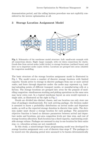
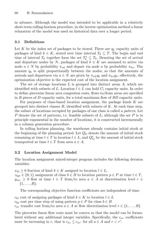
![Inverse Optimization for Warehouse Management 63
Potentially profitable patterns can be found by detecting violations of dual
constraint (13). Specifically, the procedure seeks p ⊆ L, b ∈ B and t ∈ T that
maximize, and reach a positive value for the expression
ψbt −
l∈p
φtl +
k∈b: Tkt,
l∈p
ξktl − cbp = ψbt −
l∈p
(φtl + γl −
k∈b: Tkt
ξktl) − δ max
l,l∈p
d0
ll ,
where the definition (9) of cbp has been expanded. Let us denote by Vlbt the
parenthesized expression on the right-hand side, and by qbt =
k∈b: Tkt qk the
amount of class b goods at time t. The column generation subproblem for given b
and t is defined in terms of the following decision variables: ul ∈ {0, 1} indicates
whether location l ∈ L belongs in the pattern, vlk ≥ 0 indicates ordered pairs
of locations l, k ∈ L that both belong in the pattern, and s ≥ 0 represents
the diameter of the pattern. The subproblem is formulated as a mixed-integer
program:
min
l∈L
Vlbtul + δs (16)
l∈L
CMl ul ≥ qbt (17)
s − d0
lkvlk ≥ 0 ∀l, k ∈ L, l k (18)
vlk − ul − uk ≥ −1 ∀l, k ∈ L, l k (19)
The constraint (17) ensures that the selected locations together have sufficient
capacity to be feasible in the location assignment problem. The constraints (18)
bound s to match the pattern diameter, and (19) together with the minimization
objective ensure that vlk = uluk for all l, k ∈ L.
In the column generation procedure, the problem (16)–(19) is solved itera-
tively by a mixed-integer solver for all classes b ∈ B and time steps t ∈ T, and
whenever the objective is smaller than ψbt, the pattern defined by the corre-
sponding solution is added to the set of patterns P. After all b and t have been
checked, the linear program (1)–(8) is resolved with the updated P, and the
column generation procedure is repeated with newly obtained values of (ψ, φ, ξ).
If no more profitable patterns are found or the algorithm runs out of time, the
current patterns P are fixed and finally the location assignment problem (1)–(8)
is resolved as a mixed-integer program.
Note that cbp is a submodular function of p. Kamiyama [11] presented a
polynomial-time approximation algorithm for minimizing a submodular function
with covering-type constraints (which (17) is), but in this study it was considered
simpler to use a mixed-integer solver.
4 Inverse Optimization Method
The location assignment decisions demonstrated by the human decision makers
are assumed to form a feasible solution (z, x, y) to the location assignment model](https://image.slidesharecdn.com/optimizationlearningalgorithmsandapplications-231204021346-9e8015c0/85/Optimization-Learning-Algorithms-and-Applications-pdf-76-320.jpg)
![64 H. Rummukainen
(1)–(8). The goal of the presented inverse optimization method is to estimate
the parameters of the cost model in the form (9)–(11), so that the demonstrated
solution (z, x, y) is optimal or near-optimal for the costs c.
The demonstrated solution is not assured to be an extreme point, and may
be in the relative interior of the feasible region. Moreover, with costs restricted
to the form (9)–(11), non-trivial (unique) optimality may be impossible for even
some boundary points of the primal feasible region. Because of these issues, in
contrast with the inverse linear optimization method of Ahuja and Orlin [1],
complementary slackness conditions are not fully enforced, and the duality gap
between the primal (1) and dual (12) objectives is minimized as an objective.
To make sure that the inverse problem is feasible with nontrivial c, none of
the dual constraints (13)–(15) is tightened to strict equality by complementary
slackness. Nevertheless, the following additional constraints on the dual solution
(ψ, φ, ξ, μ, λ, η, θ) are enforced on the basis of complementary slackness with the
fixed primal solution (z, x, y):
φtl = 0 ∀t ∈ T, l ∈ L :
b∈B, pl zbpt 1 (20)
ξktl = 0 ∀b ∈ B, k ∈ b, t ∈ T, l ∈ L : xkl −
pl zbpt 0 (21)
λtlm = 0 ∀t ∈ T, l ∈ L, m = 1, . . . , Ml : wtlm C (22)
θtar = 0 ∀t ∈ T, a ∈ A, , r = 1, . . . , R : ytar D (23)
The duality gap that is to be minimized is given by
Γ =
b∈B, p∈P,
t∈T
cbpzbpt +
k∈K, l∈L
cklxkl +
t∈T, l∈L,
m=1,...,Ml
clmwtlm +
t∈T, a∈A,
r=1,...,R
carytar
−
b∈B, t∈T
ψbt +
t∈T, l∈L
φtl −
k∈K
μk +
t∈T, l∈L
(Cl − Qtl)λtl −
t∈T, a∈A
Q
taηta +
t∈T, a∈A,
r=1,...,R
Dθtar. (24)
Note that Γ ≥ 0 because (z, x, y) is primal feasible and (ψ, φ, ξ, μ, λ, η, θ) is dual
feasible.
Similarly to Ahuja and Orlin [1], the cost estimation is regularized by penalis-
ing deviations from nominal cost values, but in a more specific formulation. The
deviation objective term is defined as follows, weighting cost model parameters
approximately in proportion to their contribution to the primal objective:
Δ =
t∈T
b∈B
k∈b: Tkt qk
l∈L CMl
l∈L
γl − γ0
l
+
maxl,l∈L d0
ll
2
δ − δ0
+
k∈K
qk
|L|
l∈L
n∈N
πnk
dnl − d0
nl
+ πkn
dln − d0
ln
+
k∈K
2qk
R
r=1
r
j=1
αj − α0
j
(25)
As this is a minimization objective, the standard transformation of absolute
value terms to linear programming constraints and variables applies [4, p. 17].](https://image.slidesharecdn.com/optimizationlearningalgorithmsandapplications-231204021346-9e8015c0/85/Optimization-Learning-Algorithms-and-Applications-pdf-77-320.jpg)
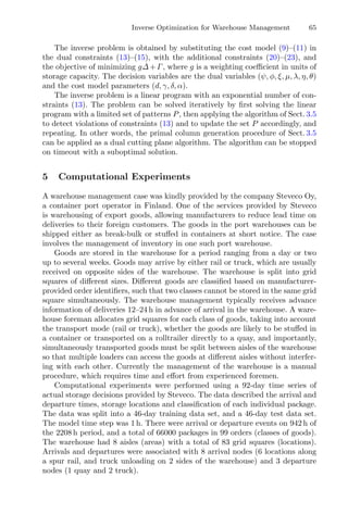
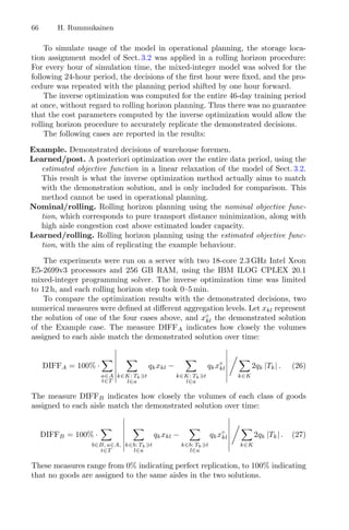
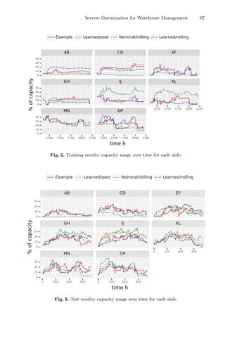
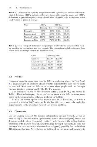
![Inverse Optimization for Warehouse Management 69
Table 1, the results of the rolling horizon procedure were closer to the demon-
strated decisions after the inverse optimization (Learned/rolling) than before
(Nominal/rolling).
On the test data set, as seen in Fig. 3 and Table 1, the continuous optimiza-
tion results (Learned/post) diverged further from the demonstrated decisions
(Example) than in the training data set. The results of the rolling horizon pro-
cedure however appeared to follow the demonstrated decisions somewhat better
than on the training data set, both visually and by the DIFFA measure. Again,
the results of the rolling horizon procedure were closer to the demonstrated
decisisions after the inverse optimization (Learned/rolling) than before (Nomi-
nal/rolling).
Replicating the demonstrated decisions in more detail than at the level of per-
aisle capacity usage was unsuccessful so far. As shown by the DIFFB measure
in Table 1, classes of goods were largely assigned to different aisles than in the
demonstrated decisions. A particular difficulty in the case study was that there
was no machine-readable data on the properties of the classes beyond an opaque
order identifier.
Besides the difficulties at the level of classes of goods, comparing the assign-
ments at the level of individual locations was also fruitless. The preliminary
conclusion was that since most of the goods would flow through the warehouse
aisles from one side to another, choosing one grid square or another in the same
aisle would not make a substantial difference in the total work required.
Although matching the demonstrated decisions by inverse optimization had
limited success so far, the storage location assignment model of Sect. 3 was found
to be valuable. In the Nominal/rolling case, in which the objective was to mini-
mize transport distances with congestion penalties, the total transport distance
of the packages was reduced by 13–15% compared to manual planning, as can
be seen in Table 2. Based on the computational experiments, the model has the
potential to be useful for warehouse management on realistic scale.
While the algorithm appeared to converge in 12 h with the 46-day training
data set, this was at the limit of the current capabilities of the method. In
an abandoned attempt to use a 50% larger training data set, the algorithm
progressed over 10 times slower than in the presented runs. In particular the size
of the location assignment model is sensitive to the size of the set K, i.e. the
number of kinds of packages.
6 Conclusion
The inverse optimization approach of Ahuja and Orlin [1] was applied to the
linear relaxation of a mixed-integer storage location assignment problem, and a
solution method based on a cutting plane algorithm was presented. The method
was tested on real-world data, and the estimated objective function was used in
the mixed-integer model in a practical short-term rolling-horizon procedure.
The inverse optimization method and the rolling-horizon procedure were able
to coarsely mimic a demonstrated storage location assignment policy on the](https://image.slidesharecdn.com/optimizationlearningalgorithmsandapplications-231204021346-9e8015c0/85/Optimization-Learning-Algorithms-and-Applications-pdf-82-320.jpg)
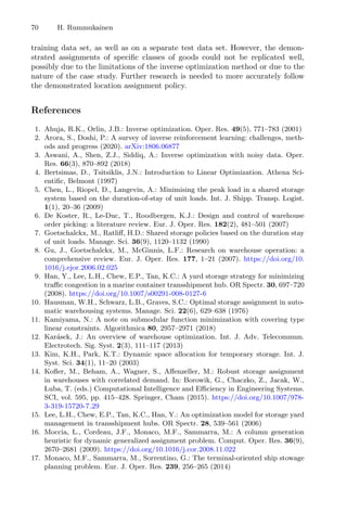

![Model-Agnostic Multi-objective
Approach for the Evolutionary Discovery
of Mathematical Models
Alexander Hvatov(B)
, Mikhail Maslyaev, Iana S. Polonskaya,
Mikhail Sarafanov, Mark Merezhnikov, and Nikolay O. Nikitin
NSS (Nature Systems Simulation) Lab, ITMO University,
Saint-Petersburg, Russia
{alex hvatov,mikemaslyaev,ispolonskaia,
mik sar,mark.merezhnikov,nnikitin}@itmo.ru
Abstract. In modern data science, it is often not enough to obtain only
a data-driven model with a good prediction quality. On the contrary, it is
more interesting to understand the properties of the model, which parts
could be replaced to obtain better results. Such questions are unified
under machine learning interpretability questions, which could be consid-
ered one of the area’s raising topics. In the paper, we use multi-objective
evolutionary optimization for composite data-driven model learning to
obtain the algorithm’s desired properties. It means that whereas one
of the apparent objectives is precision, the other could be chosen as
the complexity of the model, robustness, and many others. The method
application is shown on examples of multi-objective learning of compos-
ite models, differential equations, and closed-form algebraic expressions
are unified and form approach for model-agnostic learning of the inter-
pretable models.
Keywords: Model discovery · Multi-objective optimization ·
Composite models · Data-driven models
1 Introduction
The increasing precision of the machine learning models indicates that the best
precision model is either overfitted or very complex. Thus, it is used as a black
box without understanding the principle of the model’s work. This fact means
that we could not say if the model can be applied to another sample without
a direct experiment. Related questions such as applicability to the given class
of the problems, sensitivity, and the model parameters’ and hyperparameters’
meaning arise the interpretability problem [7].
In machine learning, two approaches to obtain the model that describes the
data are existing. The first is to fit the learning algorithm hyperparameters and
the parameters of a given model to obtain the minimum possible error. The
second one is to obtain the model structure (as an example, it is done in neural
c
Springer Nature Switzerland AG 2021
A. I. Pereira et al. (Eds.): OL2A 2021, CCIS 1488, pp. 72–85, 2021.
https://doi.org/10.1007/978-3-030-91885-9_6](https://image.slidesharecdn.com/optimizationlearningalgorithmsandapplications-231204021346-9e8015c0/85/Optimization-Learning-Algorithms-and-Applications-pdf-85-320.jpg)
![Multi-objective Discovery of Mathematical Models 73
architecture search [1]) or the sequence of models that describe the data with the
minimal possible error [12]. We refer to obtaining a set of models or a composite
model as a composite model discovery.
After the model is obtained, both approaches may require additional model
interpretation since the obtained model is still a black box. For model interpre-
tation, many different approaches exist. One group of approaches is the model
sensitivity analysis [13]. Sensitivity analysis allows mapping the input variability
to the output variability. Algorithms from the sensitivity analysis group usually
require multiple model runs. As a result, the model behavior is explained rela-
tively, meaning how the output changes with respect to the input changing.
The second group is the explaining surrogate models that usually have less
precision than the parent model but are less complex. For example, linear regres-
sion models are used to explain deep neural network models [14]. Additionally,
for convolutional neural networks that are often applied to the image classi-
fication/regression task, visual interpretation may be used [5]. However, this
approach cannot be generalized, and thus we do not put it into the classification
of explanation methods.
All approaches described above require another model to explain the results.
Multi-objective optimization may be used for obtaining a model with desired
properties that are defined by the objectives. The Pareto frontier obtained during
the optimization can explain how the objectives affect the resulting model’s
form. Therefore, both the “fitted” model and the model’s initial interpretation
are achieved.
We propose a model-agnostic data-driven modeling method that can be used
for an arbitrary composite model with directed acyclic graph (DAG) represen-
tation. We assume that the composite model graph’s vertices (or nodes) are the
models and the vertices define data flow to the final output node. Genetic pro-
gramming is the most general approach for the DAG generation using evolution-
ary operators. However, it cannot be applied to the composite model discovery
directly since the models tend to grow unexpectedly during the optimization
process.
The classical solution is to restrict the model length [2]. Nevertheless, the
model length restriction may not give the best result. Overall, an excessive
amount of models in the graph drastically increases the fitting time of a given
composite model. Moreover, genetic programming requires that the resulting
model is computed recursively, which is not always possible in the composite
model case.
We refine the usual for the genetic programming cross-over and mutation
operators to overcome the extensive growth and the model restrictions. Addition-
ally, a regularization operator is used to retain the compactness of the resulting
model graph. The evolutionary operators, in general, are defined independently
on a model type. However, objectives must be computed separately for every
type of model. The advantage of the approach is that it can obtain a data-
driven model of a given class. Moreover, the model class change does not require
significant changes in the algorithm.](https://image.slidesharecdn.com/optimizationlearningalgorithmsandapplications-231204021346-9e8015c0/85/Optimization-Learning-Algorithms-and-Applications-pdf-86-320.jpg)
![74 A. Hvatov et al.
We introduce several objectives to obtain additional control over the model
discovery. The multi-objective formulation allows giving an understanding of how
the objectives affect the resulting model. Also, the Pareto frontier provides a set
of models that an expert could assess and refine, which significantly reduces
time to obtain an expert solution when it is done “from scratch”. Moreover,
the multi-objective optimization leads to the overall quality increasing since the
population’s diversity naturally increases.
Whereas the multi-objective formulation [15] and genetic programming [8]
are used for the various types of model discovery separately, we combine both
approaches and use them to obtain a composite model for the comprehensive
class of atomic models. In contrast to the composite model, the atomic model
has single-vector input, single-vector output, and a single set of hyperparameters.
As an atomic model, we may consider a single model or a composite model that
undergoes the “atomization” procedure. Additionally, we consider the Pareto
frontier as the additional tool for the resulting model interpretability.
The paper is structured as follows: Sect. 2 describes the evolutionary oper-
ators and multi-objective optimization algorithms used throughout the paper,
Sect. 3 describes discovery done on the same real-world application dataset for
particular model classes and different objectives. In particular, Sect. 3.2 describes
the composite model discovery for a class of the machine learning models with
two different sets of objective functions; Sect. 3.3 describes the closed-form alge-
braic expression discovery; Sect. 3.4 describes the differential equation discovery.
Section 4 outlines the paper.
2 Problem Statement for Model-Agnostic Approach
The developed model agnostic approach could be applied to an arbitrary com-
posite model represented as a directed acyclic graph. We assume that the graph’s
vertices (or nodes) are the atomic models with parameters fitted to the given
data. It is also assumed that every model has input data and output data. The
edges (or connections) define which models participate in generating the given
model’s input data.
Before the direct approach description, we outline the scheme Fig. 1 that
illustrates the step-by-step questions that should be answered to obtain the
composite model discovery algorithm.
For our approach, we aim to make Step 1 as flexible as possible. Approach
application to different classes of functional blocks is shown in Sect. 3. The
realization of Step 2 is described below. Moreover, different classes of models
require different qualitative measures (Step 3), which is also shown in Sect. 3.
The cross-over and mutation schemes used in the described approach do not
differ in general from typical symbolic optimization schemes. However, in con-
trast to the usual genetic programming workflow, we have to add regularization
operators to restrict the model growth. Moreover, the regularization operator
allows to control the model discovery and obtain the models with specific prop-
erties. In this section, we describe the generalized concepts. However, we note](https://image.slidesharecdn.com/optimizationlearningalgorithmsandapplications-231204021346-9e8015c0/85/Optimization-Learning-Algorithms-and-Applications-pdf-87-320.jpg)
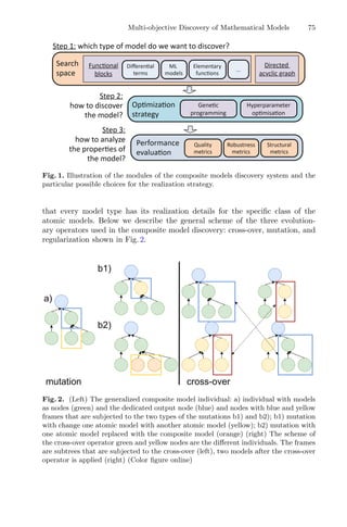
![76 A. Hvatov et al.
The mutation operator has two variations: node replacement with another
node and node replacement with a sub-tree. Scheme for the both type of the
mutations are shown in Fig. 2(left). The two types of mutation can be applied
simultaneously. The probabilities of the appearance of a given type of mutation
are the algorithm’s hyperparameters. We note that for convenience, some nodes
and model types may be “immutable”. This trick is used, for example, in Sect.3.4
to preserve the differential operator form and thus reduce the optimization space
(and consequently the optimization time) without losing generality.
In general, the cross-over operator could be represented as the subgraphs
exchange between two models as shown in Fig. 2(right). In the most general case,
in the genetic programming case, subgraphs are chosen arbitrarily. However,
since not all models have the same input and output, the subgraphs are chosen
such that the inputs and outputs of the offspring models are valid for all atomic
models.
In order to restrict the excessive growth of the model, we introduce an addi-
tional regularization operator shown in Fig. 3. The amount of described disper-
sion (as an example, using the R2 metric) is assessed for each graph’s depth
level. The models below the threshold are removed from the tree iteratively with
metric recalculation after each removal. Also, the applied implementation of the
regularization operator can be task-specific (e.g., custom regularization for com-
posite machine learning models [11] and the LASSO regression for the partial
differential equations [9]).
Fig. 3. The scheme of the regularization operator. The numbers are the dispersion
ratio that is described by the child nodes as the given depth level. In the example
model with dispersion ratio 0.1 is removed from the left model to obtain simpler model
to the right.
Unlike the genetic operators defined in general, the objectives are defined for
the given class of the atomic models and the given problem. The class of the
models defines the way of an objective function computation. For example, we
consider the objective referred to as “quality”, i.e., the ability of the given com-
posite model to predict the data in the test part of the dataset. Machine learning
models may be additionally “fitted” to the data with a given composite model
structure. Fitting may be used for all models simultaneously or consequently
for every model. Also, the parameters of the machine learning models may not](https://image.slidesharecdn.com/optimizationlearningalgorithmsandapplications-231204021346-9e8015c0/85/Optimization-Learning-Algorithms-and-Applications-pdf-89-320.jpg)
![Multi-objective Discovery of Mathematical Models 77
be additionally optimized, which increases the optimization time. The differen-
tial equations and the algebraic expressions realization atomic models are more
straightforward than the machine learning models. The only way to change the
quality objective is the mutation, cross-over, and regularization operators. We
note that there also may be a “fitting” procedure for the differential equations.
However, we do not introduce variable parameters for the differential terms in
the current realization.
In the initial stage of the evolution, according to the standard workflow
of the MOEA/DD [6] algorithm, we have to evaluate the best possible value
for each of the objective functions. The selection of parents for the cross-over
is held for each objective function space region. With a specified probability
of maintaining the parents’ selection, we can select an individual outside the
processed subregion to partake in the recombination. In other cases, if there are
candidate solutions in the region associated with the weights vector, we make
a selection among them. The final element of MOEA/DD is population update
after creating new solutions, which is held without significant modifications. The
resulting algorithm is shown in Algorithm 1.
Data: Class of atomic models T = {T1, T2, ... Tn}; (optional) define subclass of
immutable models; objective functions
Result: Pareto frontier
Create a set of weight vectors w = (w1
, ..., wn weights
), wi
= (wi
1, ..., wi
n eq+1);
for weight vector in weights do
Select K nearest weight vectors to the weight vector;
Randomly generate a set of candidate models divide them into
non-dominated levels;
Divide the initial population into groups by subregion, to which they belong;
for epoch = 1 to epoch number do
for weight vector in weights do
Parent selection;
Apply recombination to parents pool and mutation to individuals inside
the region of weights (Fig. 2);
for offspring in new solutions do
Apply regularization operator (Fig. 3);
Get values of objective functions for offspring;
Update population;
Algorithm 1: The pseudo-code of model-agnostic Pareto frontier construction
To sum up, the proposed approach combines classical genetic programming
operators with the regularization operator and the immutability property of
selected nodes. The refined MOEA/DD and refined genetic programming oper-
ators obtain composite models for different atomic model classes.](https://image.slidesharecdn.com/optimizationlearningalgorithmsandapplications-231204021346-9e8015c0/85/Optimization-Learning-Algorithms-and-Applications-pdf-90-320.jpg)
![78 A. Hvatov et al.
3 Examples
In this section, several applications of the described approach are shown. We use
a common dataset for all experiments that are described in the Sect. 3.1.
While the main idea is to show the advantages of the multi-objective app-
roach, the particular experiments show different aspects of the approach realiza-
tion for different models’ classes. Namely, we want to show how different choices
of the objectives reflect the expert modeling.
For the machine learning models in Sect. 3.2, we try to mimic the expert’s
approach to the model choice that allows one to transfer models to a set of
related problems and use a robust regularization operator.
Almost the same idea is pursued in mathematical models. Algebraic expres-
sion models in Sect. 3.3 are discovered with the model complexity objective. More
complex models tend to reproduce particular dataset variability and thus may
not be generalized. To reduce the optimization space, we introduce immutable
nodes to restrict the model form without generality loss. The regularization oper-
ator is also changed to assess the dispersion relation between the model residuals
and data, which has a better agreement with the model class chosen.
While the main algebraic expressions flow is valid for partial differential equa-
tions discovery in Sect. 3.4, they have specialties, such as the impossibility to
solve intermediate models “on-fly”. Therefore LASSO regularization operator is
used.
3.1 Experimental Setup
The validation of the proposed approach was conducted for the same dataset
for all types of models: composite machine learning models, models based on
closed-form algebraic expression, and models in differential equations.
The multi-scale environmental process was selected as a benchmark. As the
dataset for the examples, we take the time series of sea surface height were
obtained from numerical simulation using the high-resolution setup of the NEMO
model for the Arctic ocean [3]. The simulation covers one year with the hourly
time resolution. The visualization of the experimental data is presented in Fig. 4.
It is seen from Fig. 4 that the dataset has several variability scales. The com-
posite models, due to their nature, can reproduce multiple scales of variability.
In the paper, the comparison between single and composite model performance
is taken out of the scope. We show only that with a single approach, one may
obtain composite models of different classes.
3.2 Composite Machine Learning Models
The machine learning pipelines’ discovery methods are usually referred to as
automated machine learning (AutoML). For the machine learning model design,
the promising task is to control the properties of obtained model. Quality and
robustness could be considered as an example of the model’s properties. The](https://image.slidesharecdn.com/optimizationlearningalgorithmsandapplications-231204021346-9e8015c0/85/Optimization-Learning-Algorithms-and-Applications-pdf-91-320.jpg)
![Multi-objective Discovery of Mathematical Models 79
Fig. 4. The multi-scale time series of sea surface height used as a dataset for all exper-
iments.
proposed model-agnostic approach can be used to discover the robust compos-
ite machine learning models with the structure described as a directed acyclic
graph (as described in [11]). In this case, the building blocks are regression-based
machine learning models, algorithms for feature selection, and feature transfor-
mation. The specialized lagged transformation is applied to the input data to
adapt the regression models for the time series forecasting. This transformation
is also represented as a building block for the composite graph [4].
The quality of the composite machine learning models can be analyzed in
different ways. The simplest way is to estimate the quality of the prediction on
the test sample directly. However, the uncertainty in both models and datasets
makes it necessary to apply the robust quality evaluation approaches for the
effective analysis of modeling quality [16].
The stochastic ensemble-based approach can be applied to obtain the set of
predictions Yens for different modeling scenarios using stochastic perturbation of
the input data for the model. In this case, the robust objective function
fi (Yens)
can be evaluated as follows:
μens = 1
k
k
j=1 (Y j
ens) + 1,
fi (Yens) = μens
1
k−1
k
i=1 (fi (Y i
ens) − μens)
2
+ 1
(1)
In Eq. 1 k is the number of models in the ensemble, f - function for modelling
error, Yens - ensemble of the modelling results for specific configuration of the
composite model.
The robust and non-robust error measures of the model cannot be minimized
together. In this case, the multi-objective method proposed in the paper can be
used to build the predictive model. We implement the described approach as a
part of the FEDOT framework1
that allow building various ML-based composite
models. The previous implementation of FEDOT allows us to use multi-objective
1
https://github.com/nccr-itmo/FEDOT.](https://image.slidesharecdn.com/optimizationlearningalgorithmsandapplications-231204021346-9e8015c0/85/Optimization-Learning-Algorithms-and-Applications-pdf-92-320.jpg)
![Multi-objective Discovery of Mathematical Models 81
a free parameters (as an example T = (t; α1, α2, α3) = α3 sin(α1t + α2) with
free parameters set α1, α2, α3), which are subject to optimization. In the present
paper, we use pulses, polynomials, and trigonometric functions as the tokens set.
For the mathematical expression models overall, it is helpful to introduce two
groups of objectives. The first group of the objectives we refer to as “quality”.
For a given equation M, the quality metric ||·|| is the data D reproduction norm
that is represented as
Q(M) = ||M − D|| (2)
The second group of objectives we refer to as “complexity”. For a given
equation M, the complexity metric is bound to the length of the equation that
is denoted as #(M)
C(M) = #(M) (3)
As an example of objectives, we use rooted mean squared error (RMSE) as
the quality metric and the number of tokens present in the resulting model as the
complexity metric. First, the model’s structure is obtained with a separate evo-
lutionary algorithm to compute the mean squared error. In details it is described
in [10].
To perform the single model evolutionary optimization in this case, we make
the arithmetic operations immutable. The resulting directed acyclic graph is
shown in Fig. 6. Thus, the third type of nodes appears - immutable ones. This
step is not necessary, and the general approach described above may be used
instead. However, it reduces the search space and thus reduces the optimization
time without losing generality.
Fig. 6. The scheme of the composite model, generalizing the discovered differential
equation, where red nodes are the nodes, unaffected by mutation or cross-over operators
of the evolutionary algorithm. The blue nodes represent the tokens that evolutionary
operators can alter. (Color figure online)
The resulting Pareto frontier for the class of the described class of closed-form
algebraic expressions is shown in Fig. 7.](https://image.slidesharecdn.com/optimizationlearningalgorithmsandapplications-231204021346-9e8015c0/85/Optimization-Learning-Algorithms-and-Applications-pdf-94-320.jpg)
![82 A. Hvatov et al.
Fig. 7. The Pareto frontier for the evolutionary multi-objective design of the closed-
form algebraic expressions. The root mean squared error (RMSE) and model complex-
ity are used as objective functions.
Since the origin of time series is the sea surface height in the ocean, it is
natural to expect that the closed-form algebraic expression is the spectra-like
decomposition, which is seen in Fig. 7. It is also seen that as soon as the com-
plexity rises, the additional term only adds information to the model without
significant changes to the terms that are present in the less complex model.
3.4 Differential Equations
The development of a differential equation-based model of a dynamic system can
be viewed from the composite model construction point of view. A tree graph rep-
resents the equation with input functions, decoded as leaves, and branches repre-
senting various mathematical operations between these functions. The specifics
of a single equation’s development process were discussed in the article [9].
The evaluation of equation-based model quality is done in a pattern similar to
one of the previously introduced composite models. Each equation represents a
trade-off between its complexity, which we estimate by the number of terms in it
and the quality of a process representation. Here, we will measure this process’s
representation quality by comparing the left and right parts of the equation.
Thus, the algorithm aims to obtain the Pareto frontier with the quality and
complexity taken as the objective functions.
We cannot use standard error measures such as RMSE since the partial
differential equation with the arbitrary operator cannot be solved automatically.
Therefore, the results from previous sections could not be compared using the
quality metric.](https://image.slidesharecdn.com/optimizationlearningalgorithmsandapplications-231204021346-9e8015c0/85/Optimization-Learning-Algorithms-and-Applications-pdf-95-320.jpg)
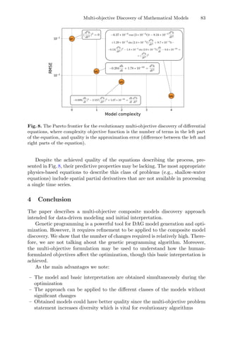
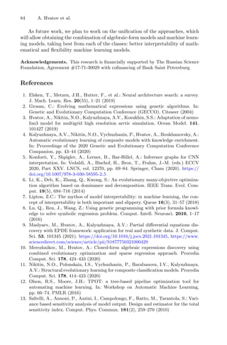

![A Simple Clustering Algorithm Based
on Weighted Expected Distances
Ana Maria A. C. Rocha1(B)
, M. Fernanda P. Costa2
,
and Edite M. G. P. Fernandes1
1
ALGORITMI Center, University of Minho, Campus de Gualtar,
4710-057 Braga, Portugal
{arocha,emgpf}@dps.uminho.pt
2
Centre of Mathematics, University of Minho, Campus de Gualtar,
4710-057 Braga, Portugal
mfc@math.uminho.pt
Abstract. This paper contains a proposal to assign points to clusters,
represented by their centers, based on weighted expected distances in a
cluster analysis context. The proposed clustering algorithm has mecha-
nisms to create new clusters, to merge two nearby clusters and remove
very small clusters, and to identify points ‘noise’ when they are beyond
a reasonable neighborhood of a center or belong to a cluster with very
few points. The presented clustering algorithm is evaluated using four
randomly generated and two well-known data sets. The obtained cluster-
ing is compared to other clustering algorithms through the visualization
of the clustering, the value of the DB validity measure and the value
of the sum of within-cluster distances. The preliminary comparison of
results shows that the proposed clustering algorithm is very efficient and
effective.
Keywords: Clustering analysis · Partitioning algorithms · Weighted
distance
1 Introduction
Clustering is an unsupervised machine learning task that is considered one of
the most important data analysis techniques in data mining. In a clustering
problem, unlabeled data objects are to be partitioned into a certain number of
groups (also called clusters) based on their attribute values. The objective is that
objects in a cluster are more similar to each other than to objects in another
cluster [1–4]. In geometrical terms, the objects can be viewed as points in a
a-dimensional space, where a is the number of attributes. Clustering partitions
these points into groups, where points in a group are located near one another
in space.
This work has been supported by FCT – Fundação para a Ciência e Tecnologia within
the RD Unit Project Scope UIDB/00319/2020.
c
Springer Nature Switzerland AG 2021
A. I. Pereira et al. (Eds.): OL2A 2021, CCIS 1488, pp. 86–101, 2021.
https://doi.org/10.1007/978-3-030-91885-9_7](https://image.slidesharecdn.com/optimizationlearningalgorithmsandapplications-231204021346-9e8015c0/85/Optimization-Learning-Algorithms-and-Applications-pdf-99-320.jpg)
![A Simple Clustering Algorithm Based on Weighted Expected Distances 87
There are a variety of categories of clustering algorithms. The most tradi-
tional include the clustering algorithms based on partition, the algorithms based
on hierarchy, algorithms based on fuzzy theory, algorithms based on distribution,
those based on density, the ones based on graph theory, based on grid, on fractal
theory and based on model. The basic and core ideas of a variety of commonly
used clustering algorithms, a comprehensive comparison and an analysis of their
advantages and disadvantages are summarized in an interesting review of cluster-
ing algorithms [5]. The most used are the partitioning clustering methods, being
the K-means clustering the most popular [6]. K-means clustering (and other K-
means combinations) subdivide the data set into K clusters, where K is specified
in advance. Each cluster is represented by the centroid (mean) of the data points
belonging to that cluster and the clustering is based on the minimization of the
overall sum of the squared errors between the points and their corresponding
cluster center. While partition clustering constructs various partitions of the
data set and uses some criteria to evaluate them, hierarchical clustering creates
a hierarchy of clusters by combining the data points into clusters, and after that
these clusters are combined into larger clusters and so on. It does not require the
number of clusters in advance. However, once a merge or a split decision have
been made, pure hierarchical clustering does not make adjustments. To overcome
this limitation, hierarchical clustering can be integrated with other techniques
for multiple phase clustering. Linkage algorithms are agglomerative hierarchical
methods that considers merging clusters based on the distance between clusters.
For example, the single-link is a type of linkage algorithm that merges the two
clusters with the smallest minimum pairwise distance [7]. K-means clustering
easily fails when the cluster forms depart from the hyper spherical shape. On
the other hand, the single-linkage clustering method is affected by the presence
of outliers and the differences in the density of clusters. However, it is not sensi-
tive to shape and size of clusters. Model-based clustering assumes that the data
set comes from a distribution that is a mixture of two or more clusters [8]. Unlike
K-means, the model-based clustering uses a soft assignment, where each point
has a probability of belonging to each cluster. Since clustering can be seen as
an optimization problem, well-known optimization algorithms may be applied in
the cluster analysis, and a variety of them have been combined with the K-means
clustering, e.g. [9–11].
Unlike K-means and pure hierarchical clustering, the herein proposed parti-
tioning clustering algorithm has mechanisms that dynamically adjusts the num-
ber of clusters. The mechanisms are able to add, remove and merge clusters
depending on some pre-defined conditions. Although for the initialization of the
algorithm, an initial number of clusters to start the points assigning process
is required, the proposed clustering algorithm has mechanisms to create new
clusters. Points that were not assigned to a cluster (using a weighted expected
distance of a particular center to the data points) are gathered in a new cluster.
The clustering is also able to merge two nearby clusters and remove the clus-
ters that have a very few points. Although these mechanisms are in a certain
way similar to others in the literature, this paper gives a relevant contribution](https://image.slidesharecdn.com/optimizationlearningalgorithmsandapplications-231204021346-9e8015c0/85/Optimization-Learning-Algorithms-and-Applications-pdf-100-320.jpg)
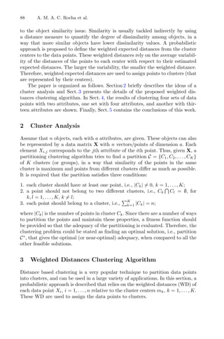
![A Simple Clustering Algorithm Based on Weighted Expected Distances 89
3.1 Weighted Expected Distances
To compute the WD between the data point Xi and center mk, we resort to the
distance vectors DVk, k = 1, . . . , K, and to the variations V ARk, k = 1, . . . , K,
the variability in cluster center mk relative to all data points. Thus, let DVk =
(DVk,1, DVk,2, . . . , DVk,n) be a n-dimensional distance vector that contains the
distances of data points X1, X2, . . . , Xn (a-dimensional vectors) to the cluster
center mk ∈ Ra
, where DVk,i = Xi − mk2 (i = 1, . . . , n). The componentwise
total of the distance vectors, relative to a particular data point Xi, is given by:
Ti =
K
k=1
DVk,i.
The probability of mk being surrounded and having a good centrality relative
to all points in the data set is given by
pk =
n
i=1 DVk,i
n
i=1 Ti
. (1)
Therefore, the expected value for the distance vector component i (relative to
point Xi) of the vector DVk is E[DVk,i] = pkTi. Then, the WD is defined for
each component i of the vector DVk, WD(k, i), using
WD(k, i) = DVk,i/V ARk (2)
(corresponding to the weighted distance assigned to data point Xi by the cluster
center mk), where the variation V ARk is the average amount of variability of
the distances of the points to the center mk, relative to the expected distances:
V ARk =
1
n
n
i=1
(DVk,i − E[DVk,i])
2
1/2
.
The larger the V ARk, the lower the weighted distances WD(k, i), i = 1, . . . , n
of the points relative to that center mk, when compared to the other centers.
A larger V ARk means that in average the difference between the estimated
expected distances and the real distances, to that center mk, is larger than to
the other centers.
3.2 The WD-Based Algorithm
Algorithm 1 presents the main steps of the proposed weighted expected distances
clustering algorithm. For initialization, a problem dependent number of clusters
is provided, e.g. K, so that the algorithm randomly selects K points from the
data set to initialize the cluster centers. To determine which data points are
assigned to a cluster, the algorithm uses the WD as a fitness function. Each
point Xi has a WD relative to a cluster center mk, the above defined WD(k, i).](https://image.slidesharecdn.com/optimizationlearningalgorithmsandapplications-231204021346-9e8015c0/85/Optimization-Learning-Algorithms-and-Applications-pdf-102-320.jpg)
![90 A. M. A. C. Rocha et al.
The lower the better. The minimization of WD(k, i) relative to k takes care of
the local property of the algorithm, assigning Xi to cluster Ck.
Algorithm 1. Clustering Algorithm
Require: data set X ≡ Xi,j, i = 1, . . . , n, j = 1, . . . , a, Itmax, Nmin
1: Set initial K; It = 1
2: Randomly select a set of K points from the data set X to initialize the K cluster
centers mk, k = 1, . . . , K,
3: repeat
4: Based on mk, k = 1, . . . , K, assign the data points to clusters and eventually
add a new cluster, using Algorithm 2
5: Compute ηD using (4)
6: Based on ηD, eventually remove clusters by merging two at a time, and remove
clusters with less than Nmin points, using Algorithm 3
7: Set m̄k ← mk, k = 1, . . . , K
8: Compute improved values for the cluster centers, mk, k = 1, . . . , K using Algo-
rithm 4
9: Set It = It + 1
10: until It Itmax or maxk=1,...,K m̄k − mk2 ≤ 1e − 3
11: return K∗
, mk, k = 1, . . . , K∗
and optimal C∗
= {C∗
1 , C∗
2 , . . . , C∗
K }.
Thus, to assign a point Xi to a cluster, the algorithm identifies the center
mk that has the lowest weighted distance value to that point, and if WD(k, i)
is inferior to the quantity 1.5ηk, where ηk is a threshold value for the center mk,
the point is assigned to that cluster. On the other hand, if WD(k, i) is between
1.5ηk and 2.5ηk a new cluster CK+1 is created and the point is assigned to CK+1;
otherwise, the WD(k, i) value exceeds 2.5ηk and the point is considered ‘noise’.
Thus, all points that have a minimum weighted distance to a specific center
mk between 1.5ηk and 2.5ηk are assigned to the same cluster CK+1, and if the
minimum weighted distances exceed 2.5ηk, the points are ‘noise’. The goal of
the threshold ηk is to define a bound to border the proximity to a cluster center.
The limit 1.5ηk defines the region of a good neighborhood, and beyond 2.5ηk the
region of ‘noise’ is defined. Similarity in the weighted distances and proximity
to a cluster center mk is decided using the threshold ηk. For each cluster k, the
ηk is found by using the average of the WD(k, .) of the points which are in the
neighborhood of mk and have magnitudes similar to each other. The similarity
between the magnitudes of the WD is measured by sorting their values and
checking if the consecutive differences remain lower that a threshold ΔW D. This
value depends on the number of data points and the median of the matrix WD
values (see Algorithm 2 for the details):
ΔW D =
n − 1
n
median[WD(k, i)]k=1,...,K, i=1,...,n. (3)
During the iterative process, clusters that are close to each other, measured
by the distance between their centers, may be merged if the distance between](https://image.slidesharecdn.com/optimizationlearningalgorithmsandapplications-231204021346-9e8015c0/85/Optimization-Learning-Algorithms-and-Applications-pdf-103-320.jpg)

![92 A. M. A. C. Rocha et al.
– adding a new cluster whose center is represented by the centroid of all points
that were not assigned to any cluster according to the rules previously defined;
– defining points ‘noise’ if they are not in an appropriate neighborhood of the
center that is closest to those points, or if they belong to a cluster with very
few points;
– merging clusters that are sufficiently close to each other, as well as removing
clusters with very few points.
On the other hand, the position of each cluster center can be iteratively
improved, by using the centroid of the data points that have been assigned to
that cluster and the previous cluster center [12,13], as shown in Algorithm 4.
Algorithm 3. Merging and Removing Clusters Algorithm
Require: K, mk, Ck, k = 1, . . . , K, ηD, Nmin, Xnoise
1: for k = 1 to K − 1 do
2: for l = k + 1 to K do
3: Compute Dk,l = mk − ml2
4: if Dk,l ≤ ηD then
5: Compute mk = 1
|Ck|+|Cl|
(|Ck|mk + |Cl|ml)
6: Assign all points X ∈ Cl to the cluster Ck
7: Delete ml (and remove Cl)
8: Update K
9: end if
10: end for
11: end for
12: for k = 1, . . . , K do
13: if |Ck| Nmin then
14: Define all X ∈ Ck as points ‘noise’ (add to class Xnoise)
15: Delete mk (remove Ck)
16: Update K
17: end if
18: end for
19: return K, mk, Ck for k = 1, . . . , K, and Xnoise.
Algorithm 4. Update Cluster Centers Algorithm
Require: mk, Ck, k = 1, . . . , K,
1: Update all cluster centers:
mk =
1
|Ck| + 1
⎛
⎝
Xl∈Ck
Xl + mk
⎞
⎠ for k = 1, . . . , K
2: return mk, k = 1, . . . , K](https://image.slidesharecdn.com/optimizationlearningalgorithmsandapplications-231204021346-9e8015c0/85/Optimization-Learning-Algorithms-and-Applications-pdf-105-320.jpg)
![A Simple Clustering Algorithm Based on Weighted Expected Distances 93
4 Computational Results
In this section, some preliminary results are shown. Four sets of data points
with two attributes, one set with four attributes (known as ‘Iris’) and one
set with thirteen attributes (known as ‘Wine’) are used to compute and visu-
alize the partitioning clustering. The algorithms are coded in MATLAB R
.
The performance of the Algorithm 1, based on Algorithm 2, Algorithm 3
and Algorithm 4, depends on some parameter values that are problem depen-
dent and dynamically defined: initial K = min{10, max{2, 0.01n}}, Nmin =
min{50, max{2, 0.05n}}, ΔW D 0, ηk 0, k = 1, . . . , K, ηD 0. The clus-
tering results were obtained for Itmax = 5, except for ‘Iris’ and ‘Wine’ where
Itmax = 20 was used.
4.1 Generated Data Sets
The generator code for the first four data sets is the following:
Problem 1. ‘mydata’1
with 300 data points and two attributes.
Problem 2. 2000 data points and two attributes.
mu1 = [1 2]; Sigma1 = [2 0; 0 0.5];
mu2 = [-3 -5]; Sigma2 = [1 0; 0 1];
X = [mvnrnd(mu1,Sigma1,1000); mvnrnd(mu2,Sigma2,1000)];
Problem 3. 200 data points and two attributes.
X = [randn(100,2)*0.75+ones(100,2); randn(100,2)*0.5-ones(100,2)];
Problem 4. 300 data points and two attributes.
mu1 = [1 2]; sigma1 = [3 .2; .2 2];
mu2 = [-1 -2]; sigma2 = [2 0; 0 1];
X = [mvnrnd(mu1,sigma1,200); mvnrnd(mu2,sigma2,100)];
In Figs. 1, 2, 3 and 4, the results obtained for Problems 1–4 are depicted:
– the plot (a) is the result of assigning the points (applying Algorithm 2) to
the clusters based on the initialized centers (randomly selected K points of
the data set);
– the plot (a) may contain a point, represented by the symbol ‘’, which iden-
tifies the position of the center of the cluster that is added in Algorithm 2
with the points that were not assigned (according to the previously referred
rule) to a cluster;
– plots (b) and (c) are obtained after the application of Algorithm 4 to update
the centers that result from the clustering obtained by Algorithm 2 and Algo-
rithm 3, at an iteration;
1
available at Mostapha Kalami Heris, Evolutionary Data Clustering in MATLAB
(URL: https://yarpiz.com/64/ypml101-evolutionary-clustering), Yarpiz, 2015.](https://image.slidesharecdn.com/optimizationlearningalgorithmsandapplications-231204021346-9e8015c0/85/Optimization-Learning-Algorithms-and-Applications-pdf-106-320.jpg)
![94 A. M. A. C. Rocha et al.
– the final clustering is visualized in plot (d);
– plots (a), (b), (c) or (d) may contain points ‘noise’ identified by the sym-
bol ‘×’;
– plot (e) shows the values of the Davies-Bouldin (DB) index, at each iteration,
obtained after assigning the points to clusters (according to the previously
referred rule) and after the update of the cluster centers;
– plot (f) contains the K-means clustering when K = K∗
is provided to the
algorithm.
The code that implements the K-means clustering [14] is used for comparative
purposes, although with K-means the number of clusters K had to be specified
in advance. The performances of the tested clustering algorithms are measured
in terms of a cluster validity measure, the DB index [15]. The DB index aims to
evaluate intra-cluster similarity and inter-cluster differences by computing
DB =
1
K
K
k=1
max
l=1,...,K, l=k
Sk + Sl
dk,l
(5)
where Sk (resp. Sl) represents the average of all the distances between the center
mk (resp. ml) and the points in cluster Ck (resp. Cl) and dk,l is the distance
between mk and ml. The smallest DB index indicates a valid optimal partition.
The computation of the DB index assumes that a clustering has been done.
The values presented in plots (a) (on the x-axis), (b), (c) and (d) (on the y-axis),
and (e) are obtained out of the herein proposed clustering (recall Algorithm 2,
Algorithm 3 and Algorithm 4). The values of the ‘DB index(m,X)’ and ‘CS
index(m,X)’ (on the y-axis) of plot (a) come from assigning the points to clusters
based on the usual minimum distances of points to centers. The term CS index
refers to the CS validity measure and is a function of the ratio of the sum of
within-cluster scatter to between-cluster separation [13]. The quantity ‘Sum of
Within-Cluster Distance (WCD)’ (in plots (b), (c) and (d) (on the x-axis)) was
obtained out of our proposed clustering process.
In conclusion, the proposed clustering is effective, very efficient and robust.
As it can be seen, the DB index values that result from our clustering are slightly
lower than (or equal to) those registered by the K-means clustering.
4.2 ‘Iris’ and ‘Wine’ Data Sets
The results of our clustering algorithm, when solving Problems 5 and 6 are now
shown. To compare the performance, our algorithm was run 30 times for each
data set.
Problem 5. ‘Iris’ with 150 data points. It contains three categories (types of
iris plant) with 4 attributes (sepal length, sepal width, petal length and petal
width) [16].
Problem 6. ‘Wine’ with 178 data points. It contains chemical analysis of 178
wines derived from 3 different regions, with 13 attributes [16].](https://image.slidesharecdn.com/optimizationlearningalgorithmsandapplications-231204021346-9e8015c0/85/Optimization-Learning-Algorithms-and-Applications-pdf-107-320.jpg)
![A Simple Clustering Algorithm Based on Weighted Expected Distances 95
-2 0 2 4 6 8
DB index = 1.4783
-2
-1
0
1
2
3
4
5
6
DB
index(m,X)
=
1.6035;
CS
index(m,X)
=
1.2197
Random selection of centers+Assign
Cluster 1
Cluster 2
Cluster 3
Cluster 4
(a) Assign after initialization
-2 0 2 4 6 8
Sum of Within-Cluster Distance (WCD) = 589.0572
-2
-1
0
1
2
3
4
5
6
BD
index
after
updating
centroids
=
0.96515
Assign+Delete+Update centroids, at iteration 1
Cluster 1
Cluster 2
Cluster 3
(b) 1st. iteration
-2 0 2 4 6 8
Sum of Within-Cluster Distance (WCD) = 379.0274
-2
-1
0
1
2
3
4
5
6
BD
index
after
updating
centroids
=
0.6342
Assign+Delete+Update centroids, at iteration 2
Cluster 1
Cluster 2
Cluster 3
(c) 2nd. iteration
-2 0 2 4 6 8
Sum of Within-Cluster Distance (WCD) = 374.6869
-2
-1
0
1
2
3
4
5
6
BD
index
after
updating
centroids
=
0.59976
Assign+Delete+Update centroids, at iteration 5
Cluster 1
Cluster 2
Cluster 3
(d) final clustering (5th iteration)
1 1.5 2 2.5 3 3.5 4 4.5 5
Iterations
0.5
0.6
0.7
0.8
0.9
1
1.1
1.2
1.3
1.4
1.5
Evaluation of new Updated Centers by DB index
DB index (After Update Centroids)
DB index (of Assign)
(e) DB index plot
-2 0 2 4 6 8
-2
-1
0
1
2
3
4
5
6
Kmeans, # clusters = 3 / DB index = 0.60831 / 5 iterations
Cluster 1
Cluster 2
Cluster 3
(f) K-means with K = 3
Fig. 1. Clustering process of Problem 1
The results are compared to those of [17], that uses a particle swarm opti-
mization (PSO) approach to the clustering, see Table 1. When solving the ‘Iris’
problem, our algorithm finds the 3 clusters in 77% of the runs (23 successful](https://image.slidesharecdn.com/optimizationlearningalgorithmsandapplications-231204021346-9e8015c0/85/Optimization-Learning-Algorithms-and-Applications-pdf-108-320.jpg)
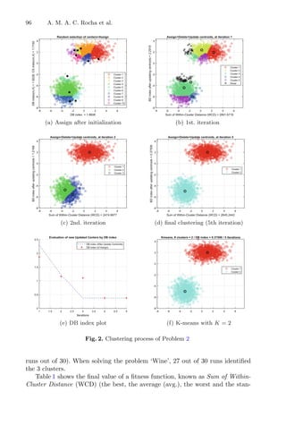
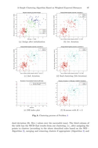
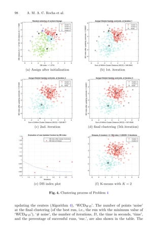
![A Simple Clustering Algorithm Based on Weighted Expected Distances 99
Table 1. Clustering results for Problems 5 and 6
Algorithm 1 Results in [17]
Problem ‘WCDW D’ # noise It Time suc. ‘WCD’ ‘WCD’ Time
‘Iris’ Best 107.89 0 5 0.051 77% 100.07 97.22 0.343
Avg. 108.21 8.7 0.101 100.17 97.22 0.359
Worst 109.13 12 0.156 100.47 97.22 0.375
St. Dev. 0.56 0.18
‘Wine’ Best 17621.45 0 6 0.167 90% 16330.19 16530.54 2.922
Avg. 19138.86 9.1 0.335 17621.12 16530.54 2.944
Worst 20637.04 13 1.132 19274.45 16530.54 3.000
St. Dev. 1249.68 1204.04
Table 2. Results comparison for Problems 5 and 6
Algorithm 1 K-means K-NM-PSO
Problem ‘WCDD’ # noise It Time suc. ‘WCD’ ‘WCD’
‘Iris’ Best 97.20 0 4 0.096 63% 97.33 96.66
Avg. 97.21 8.7 0.204 106.05 96.67
St. Dev. 0.01 14.11 0.008
‘Wine’ Best 16555.68 0 6 0.159 90% 16555.68 16292.00
Avg. 17031.79 10.3 0.319 18061.00 16293.00
St. Dev. 822.08 793.21 0.46
column identified with ‘WCD’ contains values of WCD (at the final clustering)
using X and the obtained final optimal cluster centers to assign the points to
the clusters/centers based on the minimum usual distances from each point to
the centers.
For the same optimal clustering, the ‘WCD’ has always a lower value than
‘WCDW D’. When comparing the ‘WCD’ of our clustering with ‘WCD’ registered
in [17], our obtained values are higher, in particular the average and the worst
values, except the best of the results ‘WCD’ for problem ‘Wine’. The variability
of the results registered in [17] and [18] (see also Table 2) are rather small but
this is due to the type of clustering based on the PSO algorithm. The clustering
algorithm K-NM-PSO [18] is a combination of K-means, the local optimization
method Nelder-Mead (NM) and the PSO. In contrast, our algorithm finds the
optimal clustering much faster than the PSO clustering approach in [17]. This
is a point in favor of our algorithm, an essential requirement when solving large
data sets.
The results of our algorithm shown in Table 2 (third column identified with
‘WCDD’) are based on the designed and previously described Algorithms 1,
2, 3 and 4, but using the usual distances between points and centers for the
assigning process (over the iterative process). These values are slightly better](https://image.slidesharecdn.com/optimizationlearningalgorithmsandapplications-231204021346-9e8015c0/85/Optimization-Learning-Algorithms-and-Applications-pdf-112-320.jpg)
![100 A. M. A. C. Rocha et al.
than those obtained by the K-means (available in [18]), but not as interesting as
those obtained by the K-NM-PSO (reported in [18]).
5 Conclusions
A probabilistic approach to define the weighted expected distances from the
cluster centers to the data points is proposed. These weighted distances are used
to assign points to clusters, represented by their centers. The new proposed
clustering algorithm relies on mechanisms to create new clusters. Points that are
not assigned to a cluster, based on the weighted expected distances, are gathered
in a new cluster. The clustering is also able to merge two nearby clusters and
remove the clusters that have very few points. Points are also identified as ‘noise’
when they are beyond a limit of a reasonable neighbourhood (as far as weighted
distances are concerned) and when they belong to a cluster with very few points.
The preliminary clustering results, and the comparisons with the K-means and
other K-means combinations with stochastic algorithms, show that the proposed
algorithm is very efficient and effective.
In the future, data sets with non-convex clusters, clusters with different
shapes, in particular those with non-spherical blobs, and sizes will be addressed.
Our proposal is to integrate a kernel function into our clustering approach. We
aim to further investigate the dependence of the parameter values of the algo-
rithm on the number of attributes, in particular, when highly dimensional data
sets should be partitioned. The set of tested problems will also be enlarged to
include large data sets with clusters of different shapes and non-convex.
Acknowledgments. The authors wish to thank three anonymous referees for their
comments and suggestions to improve the paper.
References
1. Jain, A.K., Murty, M.N., Flynn, P.J.: Data clustering: a review. ACM Comput.
Surv. 31(3), 264–323 (1999)
2. Greenlaw, R., Kantabutra, S.: Survey of clustering: algorithms and applications.
Int. J. Inf. Retr. Res. 3(2) (2013). 29 pages
3. Ezugwu, A.E.: Nature-inspired metaheuristics techniques for automatic clustering:
a survey and performance study. SN Appl. Sci. 2, 273–329 (2020)
4. Mohammed, J.Z., Meira, W., Jr.: Data Mining and Machine Learning: Fundamen-
tal Concepts and Algorithms, 2nd edn. Cambridge University Press, Cambridge
(2020)
5. Xu, D., Tian, Y.: A comprehensive survey of clustering algorithms. Ann. Data Sci.
2(2), 165–193 (2015)
6. MacQueen, J.B.: Some methods for classification and analysis of multivariate obser-
vations. In: Le Cam, L.M., Neyman, J. (eds.) Proceedings of the Fifth Berkeley
Symposium on Mathematical Statistics and Probability, vol. 1, pp. 281–297. Uni-
versity of California Press (1967)
7. Manning, C.D., Raghavan, P., Schütze, H.: Introduction to Information Retrieval.
Cambridge University Press, Cambridge (2008)](https://image.slidesharecdn.com/optimizationlearningalgorithmsandapplications-231204021346-9e8015c0/85/Optimization-Learning-Algorithms-and-Applications-pdf-113-320.jpg)

![Optimization of Wind Turbines
Placement in Offshore Wind Farms:
Wake Effects Concerns
José Baptista1,2(B)
, Filipe Lima1
, and Adelaide Cerveira1,2
1
School of Science and Technology, University of Trás-os-Montes and Alto Douro,
5000-801 Vila Real, Portugal
{baptista,cerveira}@utad.pt, al64391@utad.eu
2
UTAD’s Pole, INESC-TEC, 5000-801 Vila Real, Portugal
Abstract. In the coming years, many countries are going to bet on
the exploitation of offshore wind energy. This is the case of southern
European countries, where there is great wind potential for offshore
exploitation. Although the conditions for energy production are more
advantageous, all the costs involved are substantially higher when com-
pared to onshore. It is, therefore, crucial to maximize system efficiency.
In this paper, an optimization model based on a Mixed-Integer Linear
Programming model is proposed to find the best wind turbines loca-
tion in offshore wind farms taking into account the wake effect. A case
study, concerning the design of an offshore wind farm, were carried out
and several performance indicators were calculated and compared. The
results show that the placement of the wind turbines diagonally presents
better results for all performance indicators and corresponds to a lower
percentage of energy production losses.
Keywords: Offshore wind farm · Wake effect · Optimization
1 Introduction
In the last two decades, wind energy has been a huge investment for almost
all developed countries, with a strong bet on onshore wind farms (WF). It is
expected that investments will be directed towards the energy exploration in
the sea, where offshore wind farms (OWFs) are a priority. Recently, the Euro-
pean Union has highlighted the enormous unexplored potential in Europe’s seas,
intending to multiply offshore wind energy by 20 to reach 450 GW, to meet the
objective of decarbonizing energy and achieving carbon neutrality by 2050 [6].
An OWF has enormous advantages over onshore, with reduced visual impact
and higher efficiency, where the absence of obstacles allow the wind to reach a
higher and more constant speed. However, the installation costs are substan-
tially higher [10]. So, it is very important to optimize the efficiency of these
c
Springer Nature Switzerland AG 2021
A. I. Pereira et al. (Eds.): OL2A 2021, CCIS 1488, pp. 102–109, 2021.
https://doi.org/10.1007/978-3-030-91885-9_8](https://image.slidesharecdn.com/optimizationlearningalgorithmsandapplications-231204021346-9e8015c0/85/Optimization-Learning-Algorithms-and-Applications-pdf-115-320.jpg)
![Optimization of WT Placement in OWF: Wake Effects Concerns 103
WFs, wherein the location of wind turbines (WTs) is one of the most important
factors to consider, taking into account the wake effect impact on the energy
production of each one. To achieve this goal new models related to WF layout
optimization should be investigated. Several authors addressed the topic using
models based on genetic algorithms (GA) as is the case of Grady et al. [7]. In
[12], a mathematical model based in a particle swarm optimization (PSO) algo-
rithm which includes the variation of both wind direction and wake deficit is
proposed. A different approach is addressed in [13], where a modular framework
for the optimization of an OWF using a genetic algorithm is presented. In [14]
a sequential procedure is used for global optimization consisting of two steps:
i) a heuristic method to set an initial random layout configuration, and ii) the
use of nonlinear mathematical programming techniques for local optimization,
which use the random layout as an initial solution. Other authors address the
topic of WF optimization, focusing on optimizing the interconnection between
the turbines, known as cable routing optimization. Cerveira et al. in [5] pro-
poses a flow formulation to find the optimal cable network layout considering
only the cable infrastructure costs. In [3,4,11] Mixed-Integer Linear Program-
ming (MILP) models are proposed to optimize the wind farm layout in order
to obtain the greater profit of wind energy, minimizing the layout costs. Assum-
ing that the ideal position of the turbines has already been identified, the most
effective way of connecting the turbines to each other and to the substations,
minimizing the infrastructure cost and the costs of power losses during the wind
farm lifetime is considered.
The main aim of this paper is to optimize the location of the WTs to minimize
the single wake effect and so to maximize energy production. In order to achieve
this target, a MILP optimization model is proposed. A case study is considered
and performance indicators were computed and analyzed obtaining guidelines
for the optimal relative position of the WTs. The paper is organized as follows.
In Sect. 2 the wind power model is addressed and in Sect. 3 the MILP model
to optimize the WTs placement is presented. Section 4 presents the case study
results. Finally, Sect. 5 highlights some conclusions remarks.
2 Wind Farm Power Model
A correct evaluation of the wind potential for power generation must be based
on the potential of the wind resource and various technical and physical aspects
that can affect energy production. Among them, the wind speed probability
distribution, the effect of height, and the wake effect are highlighted.
2.1 Power in the Wind
The energy available for a WT is kinetic energy associated with an air column
traveling at a uniform and constant speed u, in m/s. The power available in the
wind, in W, is proportional to the cube of the wind speed, given by Eq. (1),
P =
1
2
(ρAv)v2
=
1
2
ρAv3
(1)](https://image.slidesharecdn.com/optimizationlearningalgorithmsandapplications-231204021346-9e8015c0/85/Optimization-Learning-Algorithms-and-Applications-pdf-116-320.jpg)
![104 J. Baptista et al.
where A is the swept area by the rotor blades, in m2
, v is the wind speed, in
m/s, and ρ is the air density, usually considered as constant during the year, with
standard value being equal to 1.225 kg/m3
. The power availability significantly
depends on the wind speed, so, it is very important to place the turbines where
the wind speed is high. Unfortunately, the total wind power cannot be recovered
in a WT. According to Betz law [2], it is only allowed to convert, at most,
59.3% of the kinetic energy in mechanical energy to be used through the turbine.
Typically, turbines’ technical is provided by manufacturers. This is the case of
the power curve which gives the electrical power output, Pe(v), as a function of
the wind speed, v. Knowing the wind profile and the turbine power curve, it is
possible to determine the energy Ea produced by the conversion system,
Ea = 8760
vmax
v0
f(v)Pe(v)dv. (2)
2.2 The Jensen Model for Wake Effect
The power extraction of turbines from the wind depends on the wind energy
content, which differs in its directions. The downstream wind (the one that
comes out of the turbine) has less energy content than the upstream wind. The
wake effect is the effect of upstream wind turbines on the speed of the wind that
reaches downstream turbines. In a WF where there are several WTs, it is very
likely that the swept area of a turbine is influenced by one or more turbines
that are before, this effect can be approached by the Jensen model proposed in
1983 by N. O. Jensen [8] and developed in 1986 by Katic et al. [9]. The initial
diameter of the wake is equal to the diameter of the turbine and expands linearly
as a function of wind. Similarly, the downstream wind deficit declines linearly
with the distance to the turbine. The simple wake model consists of a linear
expression of the wake diameter and the decay of the speed deficit inside the
wake. The downstream wind speed (vd) of the turbine can be obtained by (3),
where v0 represents the upstream wind speed.
vd = v0
⎛
⎜
⎝1 −
N
i=1
2a
(1 + αx
r1
)2
2
⎞
⎟
⎠ (3)
Where: the wake radius r1 is given by r1 = αx + rr, in which rr is the radius of
the upstream turbine; x is the distance that meets the obstacle; α is a scalar that
determines how quickly the wake expands, which is given by α = 1
2 ln z
z0
, where
z is the hub height and z0 is the surface roughness that in the water is around
0.0002 m, although it may increase with sea conditions; a is the axial induction
factor given by a = (1 −
√
1 − CT )/2, and the turbine thrust coefficient CT is
determined by the turbine manufacturer according to Fig. 1.](https://image.slidesharecdn.com/optimizationlearningalgorithmsandapplications-231204021346-9e8015c0/85/Optimization-Learning-Algorithms-and-Applications-pdf-117-320.jpg)
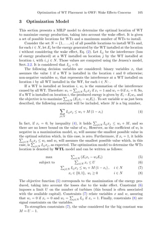
![106 J. Baptista et al.
4 Case Study and Results
In this section, a case study will be described and the results are presented and
discussed. The WT used was Vestas v164-8.0 [15] with the power curve provided
by the manufacturer shown in Fig. 1. The site chosen for the WT installation
is approximately 20 km off the coast of Viana do Castelo, Portugal, location
currently used by the first Portuguese OWF. To achieve the average annual
wind speed there was used the Global wind Atlas [1] data. The average annual
wind speed considered at the site was 8 m/s collected at 150 m of height. Prandtl
Law was used to extrapolate the wind speed at the turbine hub height, around
140 m. Subsequently, the annual frequency of occurrence is calculated for various
wind speeds, in the range between 4 m/s and 25 m/s (according to the WT power
curve), using the Rayleigh distribution. The occurrence of these wind speeds is
shown in the bar chart of Fig. 2a. Figure 2b shows the annual energy production
of a WT at each wind speeds considered. Adding all energy values, the total
yearly energy production for this WT will be 29.1 GWh.
Fig. 1. Power and thrust coefficient curve for WT Vestas V164-8.0.
(a) Number of hours wind speeds occur. (b) Annual energy produced by a WT.
Fig. 2. Wind distribution and annual energy production.
There are 36 possible locations for WT, distributed over six rows, each one of
them having six possible locations, as shown in Fig. 3a. The horizontally and ver-
tically distance between two neighbored locations is 850 m and the predominant
wind direction is marked with an arrow.](https://image.slidesharecdn.com/optimizationlearningalgorithmsandapplications-231204021346-9e8015c0/85/Optimization-Learning-Algorithms-and-Applications-pdf-119-320.jpg)
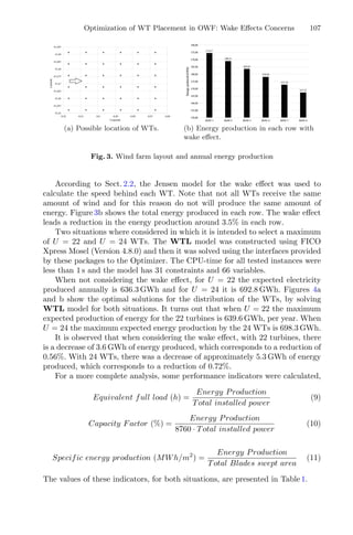
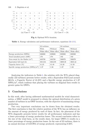

![A Simulation Tool for Optimizing a 3D Spray Painting System 111
2 Literature Review
Spray painting simulation is an important part of automated spray painting sys-
tems since it provides the possibility to predict the end result without any cost.
Furthermore, virtual simulations allow quality metrics such as paint thickness
uniformity or paint coverage to be easily measured and optimized. This section
analyse the basis to simulate spray painting, including painting methods and sev-
eral approaches on the spray simulation, such as computational fluid dynamics
(CFD), spray simulation applied to robotics and commercial simulators.
2.1 Painting Methods
Paint application has been used for centuries, for most of this time the main
methods consisted in spreading paint along the desired surface with tools like
a brush or a roller. Nowadays however, their popularity and use are decreasing
since they are slow methods with low efficiency, and the resulting quality highly
depends on the quality of the materials and tools. Consequently new techniques
were developed such as dipping and flow coating, that are best applied to small
components and protective coatings, and spray painting that is more suitable
for industry.
The main industrial painting methods are: air atomized spray application,
high volume low pressure (HVLP) spray application, airless spray application,
air-assisted airless spray application, heated spray application and electrostatic
spray application [19].
The conventional spray application method is air atomized spray. In this
method the compressed air is mixed with the paint in the nozzle and the atomized
paint is propelled out of the gun. HVLP is an improvement on the conventional
system and is best suited for finishing operations. The paint is under pressure and
the atomization occurs when it contacts with the high volume of low pressure air
resulting in the same amount of paint to be propelled at the same rate but with
lower speeds. This way a high precision less wasteful spray is produced, since
the paint doesn’t miss the target and the droplets don’t bounce back. Airless
spray application is a different method, that uses a fluid pump to generate high
pressure paint. The small orifice in the tip atomizes the pressurized paint. The
air resistance slows down the droplets and allows for a good amount to adhere to
the surface, but still in a lower extent than HVLP [14]. Air-assisted airless spray
application is a mixture of the airless and conventional methods with the purpose
of facilitating the atomization and decreasing the waste of paint. Heated spray
application can be applied to the other methods and it consists in pre-heating
the paint, making it less viscous requiring lower pressures. This also reduces
drying time and increases efficiency. Electrostatic spray application can also be
applied with the other techniques and consists in charging the paint droplets as
they pass through an electrostatic field. The surface to be painted is grounded
in order to attract the charged particles [18].
At last, the conditions at which the paint is applied have a direct impact on
the paint job quality and success. This way, painting booths are usually used,](https://image.slidesharecdn.com/optimizationlearningalgorithmsandapplications-231204021346-9e8015c0/85/Optimization-Learning-Algorithms-and-Applications-pdf-124-320.jpg)
![112 J. Casanova et al.
because it is easier to control aspects such as temperature, relative humidity
and ventilation. Lower temperatures increase drying time, while high moisture
in the air interferes with adhesion and can cause some types of coating not to
cure. Also the ventilation decreases initial drying time and allows the workspace
to be safer for the workers.
2.2 Computational Fluid Dynamics (CFD)
In order to simulate the spray painting process as accurately as possible, it is
necessary to understand the physical properties that dictate droplets trajecto-
ries and deposition. Computational fluid dynamics (CFD) allows for a numerical
approach that can predict flow fields using the Navier-Stokes equations [15]. An
important step that CFD still struggles to solve is the atomization process. It
is possible to skip the atomization zone by using initial characteristics that can
be approximated by measures of the spray [16]. Another alternative is to allow
some inaccuracies of the model in the atomization zone by simulating completed
formed droplets near the nozzle. This allows for simpler initialization while main-
taining accurate results near the painted surface [21]. The Fig. 1 shows a CFD
result that compared with the experimental process reveals similar thickness
[22].
Despite these advantages, CFD isn’t used in industrial applications [11]. This
is due to the fact that CFD requires a high computation cost and the precision
that it produces isn’t a requirement for many applications. On the other hand,
with the current technological advances this seems to be a promising technique
that enables high precision even on irregular surfaces [20].
Fig. 1. CFD results with the calculated velocity contours colored by magnitude (m/s)
in the plane z = 0 [22].](https://image.slidesharecdn.com/optimizationlearningalgorithmsandapplications-231204021346-9e8015c0/85/Optimization-Learning-Algorithms-and-Applications-pdf-125-320.jpg)
![A Simulation Tool for Optimizing a 3D Spray Painting System 113
Fig. 2. On the left side is presented a beta distribution for varying β [11]. On the right
side is presented an asymmetrical model (ellipse) [11].
2.3 Spray Simulation Applied to robotics
In robotics, it is common to use explicit functions to describe the rate of paint
deposition at a point based on the position and orientation of the spray gun.
Depending on the functions used, it is conceivable to create finite and infinite
range models [11]. In infinite range models the output approaches zero as the
distance approaches infinity. The most usually used distributions are Cauchy and
Gaussian. Cauchy is simpler, allowing for faster computation while Gaussian is
rounder and closer to reality [10,17]. It is also possible to use multiple Gaussian
functions in order to obtain more complex and accurate gun models [24]. If the
gun model is considerably asymmetrical, an 1D Gaussian with an offset revolved
around an axis summed with a 2D Gaussian provides a 2D deposition model [13].
In finite range models the value of deposition outside a certain distance is actu-
ally zero. Several models have been developed such as trigonometric, parabolic,
ellipsoid and beta [11]. The most used model is the beta distribution model that,
as the beta increases, changes from parabolic to ellipsoid and even the Gaussian
distribution can be modelled, as shown in Fig. 2 [9]. It is also useful to use two
beta distributions that best describe the gun model, as was done with infinite
range models, Fig. 2 exemplifies an asymmetrical model [23].
2.4 Commercial Simulators
The growing necessity of an user friendly software that provides a fast and
risk free way of programming industrial manipulators led to the development of
dedicated software by the manipulators manufacturers and by external software
companies. Most of them include essential features such as support for several
robots, automatic detection of axis limits, collisions and singularities and cell
components positioning.](https://image.slidesharecdn.com/optimizationlearningalgorithmsandapplications-231204021346-9e8015c0/85/Optimization-Learning-Algorithms-and-Applications-pdf-126-320.jpg)
![114 J. Casanova et al.
RoboDK is a software developed for industrial robots that works as an offline
programming and simulation tool [3]. With some simple configurations it’s pos-
sible to simulate and program a robotic painting system, however the simulation
is a simple cone model and the programming is either entered manually or a
program must be implemented [4]. This is a non trivial task for the end user
but a favorable feature for research in paint trajectory generation. The advan-
tages of this system are mainly the possibility to create a manual program and
experiment it without any danger of collisions or without any waste of paint.
RobCad paint, by Siemens, also works as an offline programming and simulation
tool and also presents features as paint coverage analysis and paint databases
[7]. It also includes some predefined paths that only require the user to set a
few parameters. This simulator is one of the oldest in the market being used by
many researchers to assess their algorithms. OLP Automatic by Inropa is a sys-
tem that uses 3D scanning to automatically produce robot programs [1]. A laser
scanner is used to scan parts that are placed on a conveyor and the system can
paint every piece without human intervention. Although there are no available
information about the created paths, the available demonstrations only paint
simple pieces like windows and doors. Delfoi Paint is an offline programming
software that besides the simulation and thickness analysis tools has distinctive
features such as pattern tools that create paths based on surface topology and
manual use of the 3D CAD features [2]. RoboGuide PaintPRO by FANUC, on
the other hand is specifically designed to generate paths for FANUC robots [8].
The user selects the area to be painted and chooses the painting method and
the path is generated automatically. Lastly, RobotStudio R
Paint PowerPac by
ABB is purposely developed for ABB robots and doesn’t have automatically
generated paths. Its main benefit is the fast development of manual programs
for multiple simultaneous robots.
3 Simulator Painting Add-On
The simulation was developed as an additional feature on an already existing
robotics simulator, SimTwo. SimTwo is robot simulation environment that was
designed to enable researchers to accurately test their algorithms in a way that
reflected the real world. SimTwo uses The Open Dynamics Engine for simulat-
ing rigid body dynamics and the virtual world is represented using GLScene
components [5], these provide a simple implementation of OpenGL [6].
In order to simulate the spray painting, it is taken the assumption that the
target model has regular sized triangles. As this is rarely the case, a preprocess
phase is required, where the CAD model is remeshed using an Isotropic Explicit
Remeshing algorithm that repeatedly applies edge flip, collapse, relax and refine](https://image.slidesharecdn.com/optimizationlearningalgorithmsandapplications-231204021346-9e8015c0/85/Optimization-Learning-Algorithms-and-Applications-pdf-127-320.jpg)
![A Simulation Tool for Optimizing a 3D Spray Painting System 115
Fig. 3. On top is presented the car hood model produced by the modeling software.
On the bottom is presented the same model after the Isotropic Explicit Remeshing.
to improve aspect ratio and topological regularity. This step can be held by the
free software MeshLab [12] and the transformation can be observed in Fig. 3 with
a CAD model of a car hood as an example.
The importance of the preprocess lies in the fact that from thereafter the
triangle center describes a triangle location, since the triangles are approximately
equilateral. Another important result emerges from the fact that every triangle
area is identical and small enough so that each triangle constitutes an identity
for the mesh supporting a pixel/vortex like algorithm.](https://image.slidesharecdn.com/optimizationlearningalgorithmsandapplications-231204021346-9e8015c0/85/Optimization-Learning-Algorithms-and-Applications-pdf-128-320.jpg)
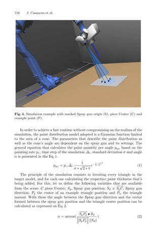

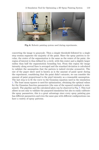
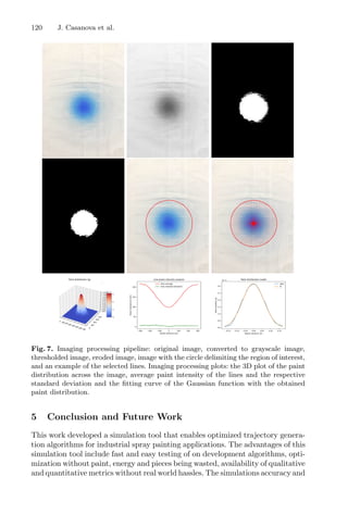


![124 J. Fernandes et al.
1 Introduction
Speech pathologies are relatively common and can be found in different stages of
evolution and severity, affecting approximately 10% of the population [1]. These
pathologies directly affect vocal quality, as they alter the phonation process and
have increased dramatically in recent times, mainly due to harmful habits, such
as smoking, excessive consumption of alcoholic beverages, persistent inhalation
of dust-contaminated air and abuse of voice [2].
There are a variety of tests that can be performed to detect pathologies
associated with the voice, however, they are invasive becoming uncomfortable
for patients and are time-intensive [3].
Auditory acoustic analyzes, performed by professionals, lack objectivity and
depend on the experience of the physician who makes the assessment. Acoustic
analysis allows non-invasively to determine the individual’s vocal quality. It is a
technique widely used in the detection and study of voice pathologies, since it
allows to measure properties of the acoustic signal of a recorded voice where a
speech or vowels are said in a sustained way [4,5]. This analysis is able to provide
the sound wave format allowing the evaluation of certain characteristics such as
frequency disturbance measurements, amplitude disturbance measurements and
noise parameters.
Jitter is one of the most used parameters as part of a voice exam and is used
by several authors Kadiri and Alku 2020 [6], Teixeira et al. 2018 [7], Sripriya
et al. 2017 [8], Teixeira and Fernandes 2015 [9] to determine voice pathologies.
Jitter is the measure of the cycle to cycle variations of the successive glottic
cycles, being possible to measure in absolute or relative values. Jitter is mainly
affected by the lack of control in the vibration of the vocal folds. Normally, the
voices of patients with pathologies tend to have higher values of jitter [10].
This work intends to improve the algorithm developed by Teixeira and
Gonçalves [10,11] to obtain the jitter parameter, to later be used in a com-
plementary diagnostic system and obtain realiable jitter values. As a means of
reference, to ensure reliable values of the algorithm, Praat is used as a refer-
ence for comparison, as this software is accepted by the scientific community as
an accurate measure and is open software. This software is developed by Paul
Boersma and David Weenink [12], from the Institute of Phonetic Sciences at the
University of Amsterdam.
This article is organized as follows: Sect. 2 describes the determination of the
absolute jitter, the pathologies and the database used, as well as the number
of subjects used for the study; Sect. 3 describes some of the problems found
in some signals in the Teixeira and Gonçalves algorithms [10,11], as well as
the description and flowchart of the adjusted algorithm; Sect. 4 describes the
studies carried out, the results obtained and the discussion. Finally, in Sect. 5
the conclusions are presented.](https://image.slidesharecdn.com/optimizationlearningalgorithmsandapplications-231204021346-9e8015c0/85/Optimization-Learning-Algorithms-and-Applications-pdf-137-320.jpg)
![Optimization of Glottal Onset Peak Detection 125
2 Methodology
In Fig. 1, the jitter concept is illustrated, where it is possible to perceive that
jitter corresponds to the measure of the variation of the duration of the global
periods.
Fig. 1. Jitter representation in a sustained vowel /a/.
2.1 Jitter
Jitter is defined as a measure of glottal variation between cycles of vibration of
the vocal cords. Subjects who cannot control the vibration of the vocal cords
tend to have higher values of jitter [11].
Absolute jitter (jitta) is the variation of the glottal period between cycles,
that is, the average absolute difference between consecutive periods, expressed
by Eq. 1.
jitta =
1
N − 1
N
i=2
|Ti − Ti−1| (1)
In Eq. 1 Ti is the size of the glottal period i and N is the total number of glottal
periods.
2.2 Database
The German Saarbrucken Voice Database (SVD) was used. This database is
available online by the Institute of Phonetics at the University of Saarland [13].
The database consists of voice signals of more than 2000 subjects with several dis-
ease and controls/healthy subjects. Each person has the recording of phonemes
/a/, /i/ and /u/ in the low, normal and high tones, swipe along tones, and the](https://image.slidesharecdn.com/optimizationlearningalgorithmsandapplications-231204021346-9e8015c0/85/Optimization-Learning-Algorithms-and-Applications-pdf-138-320.jpg)
![126 J. Fernandes et al.
German phrase “Guten Morgen, wie geht es Ihnen?” (“Good morning, how are
you?”). The size of the sound files is between 1 and 3 s and have a sampling
frequency of 50 kHz.
For the analysis it was used a sub-sample of 10 control subjects (5 male and
5 female) and 5 patient subjects (2 male and 3 female), of 3 diseases. Of these,
2 subjects had chronic laryngitis, one of each gender, 2 subjects with vocal cord
paralysis, one of each gender and 1 female with vocal cord polyps.
3 Development
3.1 Comparative Analysis Between the Signals Themselves
Teixeira and Gonçalves in [11] reported the results of the algorithm using groups
of 9 healthy and 9 pathological male and female subject. The authors compared
the average measures of the algorithm and Praat software, over the groups of 9
subjects. The comparison shows generally slightly higher values measured by the
algorithm, but with difference lower than 20 µs except for the female pathological
group. 20 µs corresponds to only one speech signal sample at 50 kHz sampling
frequency. Authors claim a difference lower than 1 speech sample in average.
Anyhow, in a particular speech file it was found very high differences between
the algorithm measures and the Praat measures.
In order to try to understand why the jitter measure in some particular
speech files of the Teixeira and Gonçalves 2016 [11] algorithm are so different
from the reference values, we proceeded to a visual comparison of the signals in
the reference software and in the Teixeira and Gonçalves 2016 algorithm.
In this way, we took the signals in which the values for absolute jitter were
very different and it was noticed that for a particular shapes of the signal the
algorithm do not find the peaks in a similar way as Praat did.
In a female control signal, the reference value for absolute jitter was 10.7 µs
and the algorithm value was 478.6 µs. When the signal was observed, it was
realized that one of the reasons that led to this difference was the fact that the
algorithm was selecting the maximum peaks to make the measurement, while the
reference software was using the minimum peaks. This led us to try to understand
why the algorithm is selecting the maximum peaks, instead of selecting the
minimums. The conclusion observed in Fig. 2 was reached.
As it can be seen in Fig. 2, the algorithm is finding two maximum values
for the same peak. This first search of peaks is taken in a initial phase of the
algorithm to decide to use the maximum or minimum peaks. This two close
peaks leads the algorithm to erroneously choose the peaks it will use to make the
measurement, since it does not satisfy the condition of the algorithm (number of
maximum peaks = 10, in a 10 glottal periods length part of speech). This problem
occurs in more signals. Correcting this error, for this signal, the absolute jitter
value went from 478.6 µs to 39.3 µs.
In another signal, also from a control subject, in which the reference value
for the absolute jitter is 9.6 µs and the value of the algorithm was 203,1 µs.](https://image.slidesharecdn.com/optimizationlearningalgorithmsandapplications-231204021346-9e8015c0/85/Optimization-Learning-Algorithms-and-Applications-pdf-139-320.jpg)
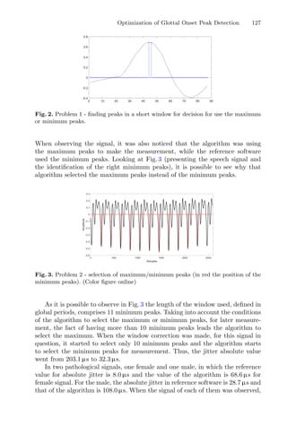
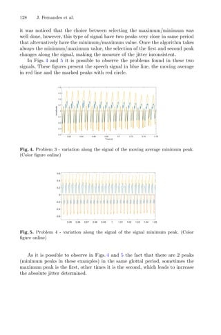
![Optimization of Glottal Onset Peak Detection 129
3.2 Algorithm Adjustments
The main purpose of the present work is to present the optimizations applied to
the algorithm proposed in [11], since it was mainly observed the inability to deal
with some recordings, both in the control group and those who have some type of
pathology. Thus, a recap of the steps in [11] is proposed in order to contextualize
each improvement developed. It must be emphasised the importance of the exact
identification of the position of each onset time of the glottal periods, for an
accurate measure of the Jitter values. The onset time of the glottal periods are
considered as the position of the peaks in the signal.
According to [11], the process of choosing the references for calculating the
Jitter parameter can be better performed by analyzing the signal from its cen-
tral region. There it is expected to find high stationarity. In addition, it was
concluded that a window of 10 fundamental periods contains enough informa-
tion to determine the reference of the length of the fundamental period and the
selection between the minimums or maximums. On this window, the moments
that occur the positive and negative peaks of each glottal period are determined,
as well as the amplitude module of the first cycle. The step between adjacent
cycles is based on the peak position of the previous cycle plus a fundamental
period. Focusing on this point, the position of the posterior peak is determined
by searching for the maximum (or minimum) over a two-third window of the
fundamental period. Finally, in an interval of two fifths of fundamental period,
around each peak, the search for other peaks corresponding to at least 70% of
its amplitude is carried out. The reference determination is made considering
the positive and negative amplitudes of the first module cycle and the count of
positive and negative peaks in the interval of 10 cycles. Basically, the measure of
amplitude directs the decision to the parameter with the greatest prominence,
since it is expected to have isolated peaks for the one with the greatest ampli-
tude. On the other hand, the count of cycles indicates the number of points
and oscillations close to the peaks, which may eventually prevail over these. The
occurrence of these behaviors may or may not be something characteristic of the
signal, in a way that it was observed that for cases in which this rarely occurred,
a slight smoothing should be sufficient to readjust the signal. In [11], when the
peak count exceeded the limit of 10 for both searches, a strong smoothing was
applied over the signal that sometimes de-characterized it.
Based on the mentioned amplitude parameters and the peaks count, a
decision-making process is carried out, which concludes with the use of max-
imums or minimums of the original signal or its moving average, to determine
all glottal periods. In Fig. 6 the flowchart of the proposed algorithm is presented.](https://image.slidesharecdn.com/optimizationlearningalgorithmsandapplications-231204021346-9e8015c0/85/Optimization-Learning-Algorithms-and-Applications-pdf-142-320.jpg)
![130 J. Fernandes et al.
Fig. 6. Algorithm flowchart.
The rules of the decision process are described below, where the limit param-
eter n = 13 is defined as the maximum peak count accepted for the use of the
original signal or for the application of light straightening.
• If the maximum amplitude is greater than the minimum amplitude in module
and the maximum peak count is in the range [10, n], or, the minimum peak
count is greater than n and the maximum peak count is in [10, n]:
◦ If the maximum count is equal to 10, the search for peaks is per-
formed on the original signal using the maximum as a cycle-by-cycle
search method;
◦ Else, a moving average with a Hanning window of equal length to a
ninth of a fundamental period is applied to the signal and the search for
peaks in this signal is carried out through the maximum of each cycle.
Figure 7 shows the comparison between the original signals, the moving](https://image.slidesharecdn.com/optimizationlearningalgorithmsandapplications-231204021346-9e8015c0/85/Optimization-Learning-Algorithms-and-Applications-pdf-143-320.jpg)
![Optimization of Glottal Onset Peak Detection 131
average MA1 and the moving average MA2. The peak marking was per-
formed within this rule, that is, starting from MA1 and using maximum
method. It is noted that the slight smoothing applied keeps the peak
marking close to the real one and maintains, in a way, the most signifi-
cant undulations of the signal, whereas MA2, in addition to shifting the
position of the peaks more considerably, their undulations are composed
of the contribution of several adjacent waves. This can reduce the reli-
ability of marking signals that have peaks’ side components with high
amplitude in modulus.
Fig. 7. Comparison between the original signal, the signal after moving average with
Hanning window of length N0/9 (MA1) and the signal after moving average with
Hanning window of length N0/3 (MA2). The peaks of glotal periods are shown in
black and were detected through maximum method over MA1. Recording excerpt from
a healthy subject performing /i/ low. Normalized representation.
• Else, if the minimum amplitude in module is greater than the maximum
amplitude and the minimum peak count is in the range [10, n], or, the max-
imum peak count is greater than n and the minimum peak count is in [10,
n]:
◦ If the minimum count is equal to 10, the search for peaks is per-
formed on the original signal using the minimum as a cycle-by-cycle search
method;
◦ Else, a moving average with a Hanning window of equal length to a
ninth of a fundamental period is applied to the signal and the search for
peaks in this signal is carried out through the minimum of each cycle.
Figure 8 shows an example of the path taken through this rule. Here, the
generated MA1 signal proves to be much less sensitive than the MA2 (gen-
erated for comparison) since in this one, the wave that contains the real
peak is strongly attenuated by the contribution of the previous positive
amplitude to the averaging. In this way, the application of smoothing](https://image.slidesharecdn.com/optimizationlearningalgorithmsandapplications-231204021346-9e8015c0/85/Optimization-Learning-Algorithms-and-Applications-pdf-144-320.jpg)
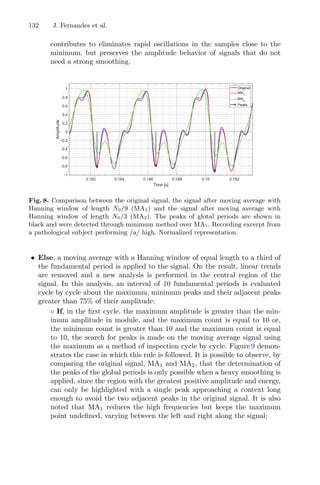
![Optimization of Glottal Onset Peak Detection 133
Fig. 9. Comparison between the original signal, the signal after moving average with
Hanning window of length N0/9 (MA1) and the signal after moving average with
Hanning window of length N0/3 (MA2). The peaks of glotal periods are shown in
black and were detected through maximum method over MA2. Recording excerpt from
a pathological subject performing /a/ normal. Normalized representation.
◦ Else, the search for peaks is done on the moving average signal using
the minimum as a method of inspection cycle by cycle.
In all cases, the inspection of the peaks cycle by cycle of every signal is carried
out with steps of a fundamental period from the reference point (maximum
or minimum) and then an interval of one third of the fundamental period is
analyzed. The reduction in the length of this interval from two thirds (used in
[11]) to one third makes the region of analysis more restricted to samples close
to one step from the previous peak. With this it is expected to guarantee that
the analysis is always carried out in the same region of the cycles, avoiding the
exchange between adjacent major peaks. However, in the cases where there is a
shift in the fundamental frequency over time, the use of a fixed parameter as a
step between cycles, as done in [11] and in this work, can cause inevitable errors
in the definition of the search interval. The maximum or minimum points of
each cycle are used as a source for determining the parameters Jitter according
to Eqs. 1.
4 Results and Discussion
In this section, the results of some analyzes made will be reported, as well as
their discussion.
A comparative analysis was made for the values of absolute jitter between
the values obtained by the algorithm developed by Teixeira and Gonçalves 2016
[11], the reference software [12] and the adjusted algorithm, in order to try
to understand if the adjusted algorithm values are closer to the values of the](https://image.slidesharecdn.com/optimizationlearningalgorithmsandapplications-231204021346-9e8015c0/85/Optimization-Learning-Algorithms-and-Applications-pdf-146-320.jpg)
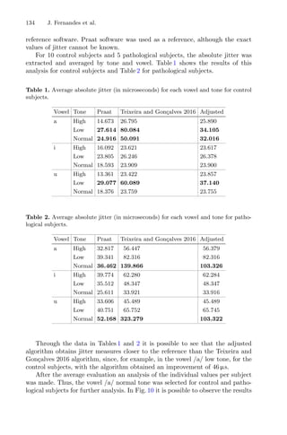
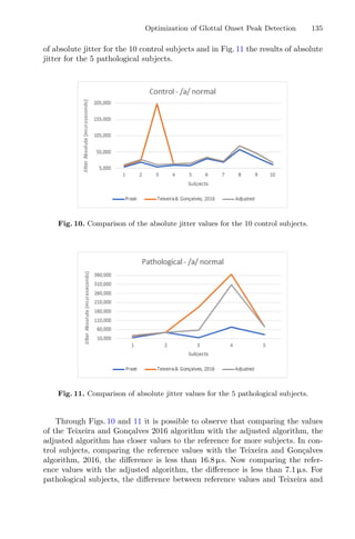
![Optimization of Glottal Onset Peak Detection 137
6. Kadiri, S., Alku, P.: Analysis and detection of pathological voice using glottal
source features. IEEE J. Sel. Top. Signal Process. 14(2), 367–379 (2020)
7. Teixeira, J.P., Teixeira, F., Fernandes, J., Fernandes, P.O.: Acoustic analysis of
chronic laryngitis - statistical analysis of sustained speech parameters. In: 11th
International Conference on Bio-Inspired Systems and Signal Processing, BIOSIG-
NALS 2018, vol. 4, pp. 168–175 (2018)
8. Sripriya, N., Poornima, S., Shivaranjani, R., Thangaraju, P.: Non-intrusive tech-
nique for pathological voice classification using jitter and shimmer. In: International
Conference on Computer, Communication and Signal Processing (ICCCSP), pp.
1–6 (2017)
9. Teixeira, J.P., Fernandes, P.: Acoustic analysis of vocal dysphonia. Procedia Com-
put. Sci. 64, 466–473 (2015)
10. Teixeira, J.P., Gonçalves, A.: Accuracy of jitter and shimmer measurements. Pro-
cedia Technol. 16, 1190–1199 (2014)
11. Teixeira, J.P., Gonçalves, A.: Algorithm for jitter and shimmer measurement in
pathologic voices. Procedia Comput. Sci. 100, 271–279 (2016)
12. Boersma, P., Weenink, D.: Praat: doing phonetics by computer [Computer pro-
gram]. Version 6.0.48, 15 April 2019 (1992–2019). http://www.praat.org/
13. Barry, W., Pützer, M.: Saarbruecken Voice Database. Institute of Phonetics at the
University of Saarland (2007). http://www.stimmdatenbank.coli.uni-saarland.de.
Accessed 15 Apr 2021](https://image.slidesharecdn.com/optimizationlearningalgorithmsandapplications-231204021346-9e8015c0/85/Optimization-Learning-Algorithms-and-Applications-pdf-150-320.jpg)
![Searching the Optimal Parameters
of a 3D Scanner Through Particle
Swarm Optimization
João Braun1,2(B)
, José Lima2,3
, Ana I. Pereira2
, Cláudia Rocha3
,
and Paulo Costa1,3
1
Faculty of Engineering, University of Porto, Porto, Portugal
paco@fe.up.pt
2
Research Centre in Digitalization and Intelligent Robotics,
Instituto Politécnico de Bragança, Bragança, Portugal
{jbneto,jllima,apereira}@ipb.pt
3
INESC-TEC - INESC Technology and Science, Porto, Portugal
claudia.d.rocha@inesctec.pt
Abstract. The recent growth in the use of 3D printers by independent
users has contributed to a rise in interest in 3D scanners. Current 3D
scanning solutions are commonly expensive due to the inherent complex-
ity of the process. A previously proposed low-cost scanner disregarded
uncertainties intrinsic to the system, associated with the measurements,
such as angles and offsets. This work considers an approach to estimate
these optimal values that minimize the error during the acquisition. The
Particle Swarm Optimization algorithm was used to obtain the param-
eters to optimally fit the final point cloud to the surfaces. Three tests
were performed where the Particle Swarm Optimization successfully con-
verged to zero, generating the optimal parameters, validating the pro-
posed methodology.
Keywords: Nonlinear optimization · Particle swam optimization · 3D
scan · IR sensor
1 Introduction
The demand for 3D scans of small objects has increased over the last few years
due to the availability of 3D printers for regular users. However, the solutions are
usually expensive due to the complexity of the process, especially for sporadic
users. There are several approaches to 3D scanning, with the application, in
general, dictating the scanning system’s requirements. Thus, each of them can
differ concerning different traits such as acquisition technology, the structure
of the system, range of operation, cost, and accuracy. In a more general way,
these systems can be classified as contact or non-contact, even though there are
several sub-classifications inside these two categories, which the reader can find
with more detail in [2].
c
Springer Nature Switzerland AG 2021
A. I. Pereira et al. (Eds.): OL2A 2021, CCIS 1488, pp. 138–152, 2021.
https://doi.org/10.1007/978-3-030-91885-9_11](https://image.slidesharecdn.com/optimizationlearningalgorithmsandapplications-231204021346-9e8015c0/85/Optimization-Learning-Algorithms-and-Applications-pdf-151-320.jpg)
![Optimal Parameters of a 3D Scanner Through PSO 139
Two common approaches for reflective-optical scanning systems are triangu-
lation and time-of-flight (ToF). According to [6], the range and depth variation
in triangulation systems are limited, however, they have greater precision. In
contrast, ToF systems have a large range and depth variation at the cost of
decreased precision. The triangulation approach works, basically, by projecting
a light/laser beam over the object and capturing the reflected wave with a digi-
tal camera. After that, the distance between the object and the scanning system
can be computed with trigonometry, as the distance between the camera and
the scanning system is known [6]. On the other hand, the accuracy of ToF-
based systems is mainly determined by the sensor’s ability to precisely measure
the round-trip time of a pulse of light. In other words, by emitting a pulse of
light and measuring the time that the reflected light takes to reach the sensor’s
detector, the distance between the sensor and the object is measured. Besides,
still regarding ToF-based systems, there is another approach to measure the
distance between the sensor and the object based on the Phase-Shift Method,
which essentially compares the phase shift between the emitted and reflected
electromagnetic waves.
Each approach has its trade-offs, which a common one is between speed and
accuracy in these types of scanning systems. By increasing the scanning speed of
the system, the accuracy will decrease, and vice-versa. This is mitigated by hav-
ing expensive rangefinders with higher sampling frequencies. In addition, accu-
racy during acquisition can be heavily affected by light interference, noise, and
the angle of incidence of the projected beam in the object being much oblique.
Therefore, a controlled environment, and a high-quality sensor and circuit must
be used to perform quality scans. However, the angle of incidence is less con-
trollable since it depends on the scanning system and the object (trade-off of
the system’s structure). In general, these types of 3D scanning systems are very
expensive, especially when even the cheaper ones are considered costly by the
regular user. A particular example includes a low-cost imagery-based 3D scanner
for big objects [18].
A low-cost 3D scanning system that uses a triangulation approach with an
infra-red distance sensor targeting small objects, therefore having limited range
and requiring large accuracy, was proposed and validated both in simulation [5]
and real scenarios, where the advantages and disadvantages of this architecture
were also addressed. Although the proposed system already has good accuracy,
it is possible to make some improvements with a multivariable optimization app-
roach. This is possible because the system makes some assumptions to perform
the scan that, although are true in simulation, do not necessarily hold in a real
scenario. One example is the object not being exactly centered on the scanning
platform. The assumptions, as well as the problem definition, are described in
Subsect. 4.1. The reasons why PSO was chosen instead of other approaches are
addressed in Subsect. 4.2.
The paper is structured as follows: a brief state of the art is presented in Sect. 2.
Section 3 describes the 3D scanning system and how it works. The optimization
problem is defined, and a solution is proposed in Sect. 4. The results are described
in Sect. 5. Finally, the last section presents the conclusion and future works.](https://image.slidesharecdn.com/optimizationlearningalgorithmsandapplications-231204021346-9e8015c0/85/Optimization-Learning-Algorithms-and-Applications-pdf-152-320.jpg)
![140 J. Braun et al.
2 State of the Art
As the field of optimization is vast, there are works in several fields of knowledge.
Therefore, in this section, the objective is to give a brief literature review on
multivariable optimization. Thus, some recent examples follow below.
Regarding optimization for shape fitting, [9] proposed a 3D finite-element
(FE) modeling approach to obtain models that represent the shape of grains
adaptively. According to the authors, the results show that the proposed app-
roach supports the adaptive FE modeling for aggregates with controllable accu-
racy, quality, and quantity, which indicates reliable and efficient results. More-
over, authors in [11], proposed an approach that combined an optimization-
based method with a regression-based method to get the advantages of both
approaches. According to the authors, model-based human pose estimation is
solved by either of these methods, where the first leads to accurate results but is
slow and sensitive to parameter initialization, and the second is fast but not as
accurate as of the first, requiring huge amounts of supervision. Therefore, they
demonstrated the effectiveness of their approach in different settings in compar-
ison to other state-of-the-art model-based pose human estimation approaches.
Also, a global optimization framework for 3D shape reconstruction from sparse
noisy 3D measurements, that usually happens in range scanning, sparse feature-
based stereo, and shape-from-X, was proposed in [13]. Their results showed that
their approach is robust to noise, outliers, missing parts, and varying sampling
density for sparse or incomplete 3D data from laser scanning and passive multi-
view stereo.
In addition, there are several works in multivariable optimization for mechan-
ical systems. For instance, the characteristics, static and dynamic, of hydrostatic
bearings were improved with controllers that were designed for the system with
the help of a multivariable optimization approach for parameter tuning [16]. The
authors proposed a control approach that has two inputs, a PID (Proportional
Integral Derivative) sliding mode control and feed-forward control, where the
parameters of the first input, were optimized with Particle Swarm Optimization
(PSO). Their results performed better compared with results from the literature
which had PID control. In addition, a system that consists of multi-objective
particle swarm optimized neural networks (MOPSONNS) was proposed in [8]
to compute the optimal cutting conditions of 7075 aluminum alloys. The sys-
tem uses multi-objective PSO and neural networks to determine the machining
variables. The authors concluded that MOPSONNS is an excellent optimization
system for metal cutting operations where it can be used for other difficult-
to-machine materials. The authors in [20] proposed a multi-variable Extremum
Seeking Control as a model-free real-time optimizing control approach for oper-
ation of cascade air source heat pump. They used for the scenarios of power
minimization and coefficient of performance maximization. Their approach was
validated through simulation which their results showed good convergence per-
formance for both steady-state and transient characteristics. The authors in
[7] applied two algorithms, continuous ant colony algorithm (CACA) and mul-
tivariable regression, to calculate optimized values in back analysis of several](https://image.slidesharecdn.com/optimizationlearningalgorithmsandapplications-231204021346-9e8015c0/85/Optimization-Learning-Algorithms-and-Applications-pdf-153-320.jpg)
![Optimal Parameters of a 3D Scanner Through PSO 141
geomechanical parameters in an underground hydroelectric power plant cavern.
The authors found that the CACA algorithm showed better performance. To
improve the thermal efficiency of a parabolic trough collector, authors in [1]
presented a multivariate inverse artificial neural network (ANNim) to determine
several optimal input variables. The objective function was solved using two
meta-heuristic algorithms which are Genetic Algorithm (GA) and PSO. The
authors found that although ANNim-GA runs faster, ANNim-PSO has better
precision. The authors stated that the two presented models have the potential
to be used in intelligent systems.
Finally, there are optimization approaches in other areas such as control the-
ory, chemistry, and telecommunication areas. Here are some examples. In control
theory, by employing online optimization, a filtering adaptive tracking control
for multivariable nonlinear systems subject to constraints was proposed in [15].
The proposed control system maintains tracking mode if the constraints are not
violated, if not, it switches to constraint violation avoidance control mode by
solving an online constrained optimization problem. The author showed that
the switching logic avoids the constraints violation at the cost of tracking per-
formance. In chemistry, artificial neural networks were trained under 5 different
learning algorithms to evaluate the influence of several input variables to pre-
dict the specific surface area of synthesized nanocrystalline NiO-ICG composites,
where the model trained with the Levenberg-Marquardt algorithm was chosen
as the optimum algorithm for having the lowest root means square error [17].
It was found that the most influential variable was the calcination temperature.
At last, in telecommunications, Circular Antenna Array synthesis with novel
metaheuristic methods, namely Social Group Optimization Algorithm (SGOA)
and Modified SGOA (MSGOA), was presented in [19]. The authors performed
a comparative study to assess the performance of several synthesis techniques,
where SGOA and MGSOA had good results.
As there aren’t any related works similar to our approach, the contribution of
this work is to propose a procedure to find the optimal parameters (deviations)
of a 3D scanner system through PSO, guaranteeing a good fit for point clouds
over their respective scanned objects.
3 3D Scanning System
The scanning system works basically in two steps. First, the object is scanned
and the data, in spherical coordinates, is saved in a point cloud file. After this,
a software program performs the necessary transformations to cartesian coordi-
nates and generates STL files that correspond to the point clouds. The flowchart
of the overall STL file generation process is presented in Fig. 1a. A prototype
of the low-cost 3D scanner, illustrated in Fig. 1b, was developed to validate the
simulated concept in small objects [5].
The architecture regarding the components and the respective communica-
tion protocols of the 3D scanning system can be seen in Fig. 2.](https://image.slidesharecdn.com/optimizationlearningalgorithmsandapplications-231204021346-9e8015c0/85/Optimization-Learning-Algorithms-and-Applications-pdf-154-320.jpg)
![Optimal Parameters of a 3D Scanner Through PSO 143
The dynamics of the 3D scanner is illustrated throughout a flowchart, which
can be seen in Fig. 3. The rotating structure keeps rotating until it finishes one
cycle of 360◦
. After this, the system increments the sensor’s angle by 2◦
. This
dynamic keeps repeating until the sensor’s angle reaches 90◦
. Afterward, the
data, in spherical coordinates, is saved to a point cloud file. The data conversion
to Cartesian coordinates is explained in detail in Sect. 4. The algorithm that
generates the STL files is outside of the scope of this work, for further information
the reader is referred to [5].
Fig. 3. 3D scanner dynamics flowchart.
4 Methodology
The notation used in this work to explain the system considers spherical coordi-
nates, (l, θ, ϕ). The scanning process starts by placing the object on the center
of the rotating plate (P = (0, 0, hp)), which is directly above the global reference
frame. The system is represented in Fig. 4, from an XZ plane view. First, the
slope’s angle measured from the X axis to the Z axis, with range [0, π/2] rad, is
θ. Also, ϕ is the signed azimuthal angle measured from the X axis, in the XY
plane, with range [0, 2π]. The parameter hp represents the distance from the
rotating plate to the arm rotation point, and hs is the perpendicular distance
from the arm to the sensor. The parameter l defines the length of the mechanical
arm and d represents the distance from the sensor to the boundary of the object
which is located on the rotating plate.
The position of the sensor s (red circle of Fig. 4) Xs = (xs, ys, zs), in terms of
the parameters (l, θ, ϕ), can be defined as follows, assuming the reference origin
at the center of the rotating base:
⎧
⎨
⎩
xs = (l cos(θ) − hs sin(θ)) cos(ϕ)
ys = (l cos(θ) − hs sin(θ)) sin(ϕ)
zs = l sin(θ) + hs cos(θ) − hp
(1)
Therefore, Xp = (xp, yp, zp), which is the position of a scanned point in a
given time in relation to the rotating plate reference frame, is represented by a
translation considering ||Xs|| and d. Thus, it is possible to calculate Xp as:](https://image.slidesharecdn.com/optimizationlearningalgorithmsandapplications-231204021346-9e8015c0/85/Optimization-Learning-Algorithms-and-Applications-pdf-156-320.jpg)
![146 J. Braun et al.
class of algorithms inspired by natural social intelligent behaviors. Developed
by Kennedy and Eberhart (1995) [10], this method consists on finding the solu-
tion through the exchange of information between individuals (particles) that
belong to a swarm. The PSO is based on a set of operations that promote the
movements of each particle to promising regions in the search space [3,4,10].
This approach was chosen because it has several advantages, according to
[12], such as:
– Easy in concept and implementation in comparison to other approaches.
– Less sensitive to the nature of the objective function regarding to other meth-
ods.
– Has limited number of hyperparameters in relation to other optimization
techniques.
– Less dependent of initial parameters, i.e., convergence from algorithm is
robust.
– Fast calculation speed and stable convergence characteristics with high-
quality solutions.
However, every approach has its limitations and disadvantages. For instance,
authors in [14] stated that one of the disadvantages of PSO is that the algorithm
easily fall into local optimum in high-dimensional space, and therefore, have a
low convergence rate in the iterative process. Nevertheless, the approach showed
good results for our system.
5 Results
To test the approach three case objects were analyzed: Centered sphere, Sphere
and Cylinder.
The first and second case were spheres with radius of 0.05 m. The first sphere
was centered on the rotating plate where the other had an offset of X,Y =
[0.045, 0.045]m. Finally, the third object was a cylinder with h = 0.08 m and
r = 0.06 m.
Since PSO is a stochastic method, 20 independent runs were done to obtain
more reliable results. The Table 1 presents the results obtained by PSO, describ-
ing the best minimum value obtained on the executed runs, the minimum average
from all runs (Av) and their respective standard deviation (SD). To analyze the
behavior of the PSO method, the results considering all runs (100%) and 90%
of best runs are also presented.
First, the results were very consistent for all the cases as can be verified by
the standard deviations, average values, and minima being practically zero. This
is also corroborated by comparing the results from all runs (100%) with 90% of
the best runs, where the averages from (100%) matched the averages from (90%)
of best runs and the standard deviations values maintained the same order of
magnitude. Also, another way to look at the consistency is by comparing the best
minimum value of executed runs with their respective averages, where all cases
match. Still, the only case where the PSO algorithm suffered a little was the](https://image.slidesharecdn.com/optimizationlearningalgorithmsandapplications-231204021346-9e8015c0/85/Optimization-Learning-Algorithms-and-Applications-pdf-159-320.jpg)
![Optimal Parameters of a 3D Scanner Through PSO 147
Table 1. PSO results for the three objects
Minimum 100% 90%
Av SD Av SD
Centered Sphere 7.117 × 10⁻⁸ 7.117 × 10⁻⁸ 5.8 × 10⁻¹⁴ 7.117 × 10⁻⁸ 6.06 × 10⁻¹⁴
Sphere 4.039 × 10⁻⁵ 4.039 × 10⁻⁵ 1.3 × 10⁻¹³ 4.039 × 10⁻⁵ 1.18 × 10⁻¹³
Cylinder 3.325 × 10⁻² 3.325 × 10⁻² 3.2 × 10⁻⁷ 3.325 × 10⁻² 2.4 × 10⁻⁷
cylinder, where although the minimum tended to 0, it didn’t reached the same
order of magnitude of the other cases. Therefore, we can confirm that the PSO
achieved global optimum in the sphere cases, on the other hand, the cylinder
case is dubious. There is also the possibility that the objective function for the
cylinder case needs some improvements.
In terms of minimizers, they are described in Table 2. It is possible to see that
for the centered sphere, all the parameters are practically 0. This is expected,
since the centered sphere did not have any offsets. The same can be said for the
cylinder. Finally, for the sphere, it is possible to see that although the sphere
had offsets of X, Y = [0.045, 0.045], the minimizers of X, Y are pratically zero.
This is also expected since as the sphere was displaced on the rotating plate, the
sensor acquired data points from the plate itself (on the center). Therefore, the
portion of the points representing the sphere was already ”displaced” during the
acquisition, i.e., the offsets in X, Y were already accounted for during acquisition.
By consequence, during transformation to cartesian coordinates. Therefore, the
only offset that was impactful on the transformation was the ϕoffset minimizer,
where it accounts for a rotation in the Z axis (to rotate the point cloud to
match the object). Of course, the other minimizers had their impact as well
during transformation.
Table 2. Minimizers obtained by PSO
xoffset[m] yoffset[m] ϕoffset[rad] θoffset[rad] γoffset[rad]
Centered Sphere −4.704 × 10⁻⁷
−5.472 × 10⁻⁸
−5.031 × 10⁻⁶
+4.953 × 10⁻⁵
+2.175 × 10⁻⁵
Sphere −7.579 × 10⁻³
8.087 × 10⁻²
1.566 × 10⁻¹
−8.885 × 10⁻⁵
−1.661 × 10⁻⁴
Cylinder 5.055 × 10⁻⁴
−3.371 × 10⁻⁴
−2.862 × 10⁻¹
5.046 × 10⁻²
1.057 × 10⁻¹
The behavior of the PSO approach for the centered sphere, its representation
in simulation, and its optimized point cloud over the original object can be seen,
respectively, in Figs. 6, 7a, and 7b.
As can be seen from the illustrations, and from Tables 1 and 2, the PSO
managed to find the global optimum of the system’s parameters. Note that,
in Fig. 6, the algorithm converged to the global minimum near iteration 15,
nevertheless it ran for more than 70 iterations (note that these iterations are
from the PSO algorithm itself, therefore they belong to just one run from the all](https://image.slidesharecdn.com/optimizationlearningalgorithmsandapplications-231204021346-9e8015c0/85/Optimization-Learning-Algorithms-and-Applications-pdf-160-320.jpg)
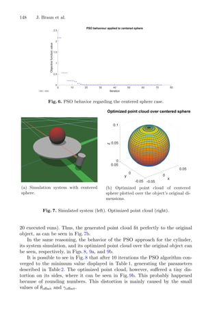
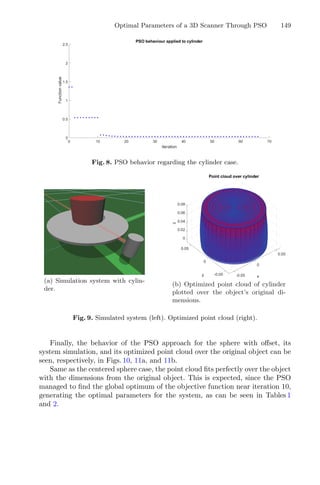
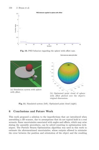


![Optimal Sizing of a Hybrid Energy
System Based on Renewable Energy
Using Evolutionary Optimization
Algorithms
Yahia Amoura1(B)
, Ângela P. Ferreira1
, José Lima1,3
,
and Ana I. Pereira1,2
1
Research Centre in Digitalization and Intelligent Robotics (CeDRI),
Instituto Politécnico de Bragança, Bragança, Portugal
{yahia,apf,jllima,apereira}@ipb.pt
2
Algoritmi Center, University of Minho, Braga, Portugal
3
INESC-TEC - INESC Technology and Science, Porto, Portugal
Abstract. The current trend in energy sustainability and the energy
growing demand have given emergence to distributed hybrid energy sys-
tems based on renewable energy sources. This study proposes a strategy
for the optimal sizing of an autonomous hybrid energy system integrat-
ing a photovoltaic park, a wind energy conversion, a diesel group, and
a storage system. The problem is formulated as a uni-objective func-
tion subjected to economical and technical constraints, combined with
evolutionary approaches mainly particle swarm optimization algorithm
and genetic algorithm to determine the number of installation elements
for a reduced system cost. The computational results have revealed an
optimal configuration for the hybrid energy system.
Keywords: Renewable energy · Hybrid energy system · Optimal
sizing · Particle swarm optimisation · Genetic algorithm
1 Introduction
The depletion of fossil resources, impacts of global warming and the global aware-
ness of energy-related issues have led in recent years to a regain of interest in
Renewable Energy Sources (RES), these latter benefit from several advantages
which enable them to be a key for the major energy problems. On the other hand,
a remarkable part of the world’s population does not have access to electricity
(approximately 13% of the population worldwide in 2016) [1], which creates an
important limitation for their development. Nevertheless, these needs can be
covered by a distributed generation provided by renewable energy systems with
the implementation of insulated microgrids based on Hybrid Energy Systems
(HES) offer a potential solution for sustainable, energy-efficient power supply,
providing a solution for increasing load growth and they are a viable solution to
c
Springer Nature Switzerland AG 2021
A. I. Pereira et al. (Eds.): OL2A 2021, CCIS 1488, pp. 153–168, 2021.
https://doi.org/10.1007/978-3-030-91885-9_12](https://image.slidesharecdn.com/optimizationlearningalgorithmsandapplications-231204021346-9e8015c0/85/Optimization-Learning-Algorithms-and-Applications-pdf-166-320.jpg)
![154 Y. Amoura et al.
the electrification of remote areas. These microgrids can be exploited connected
to the main grid, with the latter acting as an energy buffer, or in islanded mode.
One of the most important benefits of the RES remains in their contribution to
the solution of global warming problems by avoiding damaging effects such as
greenhouse gas emissions (GHG), stratospheric ozone hole, etc.
Despite technological advances and global development, renewable energy
sources do not represent a universal solution for all current electricity supply
problems. There are several reasons for this, for instance, the low efficiency
compared to conventional sources. Economically, RES provides extra costs and
their payback takes a longer period [2]. In addition, RES are in a large extent,
unpredictable and intermittent due to the stochastic nature of, for instance,
solar and wind sources. To overcome the mismatch between the demand and
the availability of renewable energy sources, typically microgrids are based on
the hybridization of two or more sources and/or the exploitation of storage
systems [3]. By this way, the complementarity between different renewable energy
sources, together with dispatchable conventional sources, gives the emergence of
hybrid energy systems (HES) which represent an ideal solution for the indicated
problems.
Under the proposed concept of HES, in the event that renewable energy
production exceeds the demand, the energy surplus is stored in system devices
as chemical ones or hydrogen-based storage systems, or, in alternative, delivered
to the grid [4].
To increase the interest and improve the reliability of hybrid energy systems,
it is important to provide new solutions and address an essential problem con-
sisting of their optimal sizing. To deal with this type of problem, researchers have
often referred to optimization methods. For instance, in [5] researchers have used
the Sequential Quadratic Programming (SQP) method. Navid et al. [6] have used
the Mixed Integer Non-Linear Programming (MINLP) method, the stochastic
discrete dynamic programming has been used on [7]. Kusakana et al. [8] have
developed an optimal sizing of a hybrid renewable energy plant using the Linear
Programming (LP) method. Among other approaches, in [9] metaheuristics have
proved to be an ideal optimization tool for the resolution of sizing problems.
The work presented in this paper presents a real case study addressing the
optimal sizing of a hybrid energy system in the campus of Santa Apolónia located
in Bragança, Portugal. The objective of the work is to determine the optimal
number of renewable energy-based units: photovoltaic modules and wind con-
version devices on the one hand, and the optimal number of batteries for storage
on the other hand. The contribution of this article consists in the development
of an optimal sizing software based on optimization approaches. Because of the
stochastic effect of the problem that represents a random effect especially in
terms of power produced by the renewable energies sources, it is proposed to
deal with the optimization problem using metaheuristic algorithms, mainly, Par-
ticle Swarm Optimisation (PSO) algorithm and Genetic algorithm (GA). The
PSO is a modern heuristic search approach focused on the principle of swarm-
ing and collective behavior in biological populations. PSO and GA belong to](https://image.slidesharecdn.com/optimizationlearningalgorithmsandapplications-231204021346-9e8015c0/85/Optimization-Learning-Algorithms-and-Applications-pdf-167-320.jpg)
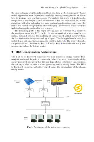

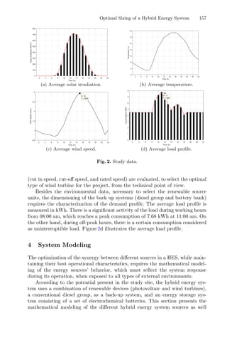
![158 Y. Amoura et al.
as the characteristics of the device units adopted, taking into consideration the
environmental data collected and presented in the previous section.
4.1 Photovoltaic Energy System
Considering the objectives of this work, the most suited model for the photo-
voltaic energy system conversion is the power model (input/output) [10], which
has the advantage of estimating the energy produced by the photovoltaic appara-
tus from the global irradiation data and the ambient temperature on an inclined
plane, as well as the manufacturer’s data for the photovoltaic module selected.
The power output of a photovoltaic module can be calculated according to
the following equation:
Ppv(t) = ηSG (1)
being η the instantaneous efficiency of the photovoltaic module, S the surface of
the photovoltaic module and G the global irradiation on an inclined plane.
The instantaneous efficiency is given by,
η = ηr(1 − γ(Tc − T0)) (2)
where ηr is the reference efficiency of the photovoltaic module under standard
conditions (T0 = 25◦
C, G0 = 1000 W/m
2
and AM = 1.5), γ is the temperature
coefficient (◦
C) determined experimentally as the variation in module efficiency
for a 1◦
C variation in cell temperature (it varies between 0.004 and 0.006◦
C), Tc
is the temperature of the module that varies with the irradiance and the ambient
temperature as follows:
Tc = Ta +
NOCT − 20
800
G (3)
being NOCT the nominal operating cell temperature and Ta the ambient tem-
perature in (◦
C).
Thus, the instantaneous total power of the photovoltaic array, Pt
pv, is written
as follows:
Pt
pv(t) = Ppv(t)Npv (4)
where Npv is the number of modules to be used in the photovoltaic array.
The main characteristics of the selected photovoltaic module are presented
in [11].
4.2 Wind Energy Conversion System
The power produced by a wind energy system at a given site depends on the
wind speed at a hub height, the air density, and the specific characteristics of
the turbine. The wind speed in (m/s) at any hub height can be estimated using
the following law:](https://image.slidesharecdn.com/optimizationlearningalgorithmsandapplications-231204021346-9e8015c0/85/Optimization-Learning-Algorithms-and-Applications-pdf-171-320.jpg)
![Optimal Sizing of a Hybrid Energy System 159
v = vi
h
hi
λ
(5)
being hi the height of the measurement point, generally taken at 10 m, vi is the
speed measured at height hi (m/s) and λ is typically taken as 1/7.
The modeling of the power produced by a wind energy system unit Pwt is
selected as a linear model [12], as follows:
⎧
⎪
⎪
⎨
⎪
⎪
⎩
Pwt = 0, v ≥ vc, v vd
Pwt = Pn
v − vd
vn − vd
, vd ≤ v vn
Pwt = Pn, vn ≤ v vc
(6)
where Pn is the rated electrical power of the wind turbine unit, v is the value of
the wind speed, vn is the rated speed of the wind turbine, vc is the cut-off speed
and vd is the cut-in speed of the wind turbine.
The instantaneous total power produced by a wind farm, Pt
wt, is given by
the number of wind energy units, Nwt, times the power of each unit, as follows:
Pt
wt(t) = Pwt(t)Nwt (7)
The features of the selected module of the wind energy conversion system are
presented in [13].
4.3 Energy Storage System
The modeling of the energy storage system (ESS) is divided into two steps
according to two operations. The first step consists of evaluating the total capac-
ity of the battery bank for an autonomy duration determined by the required
specifications. By this way it will be possible to determine the unit capacity of
a battery unit and therefore the number of batteries for the required autonomy,
without the intervention of other production sources. The second step will be
the study of the batteries’ behavior in the chosen sizing configuration to assess
the feasibility of the first step. Therefore, it will be possible to know the exact
number of batteries that will be operating in parallel with the other production
sources, mainly the photovoltaic and wind turbine systems, without any system
interruption.
Sizing the Capacity of the Battery Bank. The total rated capacity of the
batteries, C, should satisfy the following formulation:
C =
NjEneed
PdKt
(8)
being Nj the required autonomy in days, Eneed the daily energy, Pd the allowed
depth of discharge and Kt the temperature coefficient of the capacity.](https://image.slidesharecdn.com/optimizationlearningalgorithmsandapplications-231204021346-9e8015c0/85/Optimization-Learning-Algorithms-and-Applications-pdf-172-320.jpg)
![160 Y. Amoura et al.
Battery Energy Modelling. The battery energy modeling establishes an opti-
mal energy storage management. This operation depends on the previous state
of charge and the differential between the energy produced by the different types
of generators, Epr, and the initial energy required by the load, Ed defined by:
Ed(t) = Et
load(t) − (Epr(t)) (9)
where,
Epr(t) = Et
pv(t) + Et
wt(t) (10)
and ⎧
⎨
⎩
Et
pv(t) = Pt
pv(t)Δt
Et
wt(t) = Pt
wt(t)Δt
Et
load(t) = Pt
load(t)Δt
(11)
knowing that Δt is the simulation step, defined as one-hour interval.
Batteries state of charge can be evaluated according to two operation modes,
described as follows.
• Charging operating mode: If Epr ≥ Ed. The instantaneous energy storage
capacity, E(t), is given by the following equation:
E(t) = E(t − 1) + ηbat
Epr(t)ηconv −
Ed(t)
ηconv
(12)
being ηbat the battery efficiency and ηconv the converter efficiency.
• Discharging operating mode: If Epr Ed. Now, the instantaneous storage
energy capacity can be expressed as follows:
E(t) = E(t − 1) +
1
ηbat
(Epr(t)ηconv − Ed(t)) (13)
The instantaneous state of the charge is given by:
SOC(t) =
E(t)
Etotal
(14)
In addition, the charging and discharging modes should guarantee that the state
of the charge (SOC) of the energy storage system must satisfy the following
condition:
SOCmin ≤ SOC(t) ≤ SOCmax (15)
being SOCmin and SOCmax the minimum and maximum state of charge of the
energy storage system respectively.
The specification of the proposed battery unit are described in [14].](https://image.slidesharecdn.com/optimizationlearningalgorithmsandapplications-231204021346-9e8015c0/85/Optimization-Learning-Algorithms-and-Applications-pdf-173-320.jpg)
![Optimal Sizing of a Hybrid Energy System 161
4.4 Diesel Generator
The rated power of the diesel generator, Pdg, is chosen equal to the maximum
power required by the load i.e.,
Pdg ≥ Pmax
load (t) (16)
The operating mode of the diesel group is based on two possible scenarios:
• The first scenario occurs when the power verifies the following relation:
Pt
pv(t) + Pt
wt(t) +
E(t)
Δt
≥ Pload(t) (17)
In this case, it is not necessary to start the generator as the consumption is
satisfied.
• The second scenario occurs when the following relationship is verified:
Pt
pv(t) + Pt
wt(t) +
E(t)
Δt
Pload(t) (18)
In this case, the generator starts up to cover all or part of the energy demand
in the absence of enough power from the other sources.
The technical specifications of the chosen diesel group are mentioned in [15].
5 Adopted Sizing Strategy
After performing load balance and evaluating the solar and wind potential pre-
sented earlier in Sect. 3, the renewable sources are designed to provide continuous
power to the required demand, then, taking into account the autonomy of the
load which is ensured by the storage system reaching 24 h. The latter will there-
fore be able to supply the energy necessary for the load without the presence of
other renewable sources for 24 h. The procedure to be followed is shown in the
flowchart by Fig. 3. First, the capacity of the battery bank is defined according
to the overall load and the desired autonomy, by using the Eq. (8) presented in
Sect. 4.3.
This step allows obtaining the necessary number of batteries, if there are
no renewable sources available, for a specific period of autonomy (24 h in this
case). The diesel generator is the last resource back up system, able to satisfy the
demand if there are no renewable energy available and the battery bank reaches
its minimum state of charge.
The intermittent nature of the renewables, makes the problem subject to
stochastic treatment. To solve the optimization problem, two metaheuristic
methods were used: Genetic Algorithm (GA) and Particle Swarm Optimisation
(PSO) algorithms. So, after providing the main initial data (meteorological data,
constraints and initial parameters) the values of the decisive variables obtained
by the algorithmic computation represent the optimal number of renewable gen-
erators. The algorithm evaluates them recursively until the cost of the installa-
tion is in the most optimal value.](https://image.slidesharecdn.com/optimizationlearningalgorithmsandapplications-231204021346-9e8015c0/85/Optimization-Learning-Algorithms-and-Applications-pdf-174-320.jpg)
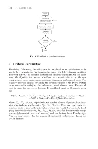
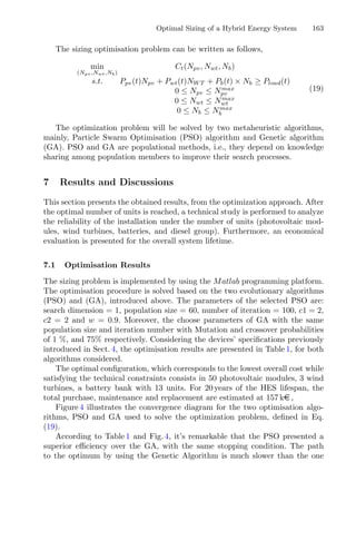
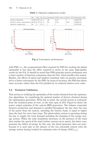
![Optimal Sizing of a Hybrid Energy System 165
To analyse the performance of the chosen diesel generator set in this micro-
grid, the system performance is analysed for 48 h, considering the hypothetical
scenario of null production of the renewable sources in the proposed time span.
According to Fig. 5b, the diesel generator is operational (working as back up
system) after the minimal state of charge of the energy storage system has been
reached, which justifies that the number Ndg = 1 is sufficient and optimal to
feed the installation in case of a supply absence.
(a) Presence of all sources. (b) Absence of renewable energies.
Fig. 5. Optimal power set-points describing the hybrid energy system behavior.
Figure 6a shows the evolution of the state of charge (SOC) of the battery
bank when operating in parallel with the other HES sources, for the time span
of 24 h. The energy of the batteries is used (discharged) mainly during the night
to supply the loads while the charging process is ensured during the day by the
surplus of the renewable sources, over the demand.
Figure 6b represents the capacity of the battery bank to maintain a 24-hour
autonomy adopting the Cycle Charge Strategy [16], while satisfying the needs
of the load, i.e. if the renewable sources (photovoltaic and wind systems) are
not available, the storage system will be able to provide the demand for 24 h,
without any interruption of the power supply.
The total discharge of the batteries contributes enormously to their life time
their life span reduction. For this reason, the SOC of the batteries should never
go below its minimum value. This constraint is thus verified since in this study
case the SOC of the energy storage system after 24 h of usage did not sink the
minimum state defined by 20% in the battery specification. Indeed, the number of
storage batteries delivered by the optimization algorithm computations discussed
above represents an optimal value.](https://image.slidesharecdn.com/optimizationlearningalgorithmsandapplications-231204021346-9e8015c0/85/Optimization-Learning-Algorithms-and-Applications-pdf-178-320.jpg)
![166 Y. Amoura et al.
(a) SOC of the battery bank in parallel
operation.
(b) SOC of the battery bank in autonomous
operation.
Fig. 6. Storage system behavior
7.3 Economical Evaluation
In order to evaluate the economic benefit of the overall installation, it is analysed
the profitability during its life cycle. The life time of the HES is 20 years, the
total purchase, maintenance and replacement costs are 157755.87 e . The average
power consumption during 24 h is 122.915 kWh, which is equivalent to a value
of 898508.65 kWh within 20 years, without taking into account the extension of
the load. Portugal has one of the most expensive electricity systems in Europe.
According with eurostat data in 2020, the price of electricity averaged 0.2159
e /kWh including taxes [17]. The estimated cost of the energy bill is 195964.74
e . These values allow to highlight the amount saved by the customer, as well
as the payback period.
Figure 7 shows an economic estimation for the life time under consideration.
The line in black shows the evolution of the energy bill according to conven-
tional energy from the public grid. The line in red represents the evolution of
the investment cost in the HES, this latter starts with an initial purchase cost
that increases each year with the amount of maintenance of the different ele-
ments, every 4 years the batteries are replaced without taking into account the
maintenance price of the batteries during the year of their replacement.
The intersection of the final value of the investment cost with the conventional
energy bill on the time axis represents the period when the customer recovers
the amount invested in the HES, and from that moment until the end of the
life of the HES all the money supposed to be spent on the energy bill of the
installation will be saved. It can be seen that the cost of the investment in the
HES will be repaid at the end of the 16th
year, more precisely on October 2037 if
it is considered that the system will be installed on 1 January 2021. In this case,
the HES is more profitable than conventional energy and allows the customer to
save a value of 35423.49 e .](https://image.slidesharecdn.com/optimizationlearningalgorithmsandapplications-231204021346-9e8015c0/85/Optimization-Learning-Algorithms-and-Applications-pdf-179-320.jpg)
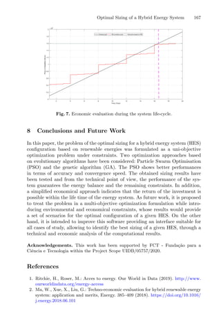


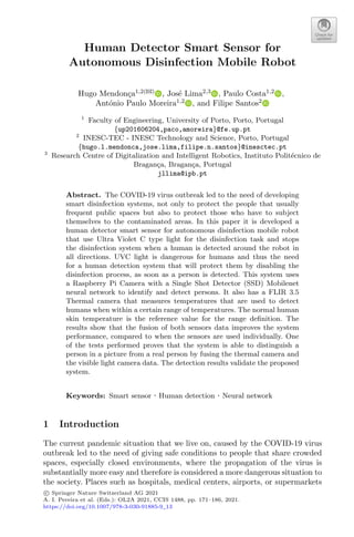
![172 H. Mendonça et al.
are among those that fit in the previous description and even though regular
testing to the users may be one way to prevent the spread of the virus, the
disinfection of public places is of great importance.
Disinfection using chemical products is one of the most popular but also
implies a lot of effort and risk by the user since they must submit themselves
to the dangerous conditions of proximity to possibly infected places. One way
to solve this problem is using an Automated Guided Vehicles (AGV) that can
cover large spaces without the supervision of human operators. Disinfection with
Ultraviolet Radiation is an alternative to the use of chemical products without
losing efficiency. This method works by exposing the infected area for a few
seconds to the UV radiation reducing the viral load that is present there.
This method is particularly interesting since it allows the disinfection of a
larger area in less time, and by using an AGV, this task can be programmed
to be performed during the periods without the presence of people (as example
airports and commercial areas). However, due to its danger for living organisms,
it is necessary to develop a system that detects persons that may be close to the
actuation zone.
This paper addresses a developed system that uses multiple sensors to have a
higher robustness of detecting humans without false positives and false negatives
by fusing the sensors signals that are captured individually in a single algorithm,
that will then communicate with the disinfection robot. False negatives have a
bigger impact in the system performance, since the disinfection lights are not
stopped when persons are near the robot. Results are very promising reaching
97% of accuracy.
The remaining of the paper is organized as follows. After an introduction
presented in Sect. 1, the Sect. 2 addresses the related work regarding the human
detection approaches. Then in Sect. 3, the system architecture is presented where
the thermal camera, the Raspberry pi camera and the LiDAR sensor to estimate
the disinfection time based on the room area are stressed. Section 4 presents the
results and its discussion. Finally, Sect. 5 presents the conclusions and points out
the future work directions.
2 Related Work
When trying to detect people in a closed environment, a multi-sensor approach
can be a good solution. Since it relies on the information of more than one sensor
to give a final, more accurate result, this method is the focus of this article. The
data gathered by the different cameras and other sensors are later fused and
analyzed allowing the system to have one single output. The system uses two
cameras, one visible light camera, and one thermal camera to run an active
detection algorithm. On the other hand, there are also two other sensor types, a
LiDAR that gives distance information on the direction where the cameras are
pointing and a Passive Infrared (PIR) sensor that is used in home surveillance
systems for motion detection [9,10,13]. This last type of sensor is also commonly
used to locate the motion target in space when using multiple sensors pointing](https://image.slidesharecdn.com/optimizationlearningalgorithmsandapplications-231204021346-9e8015c0/85/Optimization-Learning-Algorithms-and-Applications-pdf-184-320.jpg)
![Human Detector Smart Sensor for Autonomous Disinfection Mobile Robot 173
in different directions allowing the system to pinpoint to a certain degree its
position [5,15,17]. The most common LiDAR cannot distinguish what type of
objects are close to the system where is used, which means it cannot be used as
an active detection sensor. However the distance data can be used to allow the
system a better comprehension of what is happening around it by mapping the
environment [1] and working together with the cameras to improve the system
performance [4,12].
In regards to active human detection applications using cameras, thermal
cameras are a less indicative sensor of visual information since it only captures
temperatures based on infrared sensors. However in situations of low light, as
described in [3] and [16], this type of camera has more accurate detection results
when compared to visible light cameras without infrared sensors. In [7] a com-
parison is made between two cameras, one with and the other without infrared
modules and the first outperforms the second by far, thus making us believe that
in low light conditions thermal cameras are more informative than visible light
cameras.
Since some thermal cameras are usually expensive, it is necessary to find
one that meets our requirements but without compromising our budget. FLIR
Lepton represents such case as proven in [11] showing a capability to detect
specific temperatures of objects smaller than humans from long distances [3] in
a compact, low weight sensor compatible with embedded devices such as the
Raspberry Pi in our case. This model has two versions 2.x and 3.x where the
first has an 80 × 60 resolution and the second a 160 × 120 resolution among other
differences.
The visible light camera detection relies on previously trained models to
identify persons. This is commonly used in Internet of Things applications and
more complex surveillance systems [7], that instead or in addition to the use
of passive sensors such as PIR sensors also use computer vision and machine
learning to more accurately identify persons. Even though PIR sensors are a good
option in simple motion detection systems since they are cheap and easy to use.
Sometimes it triggers false positives which lead to unnecessary preoccupation and
false negatives when there is a person but it is not moving. The human detection
can be achieved by using image processing through background subtraction plus
face detection or head and shoulder detection [7], but also using machine learning
through networks prepared for the task of identification such as Convolutional
Neural Network (CNN) [14], DarkNET Deep Learning Neural Network [8] and
others such as YOLO and its variants, SSD and CNN variants [2].
3 System Architecture
The goal of this paper is to develop a human detection system that can be used
with an autonomous disinfection robot and it was developed to be a low-cost
and low weight efficient solution. The system will be mounted on top of a robot
equipped with a UVC light tower responsible for the disinfection procedure. The
human detector is a stand-alone equipment that is powered by 24 V and can](https://image.slidesharecdn.com/optimizationlearningalgorithmsandapplications-231204021346-9e8015c0/85/Optimization-Learning-Algorithms-and-Applications-pdf-185-320.jpg)
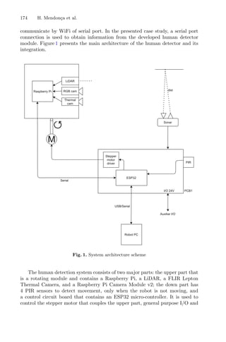

![176 H. Mendonça et al.
A range is set in the algorithm to consider a group of temperatures near
this ideal human temperature value considering two factors: human temperature
fluctuation and the camera precision of ±5 ◦
C. If the read value is situated
within this range we consider a positive human detection, even though we need
to consider other inputs, since there can be other objects in the range that have
the same temperature as the human body.
3.2 RGB Camera
The RGB camera used is a Raspberry Pi Camera Module v2 due to its low cost
and ease of use with the Raspberry Pi without compromising performance and
image quality.
The system uses a SSD Mobilenet model trained with COCO Dataset to
detect and identify persons in real-time through the Raspberry Pi camera.
The MobileNet was quantitized to a lower resolution (internal Neural Network
weights are moved from floats to integers), using the Tensorflow framework to
reduce the computational power requirement, and enable the use of this Neural
Network on a Raspberry Pi. As said in [6], a Single Shot multibox Detector (SSD)
is a rather different detection model from Region-CNN or Faster R-CNN. Instead
of generating the regions of interest and classifying the regions separately, SSD
does it simultaneously, in a “single-shot”.
SSD framework is designed to be independent of the base network, and so
it can run on top of other Convolutional Neural Networks (CNNs), including
Mobilenet.
The Mobilenet and Raspberry Pi are capable of detecting persons in the
chosen vertical resolution with a of 2,5 frames per second. In this case we defined
a threshold of 50% on MobileNet detection confidence to reduce the false positive
detections. The network is quite robust, having the capacity of detecting persons
in a different number of situations, like for example through a partial body image
or simply a single hand image.
3.3 LiDAR
The detection system also includes a LiDAR sensor pointing in the same direc-
tion as the cameras that are continuously sending to the Raspberry Pi distance
measurements. This information is useful for mapping applications recreating
the surrounding environment of the sensor giving yet another way of detection
to the system although is much less informative since it cannot distinguish dif-
ferent types of objects simply by using distance measurements. The disinfection
time can be tuned based on this information.
The used LiDAR is a TFMini Plus UART module, a low-cost, small-size,
and low power consumption solution to promoting cost-effective LiDARs. The
TFmini Plus LiDAR Modules emit modulation waves of near-infrared rays on a
periodic basis, which will be reflected after contacting the object. The time of
flight is then measured by the round-trip phase difference and then the relative
range is calculated between the product and the detection object.](https://image.slidesharecdn.com/optimizationlearningalgorithmsandapplications-231204021346-9e8015c0/85/Optimization-Learning-Algorithms-and-Applications-pdf-188-320.jpg)
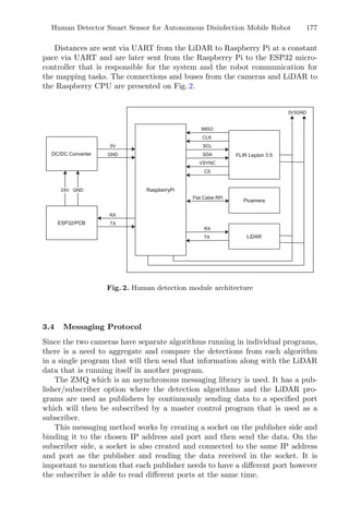
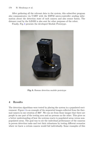
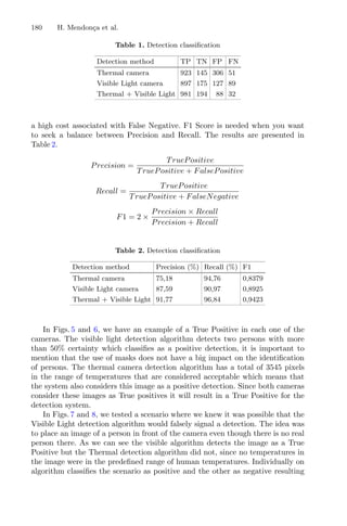
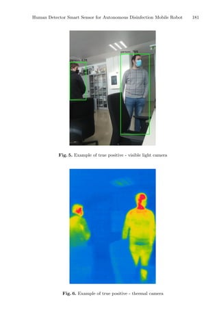


![188 D. Matos et al.
When the solution points out more than one AGV to transport the material,
a new problem must be tackled: scheduling of multiple AGV. The coordination
of a fleet of autonomous vehicles is a complex task and actually most available
multi-robot systems rely on static and pre-configured movements [1].
The solution can be composed by a cooperative movement between all robots
that are part of the system while avoiding mutual block. In fact, this problem
of scheduling for multiple-robots can be compared to the well-known problem of
the Travelling salesman problem applied with multiple salesman. However the
problem of task scheduling in multiple-robots system has the added complexity
that the path of one robot can interfere with the path of the other robots since
they all must share the same resources. Based on this, an optimisation method-
ology is proposed in this paper so that it can solve the multi-robot scheduling,
while taking into account the impact of the pathing conflicts in the overall effi-
ciency of the system. This paper addresses an optimisation approach based on
the estimation of the robots paths via the TEA* algorithm and the consequen-
tial optimisation of the scheduling of multiple AGV via the Simulated Annealing
algorithm.
1.1 Problem Description
The order in which the tasks are attributed to each of the agents of the system can
have a great impact in the overall efficiency of the system. Therefore, discovering
the ideal order of tasks to assign to each of the robots, that are part of a multi
AGV system, is a very important task.
The main goal of this article is to create a module that is capable of optimising
the task order that will be assigned to each of the robots. This optimisation
process must be time sensible, since it must generate a good solution in the time
interval that takes the control system of the multi AGV to execute its current
assigned tasks. This module uses a path estimation generated by the TEA* path
planning algorithm to calculate the cost of each solution taking into account the
possible resource conflicts.
Most task scheduling implementations do not take into account possible
pathing conflicts, that can occur during the planning of the paths for the
robots that comprise the system. These conflicts normally originate unpredicted
increases in the time it takes the system so execute the tasks, since in order to
solve these conflicts one more of the robots must either delay their movement or
use a less efficient path to reach the target. Therefore, the overall objective of this
optimisation is to make the system more efficient by using a path planning algo-
rithm in the optimisation phase. The path planning algorithm will generate an
estimation of the real paths of that the robots will take. The main idea behind
this system is to use this estimations to calculate the value of each solution,
therefore the minimisation of this value will be directly correlated to a decrease
in the number of pathing conflicts. In most real industrial applications of multi
AGV systems there are some restrictions associated with how the transport of
cargo can be made, for example some tasks can only be executed by certain
robots (due to the AGV characteristics) and some tasks have to be executed as](https://image.slidesharecdn.com/optimizationlearningalgorithmsandapplications-231204021346-9e8015c0/85/Optimization-Learning-Algorithms-and-Applications-pdf-200-320.jpg)
![Multiple Mobile Robots Scheduling Based on Simulated Annealing 189
soon as possible having priority over others, this restrictions were also taken into
account during the design of this module.
This article represents the first step into developing a system capable of such
optimisation. It presents the results of the study of the performance of one of the
most commonly used optimisation methods, when it is applied in the scenario
described above. This article also compares the performance of this method with
the results obtained from the minimisation of the travelled distance without
taking into consideration the path estimation. Since the purpose of this article is
just to study the performance of the Simulated Annealing algorithm when it is
apply to this case, the estimation of the AGV battery and the dynamic execution
of tasks were not taken into account, however such features are planned in future
iterations of this work.
For the purposes of this study a task is considered as the movement the
movement of the robot between two workstation. This implies that the robot
must first move from its current position towards the starting workstation, in
order to load the cargo, and then drop it at the final workstation. To execute
this movements the robot must access shared resources, due to the physical
dimensions of the robot and the operation space, it is considered that it is only
possible to have one robot travelling on each edge of the graph, in order to avoid
possible deadlock situations.
This types of studies are of paramount importance as a possible solution to
this optimisation problem may be based in a multi method based approach.
The paper is organised as follows. After this brief introduction, Sect. 2
presents some related work on the scheduling problem. Section 3 addresses the
system architecture whereas in Sect. 4 presents the optimisation methodology.
On Sect. 5, the results of the proposed method are stressed and Sect. 6 concludes
the paper and points out the future work direction.
2 State Art
Task scheduling defines and assigns the sequence of operations (while optimising)
to be done, in order to execute a set of tasks. Examples of scheduling can be
found in a huge number of processes, such as control air traffic control, airport
gate management, allocate plant and machinery resources and plan production
processes [2,4] among several others. The task scheduling can be applied to the
presented problem on assigning the task for each agent on a multi-robot system.
This problem can be considered a variant of the well known Travelling Salesman
Problem (TSP) [3].
According to [12], algorithms between centralised and decoupled planning
belong to three problem classes: 1) coordination along fixed, independent paths;
2) coordination along independent roadmaps; 3) general, unconstrained motion
planning for multiple robots. Following 3), there are several approaches to solve
the scheduling problems, from deterministic methods to heuristics procedures.
Regarding the Heuristic procedures there are several ways such as Artificial
Intelligence, Simulated Annealing (SA) and Evolutionary algorithms [5]. Classi-
cal optimisation methods can also be applied to the scheduling problem such as](https://image.slidesharecdn.com/optimizationlearningalgorithmsandapplications-231204021346-9e8015c0/85/Optimization-Learning-Algorithms-and-Applications-pdf-201-320.jpg)
![190 D. Matos et al.
the Genetic Algorithm (GA) or Tabu Search [6]. Enhanced Dijkstra algorithm
is applied to find the conflict-free routing task on the work proposed by [7].
The scheduling problem has been studied extensively in the literature. In
the robotics domain, when considering each robot as an agent, some of these
algorithms can be directly adapted. However, most of the existing algorithms
can only handle single-robot tasks, or multi-robot tasks that can be divided into
single-robot tasks. Authors from [8] propose an heuristics to address the multi-
robot task scheduling problem but at the coalition level, which hides the details
of robot specifications.
Scheduling problem can be solved resorting to several approaches, such as
mixed integer program, which is a standard approach in the scheduling com-
munity [15] or resorting to optimisation techniques: Hybrid Genetic Algorithm-
Particle Swarm Optimisation (HGA-PSO) multiple AGV [16], find the near-
optimum schedule for two AGVs based on the balanced workload and the min-
imum travelling time for maximum utilisation applying Genetic Algorithm and
Ant Colony Optimisation algorithm [14].
Other approaches provide a methodology for converting a set of robot trajec-
tories and supervision requests into a policy that guides the robots so that oper-
ators can oversee critical sections of robot plans without being over-allocated,
as an human-machine-interface proposal that indicates how to decide the re-
planning [9]. Optimisation models can also help operators on scheduling [10].
Similar approach is stressed on [11] where the operator scheduling strategies
are used in supervisory control of multiple UAVs. Scheduling for heterogeneous
robots can also be found on literature but addressing two agents only [13].
Although there exist some algorithms that support complex cases, they do not
represent efficient and optimised solutions that can be adapted for several (more
than two) multi-robot systems in a convenient manner. This paper proposes a
methodology, based on Simulated Annealing optimisation algorithm, to schedule
a fleet of four and eight robots having in mind the simultaneous reduction of
the distance travelled by the robots and the time it takes to accomplish all the
assigned tasks.
3 System Architecture
The system used to test the performance of the optimisation methods, as shown
in Fig. 1, is comprised of two modules:
– The Optimisation module;
– The Path Estimation module;
The idea behind this study is to, at a later date, use its results to help design
and implement a tasks scheduling software that will work as an interface between
the ERP used for industrial management and the Multi AGV Control System.
The Optimisation module will use the implemented methodologies, described
in Sect. 4, to generate optimised sets of tasks for each of the robots. These sets are
then sent to the Path Estimation module, this module estimates the paths that](https://image.slidesharecdn.com/optimizationlearningalgorithmsandapplications-231204021346-9e8015c0/85/Optimization-Learning-Algorithms-and-Applications-pdf-202-320.jpg)
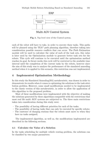
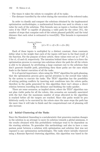
![Multiple Mobile Robots Scheduling Based on Simulated Annealing 193
algorithm presented by [17,18] to solve the traditional Multiple Travelling Sales-
man Problem (mTSP).
This initial clustering uses a matrix with the distance between the final point
of each task and the beginning point of the other tasks, in order to create a
number of clusters equal to the number of robots available in the system. Due
to the fact that the beginning point and final point of each task are usually
different, the distance matrix computed is not symmetric. This asymmetry serves
to model the fact that the order in which the tasks are executed by each robot
is not commutative and does have a large impact in the value of the solution.
These clusters were then assigned to the robot that was closest to the start
point of each cluster. This solution will serve as the baseline for the optimisation
executed by the Simulated Annealing metaheuristic.
4.3 Simulated Annealing Algorithm
The implementation of the Simulated Annealing followed and approach that is
very similar to the generalise version of the algorithm found in literature. This
implementation is show in Fig. 2 via flow chart.
Fig. 2. Flowchart representation of the implemented simulated annealing algorithm
The Simulated Annealing algorithm implemented uses the same cooling func-
tion as the classical implementation of this algorithm. It uses initial temperature
of 100◦
and a rate of cooling of 0.05. This algorithm if given an infinite time win-
dow to execute will deliver a solution if the final temperature reaches 0.01◦
.](https://image.slidesharecdn.com/optimizationlearningalgorithmsandapplications-231204021346-9e8015c0/85/Optimization-Learning-Algorithms-and-Applications-pdf-205-320.jpg)
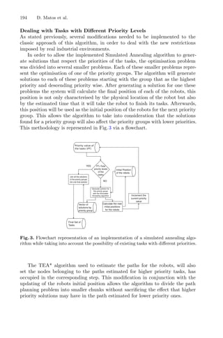

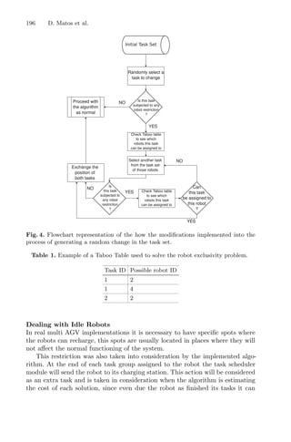
![Multiple Mobile Robots Scheduling Based on Simulated Annealing 197
still interfere with the normal functioning of the other robots and cause pathing
conflicts.
To prevent the robots from moving to their charging stations before finishing
all their tasks, this task will be permanently fixed as the last task to be executed
by each of the robots. It will also be outside the scope of the normal random
change process that occurs in the Simulated Annealing algorithm, therefore pre-
venting any change, induced by the algorithm into the task set, from altering its
position in the task set.
5 Tests and Results
In this section the test description and results obtained during this study will
be described and displayed. As stated before, the objective of this study is to
determine the efficiency and suitability of the Simulated Annealing algorithm
when it is used to optimise the task scheduling of a multi AGV system.
The Simulated Annealing algorithm will be analysed based on two key factors.
The overall cost of the final path generated by the algorithm and the time it took
the algorithm to reach said solution. The performance of this algorithm will be
compared to the case where the task are randomly distributed and to the case
where the tasks are optimised to reduce the distance travelled between each task
without taking into account possible path planning conflicts.
5.1 Test Parameters and Environment
In order to tests the efficiency of the different methodologies, the map used in
[19] was chosen has the test environment. This map defines a real life map of
an industrial implementation of a multi AGV system and has as its dimensions
110 × 80 m. This map is represented in Fig. 5.
Fig. 5. Map of the environment use for the tests [19]. The possible paths that the
robots can use are represented in the figure via the red coloured lines.](https://image.slidesharecdn.com/optimizationlearningalgorithmsandapplications-231204021346-9e8015c0/85/Optimization-Learning-Algorithms-and-Applications-pdf-209-320.jpg)

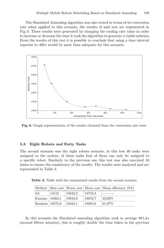
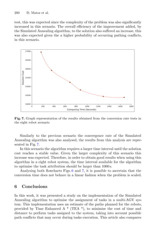
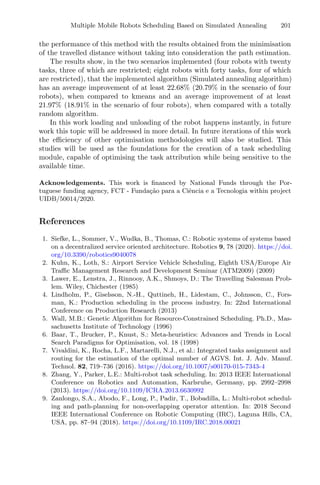

![Multi AGV Industrial Supervisory
System
Ana Cruz1(B)
, Diogo Matos2
, José Lima2,3
, Paulo Costa1,2
, and Pedro Costa1,2
1
Faculty of Engineering, University of Porto, Porto, Portugal
up201606324@edu.fe.up.pt, {paco,pedrogc}@fe.up.pt
2
INESC-TEC - INESC Technology and Science, Porto, Portugal
diogo.m.matos@inesctec.pt
3
Research Centre of Digitalization and Intelligent Robotics,
Instituto Politécnico de Bragança, Bragança, Portugal
jllima@ipb.pt
Abstract. Automated guided vehicles (AGV) represent a key element in
industries’ intralogistics and the use of AGV fleets bring multiple advan-
tages. Nevertheless, coordinating a fleet of AGV is already a complex
task but when exposed to delays in the trajectory and communication
faults it can represent a threat, compromising the safety, productivity
and efficiency of these systems. Concerning this matter, trajectory plan-
ning algorithms allied with supervisory systems have been studied and
developed. This article aims to, based on work developed previously,
implement and test a Multi AGV Supervisory System on real robots and
analyse how the system responds to the dynamic of a real environment,
analysing its intervention, what influences it and how the execution time
is affected.
Keywords: Multi AGV coordination · Time enhanced A* · Real
implementation
1 Introduction
Automated guided vehicle systems (AGVS), a flexible automatic mean of con-
veyance, have become a key element in industries’ intralogistics, with more indus-
tries making use of AGVS since the mid-1990s [13]. These systems can assist to
move and transport items in manufacturing facilities, warehouses, and distribu-
tion centres without any permanent conveying system or manual intervention. It
follows configurable guide paths for optimisation of storage, picking, and trans-
port in the environment of premium space [1].
The use of AGV represents a significant reduction of labour cost, an increase
in safety and the sought-after increase of efficiency. By replacing a human worker
with an AGV, a single expense for the equipment is paid- the initial investment-
avoiding the ongoing costs that would come with a new hire [2]. These sys-
tems are also programmed to take over repetitive and fatiguing tasks that could
c
Springer Nature Switzerland AG 2021
A. I. Pereira et al. (Eds.): OL2A 2021, CCIS 1488, pp. 203–218, 2021.
https://doi.org/10.1007/978-3-030-91885-9_15](https://image.slidesharecdn.com/optimizationlearningalgorithmsandapplications-231204021346-9e8015c0/85/Optimization-Learning-Algorithms-and-Applications-pdf-215-320.jpg)
![204 A. Cruz et al.
diminish the human worker attention and lead to possible accidents. Therefore,
industries that use AGV can significantly reduce these accidents and, with a
24 h per day and 7 days per week operability and high production output, AGV
ensure worker safety while maximizing production [3].
Multiple robot systems can accomplish tasks that no single robot can accom-
plish, since a single robot, no matter how capable it is, is spatially limited [5].
Nevertheless, a multi-AGV environment requires special attention. Coordinat-
ing a fleet of AGV is already a complex task and restrict environments with the
possibility of exposing the AGV to delays in the trajectory and even communi-
cation faults can represent a threat, compromising the safety, productivity and
efficiency of these systems. To solve this, trajectory planning algorithms allied
with supervisory systems have been studied and developed. Based on the work
developed by [8], it is intended to implement and test a Multi AGV Supervisory
System on real robots and analyse how the system responds to the dynamic of
a real environment.
This paper aims to analyse the intervention of the implemented Supervisory
Module, what influences it and how the execution time is affected considering
other variables such as the robots’ velocity.
2 Literature Review
The system performance is highly connected with path planning and trajectory
planning. Path planning describes geometrically and mathematically the way
from the starting point to the destination point, avoiding collisions with obsta-
cles. On the other hand, trajectory planning is that path as a function of time:
for each time instance, it defines where the robot must be positioned [7].
When choosing a path planning method, several aspects have to be consid-
ered such as the type of intended optimisation (path length, execution time),
computational complexity and even if it is complete (always finds a solution
when it exists), in full resolution (there is a solution to a particular discretisa-
tion of the environment) or probabilistically complete (the probability of finding
a solution converges to 1 as the time tends to infinity) [7].
When it comes to coordinating a multi-AGV environment, the Time
Enhanced A* (TEA*) Algorithm revealed to be very fitted as it is described
as a multi-mission algorithm that incrementally builds the path of each vehicle
considering the movements of the others [10].
2.1 TEA* Algorithm
The TEA* Algorithm is a graph search algorithm, based on the A* algorithm,
developed by [10]. This approach aims to fulfil industrial needs by creating routes
that minimise the time allocated for each task, avoid collisions between AGV
and prevent the occurrence of deadlocks.
Considering a graph G with a set of vertexes V and edges E (links between
the vertexes), with a representation of the time k = [0; TMax], each AGV can](https://image.slidesharecdn.com/optimizationlearningalgorithmsandapplications-231204021346-9e8015c0/85/Optimization-Learning-Algorithms-and-Applications-pdf-216-320.jpg)
![Multi AGV Industrial Supervisory System 205
Fig. 1. TEA* algorithm: input map and analysed neighbour cells focusing on the cell
with the AGV’s position [11]
only start and stop in vertexes and a vertex can only be occupied by one vehicle
at a temporal layer [11]. As it can be seen in Fig. 1, the analysed neighbour cells
belong to the next temporal layer and include the cell containing the AGV’s
current position.
To find the minimal path, the algorithm starts by calculating the position
of each robot in each temporal layer and the next analysed neighbour cell is
dependent on a cost function. In the TEA* approach, the heuristic function
used is the euclidean distance. Hence, in the future, possible collisions can be
identified and avoided in the beginning (k = 0) of the paths’ calculation [10].
Since the coordination between robots is essential to avoid collisions and to
guarantee the correct execution of the missions, this approach ensures it since
the previously calculated paths become moving obstacles [10].
Combining this approach with a supervisory system revealed to be a more
efficient approach to avoid collisions and deadlocks [8]. Instead of executing
the TEA* methodology as an online method (the paths are re-calculated every
execution cycle, a computationally heavy procedure), the supervisory system
would detect delays in the communication, deviations in the routes of the robots
and communication faults and trigger the re-calculation of the paths, if needed.
Therefore, [8] proposed a supervisory system consisting of two modules: Plan-
ning Supervision Sub-Module and Communication Supervision Sub-Module.
3 System Overall Structure
To implement and test the work developed by [8], and further modifications, it
was set a shop floor map and developed a fleet of three robots and their control
module, a localisation system based on the pose estimation of fiducial markers
and a central control module.
The architecture of the system developed is represented in Fig. 2.
The Central Control Module of the system is composed of three hierarchical
modules: the Path Planning Module (TEA* Algorithm) and the Supervisory
Module: the Planning Supervision and the Communication Supervision.](https://image.slidesharecdn.com/optimizationlearningalgorithmsandapplications-231204021346-9e8015c0/85/Optimization-Learning-Algorithms-and-Applications-pdf-217-320.jpg)
![206 A. Cruz et al.
Robot Localisation
Module
Robot Control Module
Path Planning (TEA* Algorithm)
Planning Supervision
Communication
Supervision
Central Control Module
Fig. 2. System architecture and relations between the different modules
The Robot Localisation Module locates and estimates the robot’s coordinates
and communicates simultaneously with the Central Control Module and the
Robot Control Module.
Lastly, the Robot Control Module is responsible for calculating and deliv-
ering through UDP packets the most suitable velocities for each robots’ wheel,
depending on the destination point/node indicated by the Central Control Mod-
ule.
The communication protocol used, UDP (User Datagram Protocol), is
responsible for establishing low-latency and loss-tolerating connections between
applications on the internet. Because it enables the transfer of data before an
agreement, provided by the receiving party, the transmissions are faster. As a
consequence, UDP is beneficial in time-sensitive communications [12].
3.1 Robot Localisation Module
To run the system, the current coordinates, X and Y, and orientation, Theta,
of the robots were crucial. Suitable approaches would be odometry or even an
Extended Kalman Filter localisation using beacons [4]. However, for pose esti-
mation, the Robot Localisation Module applies a computer vision algorithm. For
this purpose, a camera was set above the centre of the shop floor map and the
robots were identified with ArUco markers [6,9], as represented in Fig. 3.
The ArUco marker is a square marker characterised by a wide black border
and an inner binary matrix that determines its identifier. Using the ArUco library
developed by [9] and [6] and associating an ArUco tag id to each robot, it was
possible to obtain the coordinates of the robots’ positions with less than 2 cm
of error. However, the vision algorithm revealed to be very sensitive to poor](https://image.slidesharecdn.com/optimizationlearningalgorithmsandapplications-231204021346-9e8015c0/85/Optimization-Learning-Algorithms-and-Applications-pdf-218-320.jpg)
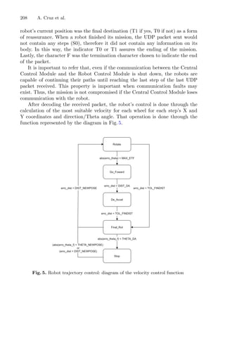
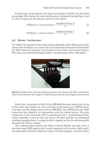
![210 A. Cruz et al.
ESP32
DRV8825
Stepper motor
NEMA
DRV8825
Stepper motor
NEMA
Vbat
Off
control
3 x
18650
R
Wheel
L
Wheel
Push-button Power Switch
Fig. 7. Robot architecture’s diagram: Black lines represent control signals and red lines
represent power supply. (Color figure online)
is placed on each wheel. Beyond the two wheels, a free contact support of Teflon
with low friction is used to support the robot.
3.4 Central Control Module
As explained previously, the Central Control Module is the main module and the
one responsible for running the TEA* algorithm with the help of its supervisory
system.
Supervisory System. The supervisory system proposed by [8] is responsible
for deciding when to re-plan the robots’ paths and for detecting and handling
communications faults through two sub-modules hierarchically related with each
other: these modules are referred to as the Planning Supervision Sub-Module and
the Communication Supervision Sub-Module.
In environments where no communication faults are present, the Planning
Supervision Sub-Module is responsible for determining when one of the robots is
delayed or ahead of time (according to the path planned by the TEA* algorithm)
and also detect when a robot has completed the current step of its path.
On the other hand, the Communication Supervision Sub-Module is only
responsible for detecting communication faults. When a communication fault
is detected, the Planning Supervision Sub-Module is overruled and the re-
calculation of the robots’ paths is controlled by the Communication Supervi-
sion Sub-Module. Once the communication is reestablished, the supervision is
returned to the Planning Supervision Sub-Module.](https://image.slidesharecdn.com/optimizationlearningalgorithmsandapplications-231204021346-9e8015c0/85/Optimization-Learning-Algorithms-and-Applications-pdf-222-320.jpg)
![Multi AGV Industrial Supervisory System 211
In the Central Control Module, after the initial calculation of the robot’s
paths, done by the Path Planning Module, the Planning Supervision Module
is responsible for checking three critical situations that can lead to collisions
and/or deadlocks:
– If a robot is too distant from its planned position;
– If the maximum difference between steps is 1;
– If there is a robot moving into a position currently occupied by other.
All these situations could be covered in only one: verifying when the robots
become unsynchronised. If the robots are not synchronised, it means that each
robot is at a different step of the planned path, which can lead to collisions and
deadlocks. However, triggering the supervisory system by this criterion may lead
to an ineffective system where the paths are constantly being recalculated.
In the next section are described the tests performed to study the impact of
the supervisor and, consequently, how the re-planning of the robot’s path affects
the execution’s time and the number of tasks completed and what influences the
supervisor.
4 Experiments and Results
The shop floor map designed is presented in Fig. 8. This map was turned into a
graph with links around the size of the robot plus a safety margin, in this case,
the links measure, approximately, 15 cm.
Fig. 8. Shop floor map designed to validate the work developed
The decomposition of the map was done using the Map Decomposition Mod-
ule, developed by [8], and incorporated in the Central Control Module through
an XML file.
To test the Planning Supervision Sub-Module and its intervention, it was
assigned a workstation to each robot as written in Table 1. After reaching the
workstation, each robot moves towards the nearest rest station, which is any
other station that is not chosen as a workstation. In Fig. 9, it is possible to
observe the chosen workstations in blue and the available rest stations in red.](https://image.slidesharecdn.com/optimizationlearningalgorithmsandapplications-231204021346-9e8015c0/85/Optimization-Learning-Algorithms-and-Applications-pdf-223-320.jpg)
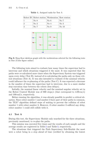

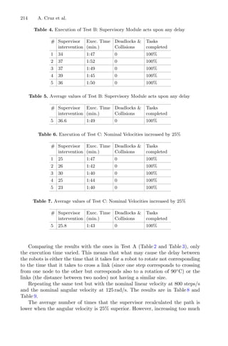
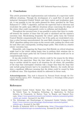

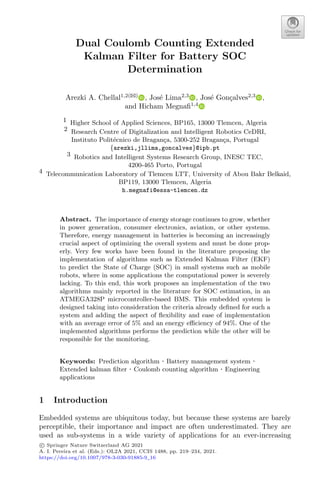
![220 A. A. Chellal et al.
diversity of functions [1]. Whether it is a hybrid vehicle, a solar power plant,
or any other everyday electrical device (PC, smartphone, drone...), the key ele-
ment remains the ability to monitor, control and optimise the performance of
one or more modules of these batteries, this type of device is often referred to
as a Battery Management System (BMS). A BMS is one of the basic units of
electrical energy storage systems, a variety of already developed algorithms can
be applied to define the main states of the battery, among others: SOC, state of
health (SOH) and state of functions (SOF) that allow real-time management of
the batteries.
For the BMS to provide optimal monitoring, it must operate in a noisy envi-
ronment, it must be able to electrically disconnect the battery at any time, it
must be cell-based and perform uniform charging and discharging across all cells
in the battery [2], and the components used must be able to withstand at least
the total current drawn by the load [3]. In addition, it must continuously monitor
various parameters that can greatly influence the battery, such as cell tempera-
ture, cell terminal voltage and cell current. This embedded system must be able
to notify the robot using the battery to either stop drawing energy from it, or
to go to the nearest charging station.
However, in the field of mobile robotics and small consumer devices, such as
Smarthpones or Laptops, as there are no requirements regarding the accuracy to
which a BMS must be held, the standard approach such as Open Circuit Volt-
age (OCV) and Coulomb Counting (CC) methods are generally applied, this is
mainly due to the fact that the use of more complicated estimation algorithms
such as EKF, Sliding Mode and Machine Learning [4,5] requires higher compu-
tational power, thus, the most advanced battery management system algorithms
reported in the literature are developed and verified by laboratory experiments
using PC-based software such as MATLAB and controllers such as dSPACE.
As an additional information, the most widely used battery systems in robotics
today are based on electrochemical batteries, particularly lithium-ion technolo-
gies with polymer as an Electrolyte [6].
This document is devided into 5 sections, the rest of the paper is structured as
follow. Section 2 promotes the work already done in this field and highlights the
objectives intended throught this work. Section 3 offer a brief algorithm descrip-
tion implemented on the prototype. Section 4, describes the proposed solution
for the system, where a block diagram and several other diagrams defining the
operating principle are offered. Section 5 provides the results and offer some dis-
cussion. Finally, Sect. 5 draws together the main ideas described in this article
and outlines future prospects for the development of this prototype.
2 State of the Art Review
Several research teams around the world have proposed different solutions to
design an efficient BMS system for lithium-ion batteries. Taborelli et al. have
proposed in [7], a design of an EKF and Ascending Extended Kalman Filter
(AEKF) algorithms specifically developed for light vehicle categories, such as](https://image.slidesharecdn.com/optimizationlearningalgorithmsandapplications-231204021346-9e8015c0/85/Optimization-Learning-Algorithms-and-Applications-pdf-232-320.jpg)
![DCC-EKF Battery SOC Determination 221
electric bicycles, in which a capacity prediction algorithm is also implemented
tackling SOH estimation. The design has been validated by using simulation
software and real data acquisition. In [8], Mouna et al. implemented two EKF
and sliding mode algorithms in an Arduino board for SOC estimation, using
an equivalent first-order battery as a model. Validation is performed by data
acquisition from Matlab/Simulink. Sanguino et al. proposed in [9] an alterna-
tive design for battery system, where two batteries works alternatively, one of
the batteries is charged through solar panels installed on the top of the VAN-
TER mobile robot, while the other one provides the energy to the device. The
battery SOC selection is performed following an OCV check only and the SOC
monitoring is done by a coulomb counting method.
In addition, several devices are massively marketed, these products are used
in different systems, from the smallest to the largest. The Battery Management
System 4–15S is a BMS marketed by REC, it has the usual battery protec-
tions (temperature, overcurrent, overvoltage) [10]. A cell internal DC resistance
measurement technique is applied, suggesting the application of a simple resis-
tor equivalent model and an open circuit voltage technique for SOC prediction,
and an Coulomb counting technique for SOC monitoring. The device can be
operated as a stand-alone unit and offers the possibility of being connected to
a computer with an RS-485 for data export. This device is intended for use in
solar system. Roboteq’s BMS10x0 is a BMS and protection system for robotic
devices developed by Roboteq, it uses a 32-bit ARM Cortex processor and offers
the typical features of a BMS, along with Bluetooth compatibility for wireless
states checking. It can monitor from 6 to 15 batteries at the same time. Voltage
and temperature thresholds are assigned based on the chemical composition of
the battery. The SOC is calculated based on an OCV and CC techniques [11].
To the best of the authors’ knowledge, all research in the field of EKF-
based BMS is based on bench-scale experiments using powerful softwares, such
as MATLAB, for data processing. So far, the constraint of computational power
limitation is not really addressed in the majority of scientific papers dealing with
this subject. This paper focus on the implementation of an Extended Kalman
Filter helped with a Coulomb Counting technique, called DCC-EKF, as a SOC
and SOH estimator in ATMEGA328P microcontrollers, the proposed system is
self powered, polyvalent to all types of Lithium cells, easy to plug with other
systems and take into consideration most of the BMS criteria reported in the
literature.
3 Algorithm Description
There are many methods reported in the literature that can give a represen-
tation of the actual battery charge [4,5,7,8]. However, these methods vary in
the complexity of the implementation and the accuracy of the predicted results
over long term use. There is a correlation between these two parameters, as the
complexity of an algorithm increases, so does the accuracy of the results.
Also, simulation is a very common technique for evaluating and validating
approaches and allows for rapid prototyping [1]; these simulations are based on](https://image.slidesharecdn.com/optimizationlearningalgorithmsandapplications-231204021346-9e8015c0/85/Optimization-Learning-Algorithms-and-Applications-pdf-233-320.jpg)
![222 A. A. Chellal et al.
models that are approximations of reality. MATLAB is a modeling and sim-
ulation tool based on mathematical models, provided with various tools and
libraries. In this section, the two algorithms applied in the development of this
prototype will be described and the results of the simulation performed for the
extended Kalman filter algorithm will be given.
3.1 Coulomb Counting Method
The Coulomb counting method consist of a current measurement and integration
in a specific period of time. The evolution of the state of charge for this method,
can be described by the following expression:
SOC(tn) = SOC(tn−1) +
nf
Cactual
tn−1
tn
I · dt (1)
where, I is the current flowing by the battery, Cactual is the actual total storable
energy in the battery and nf represents the faradic efficiency.
Although this method is one of the most widely used methods for monitor-
ing the condition of batteries and offers the most accurate results if properly
initialized, it has several drawbacks that lead to errors. The coulomb counting
method is an open-loop method and its accuracy is therefore strongly influenced
by accumulated errors, which are produced by the incorrect initial determina-
tion of the faradic efficiency, the battery capacity and the SOC estimation error
[12], making it very rarely applied on its own. In addition, the sampling time
is critical and should be kept as low as possible, making applications where the
current varies rapidly unadvisable with this method.
3.2 Extended Kalman Filter Method
Since 1960, Kalman Filter (KF) has been the subject of extensive research and
applications, the KF Algorithm estimates the states of the system from indirect
and uncertain measurements of the system’s input and output. The general
discrete time representation of it, is represented as follow:
xk = Ak−1 · xk−1 + Bk−1 · uk−1 + ωk
yk = Ck · xk + Dk · uk + υk
(2)
Where, xk ∈ Rn×1
is the state vector, Ak ∈ Rnxn
is the system matrix in
discrete time, yk ∈ Rm × 1 is the output, uk ∈ Rm×1
is the input, Bk ∈ Rnxm
is the input matrix in discrete time, and Ck ∈ Rm×n
is the output matrix in
discrete time. ω and υ represents the Gaussian distributed noise of the process
and measurement.
However, Eq. 2 is only valid for linear systems, in the case of nonlinear systems
such as batteries, the EKF is applied to include the non-linear behaviour and
to determine the states of the system [14]. The EKF equation has the following
form:
xk+1 = f(xk, uk) + ωk
yk = h(xk, uk) + υk
(3)](https://image.slidesharecdn.com/optimizationlearningalgorithmsandapplications-231204021346-9e8015c0/85/Optimization-Learning-Algorithms-and-Applications-pdf-234-320.jpg)
![DCC-EKF Battery SOC Determination 223
Where,
Ak =
∂f(xk, uk)
∂xk
, Ck =
∂h(xk, uk)
∂xk
(4)
After initialization, the EKF Algorithm always goes through two steps, predic-
tion and correction. The KF is extensively detailed in many references [13–15], we
will therefore not focus on its detailed description. The Algorithm 1 summarize
the EKF function implemented in each Slave ATMEGA328P microcontroller,
the matrices Ak, Bk, Ck, Dk, xk are discussed in Sect. 3.3.
Algorithm 1: Extended Kalman Filter Function
initialise A0, B0, C0, D0, P0, I0, x0, Q and R ;
while EKF Called do
Ik measurements; Vtk measurements;
ˆ
xk = Ak−1 . xk−1 + Bk−1 . Ik−1 ;
ˆ
Pk = Ak−1 . Pk−1 . At
k−1 + Q ;
ˆ
Pk not diagonal = 0;
if ˆ
SOCk ∈[SOC interval] then
Rt, Rp and Cp updated;
end
Ck = V oc( ˆ
SOCk) + V̂Pk ;
Dk = Rt;
V̂tk = Ck + Dk · Ik;
L = (Ck · ˆ
Pk · Ct
k + R);
if L = 0 then
Kk = ˆ
Pk · Ct
k / L;
end
xk = ˆ
xk + Kk · (Vtk − V̂tk );
Pk = (I − Kk · Ck) · ˆ
Pk;
Pk not diagonal = 0;
k = k + 1;
Result: Send xk
end
The overall performance of the filters is set by the covariance matrix P,
the process noise matrix Q and the measurement noise R. The choice of these
parameters were defined throught experience and empirical experiment and are
given by:
Q =
0.25 0
0 0
, P =
1 0
0 1
and R = 0.00001
Data obtained from discharge tests of different cells simulations were applied to
verify the accuracy of this estimator with known parameters and are reported
in Sect. 3.4. The EKF Algorithm implemented in the ATMEGA328P microcon-
trollers has a sampling time of 0.04 s.](https://image.slidesharecdn.com/optimizationlearningalgorithmsandapplications-231204021346-9e8015c0/85/Optimization-Learning-Algorithms-and-Applications-pdf-235-320.jpg)

![DCC-EKF Battery SOC Determination 225
From the Eqs. 5, 7 and 8, it is possible to deduce the equation characterising
the behaviour of the battery, which is expressed as the following system:
⎧
⎪
⎪
⎪
⎨
⎪
⎪
⎪
⎩
.
SOC
.
Vp
=
0 0
0 −1
RpCp
·
SOC
Vp
+
1
Cactual
1
Cp
· I
Vt = poly 1 ·
SOC
Vp
+ Rt · I
(9)
Where, poly is the polynomial formula described in Eq. 6. Since the microcon-
troller processes actions in discrete events, the previous system must be tran-
scribed into its discrete form, which is written as follows,
⎧
⎪
⎪
⎪
⎨
⎪
⎪
⎪
⎩
.
SOC
.
Vp
=
1 0
0 exp −Δt
RpCp
·
SOC
Vp
k−1
+
1
Cactual
1
Cp
· Ik−1
Vt = poly 1 ·
SOC
Vp
k
+ Rt · Ik
(10)
From both Eqs. 2 and 10, it is deduced that the current I is the input of the
system, the voltage Vt is the output and the matrices Ak, Bk, Ck and Dk
matrices are given by:
Ak =
1 0
0 exp −Δt
RpCp
, Bk =
1
Cactual
1
Cp
, xk =
SOCk
VPk
, Ct
k =
poly
1
, Dk = Rt
3.4 Simulation Results
Given the large number of articles dealing with the validation of these algorithms
[13,16,17], it is however not necessary to dwell on this subject. Nevertheless, a
simulation of the algorithm is proposed in this section, in order to confirm the
good follow-up of the algorithm according to the chosen parameters.
Fig. 2. (a) overall Simulink model highlighting the Input/Output of the simulation (b)
Battery sub-system model](https://image.slidesharecdn.com/optimizationlearningalgorithmsandapplications-231204021346-9e8015c0/85/Optimization-Learning-Algorithms-and-Applications-pdf-237-320.jpg)
![226 A. A. Chellal et al.
The graphical representation of MATLAB/Simulink using graphical blocks
to represent mathematical and logical constructs and process flow is intuitive and
provides a clear focus on control and observation functions. Although Simulink
has been the tool of choice for much of the control industry for many years [18],
it is best to use Simulink only for modelling battery behaviour and not for the
prediction algorithm. The battery model presented before is applied as a base
model, the more complex model will not be able to simulate all possible cases
and will therefore increase the time needed for development. Figure 2 represents
the battery simulation used in MATLAB/Simulink.
Figure 3 shows a comparison of the state of charge of the battery with simu-
lation for the Extended Kalman filter, and a plot of the error with the real and
the predicted one. The test consists of a 180 s discharge period followed by a
one hour rest period, the cell starts fully charged and the EKF state of charge
indicator is set at 50% SOC.
Fig. 3. Estimated and reference SOC comparison with the absolute error of the SOC
for Extended Kalman Filter with a constant discharge test and a rest period.
The continuous updating of the correction gain (K), which is due to the
continuous re-transcription of the error covariance matrices, limits the divergence
as long as the SOC remains within the predefined operating range (80%-40%).
The response of the observer to the determination of the SOC can be very fast,
on the order of a few seconds. Also, from the previous figure it is clear that,
for known parameters, the SOC can be tracked accurately with less than 5% of
error, and record a perfect prediction for when the battery is at rest. Figure 4
shows the simulation results of a constant current discharge test.
Although a good SOC monitoring by the EKF, it still requires a good deter-
mination of the battery parameter. Some reported works [19,20], have proposed
the use simple algebraic method or a Dual Extended Kalman Filter (DEKF) as
an online parameter estimator, to estimate them on the fly. Unfortunately, these
methods require a lot of computational power, to achieve a low sampling time](https://image.slidesharecdn.com/optimizationlearningalgorithmsandapplications-231204021346-9e8015c0/85/Optimization-Learning-Algorithms-and-Applications-pdf-238-320.jpg)
![DCC-EKF Battery SOC Determination 227
Fig. 4. Estimated and reference SOC comparison with the absolute error of the SOC
for Extended Kalman Filter with a constant discharge test.
and reach convergence, which is difficult to achieve with a simple ATMEGA328P.
For this reason, and given the speed at which the EKF is able to determine the
battery SOC at rest, the EKF algorithm is applied to determine the battery SOC
at start-up and then the CC algorithm is applied to carry on the estimation.
4 Proposed Solution
The system is designed to be “Plug and Play”, with two energy input and output
located on one side only, future users of the product can quickly install and ini-
tialize the BMS, which works for all types of Lithium Model 18650 batteries, the
initialization part is described in more depth in the next section. The connecting
principle of the electronic components is illustrated in Fig. 5.
4.1 Module Connection
The Master microcontroller is the central element of the system, the ATMEL’s
ATMEGA328P was chosen for its operational character and low purchase cost,
it collect the State of Charge predicted by each ATMEGA328P slave micro-
controller and control the energy flow according to the data collected. This
microcontroller is connected to push buttons and an OLED screen to facili-
tate communication with the user. Power is supplied directly from the batteries,
the voltage is stabilised and regulated for the BMS electronics by an step down
voltage regulator.
The Inter-Integrated Circuit (I2C) is a bus interface connection using only
2 pins for data transfer, it is incorporated into many devices and is ideal for
attaching low-speed peripherals to a motherboard or embedded system over a
short distance, it provides a connection-oriented communication with acknowl-
edge [21]. Figure 6 represent the electronic circuit schematic diagram.](https://image.slidesharecdn.com/optimizationlearningalgorithmsandapplications-231204021346-9e8015c0/85/Optimization-Learning-Algorithms-and-Applications-pdf-239-320.jpg)
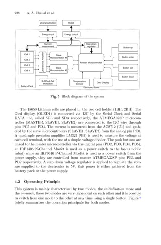
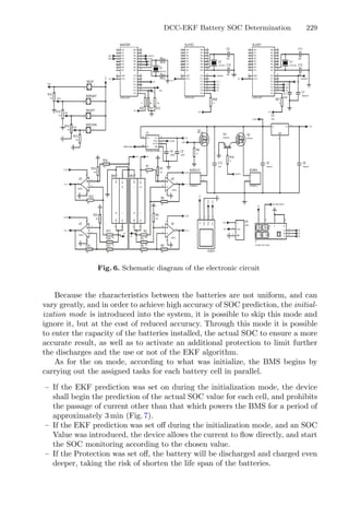
![230 A. A. Chellal et al.
Begin of
Initialisation mode
Display menu
Arrow Navigation
(UP DOWN)
buttons
1- Initialisation of cell
capacity
2- (Des)activate the
EKF
4- (Des)activate the
cell protection
3- Enter Manualy the
SOC
Selected ?
5- Finish Initialisation
1
Selected ? Selected ? Selected ? Selected ?
Selection of the value
Value
selected ?
Yes/No Selection of the value Yes/No
2
Choice
selected ?
Value
selected ?
Choice
selected ?
Yes Yes Yes Yes Yes
Yes
Yes Yes Yes
2
EKF function,
Does not allow (dis)charge
3 minutes
Allow (dis)charge,
Coulomb Counting
function
SOCmin SOC SOCmax
Calculate R0
Yes
SOC SOCmin
No
No
Does not allow
discharge
Does not allow
charge
T passed
Send data to the
slave µ-controller
Yes
Yes
(b)
(a)
Fig. 7. Flow chart of the system algorithm. (a) Initialisation mode flow chart. (b)
On-mode flow chart with EKF algorithm activated.
The battery states are determined for each cell independently of the others
by a specific microcontroller assigned to it, and works with the principle of
Master/Slave communication. In order to keep a low sampling time, one slave
microcontroller is assigned to two batteries, reaching a sampling time of 0.085 s.
5 Results and Discussions
The result is the design of a BMS that takes into account the already established
requirements for this type of system and defines new ones, such as flexibility
and size, that must be met for mobile robots. A breadboard conception was first
carried out to perform the first tests. After power up, the initialisation mode is
first started as expected. After that, while the on-mode is running, the voltage,
current and SOC data are displayed on the screen, an accuracy of 100 mV and
40 mA is achieved. When the cell is at rest and for a SOC ∈ [80% − −40%], the
EKF prediction reaches an error of 5% in the worst case, for SOC cells above
80% the accuracy drops to 8%, while for SOC below 30% the algorithm diverges
completely (Fig. 10). These results are quite understandable, as the linearization
of these curves is done in only 10 points. A cell protection is performed by an
external circuit based on a S-8254A, it includes a high accuracy voltage detection
for lithium battery, avoiding over voltage while charging the batteries, they are
widely applied in rechargeable battery pack, due to their low costs and good
caracteristics [22].](https://image.slidesharecdn.com/optimizationlearningalgorithmsandapplications-231204021346-9e8015c0/85/Optimization-Learning-Algorithms-and-Applications-pdf-242-320.jpg)
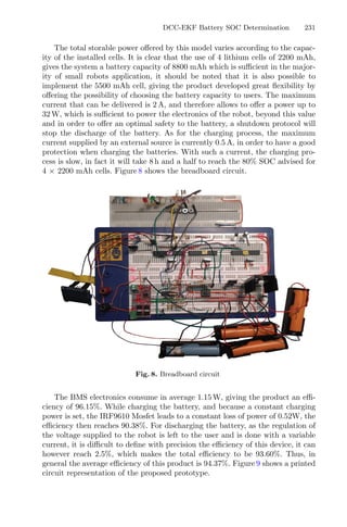
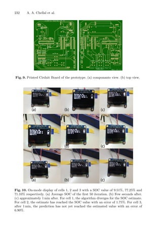


![Sensor Fusion for Mobile Robot
Localization Using Extended Kalman
Filter, UWB ToF and ArUco Markers
Sı́lvia Faria1(B)
, José Lima2,3
, and Paulo Costa1,3
1
Faculty of Engineering, University of Porto, Porto, Portugal
{up201603368,paco}@fe.up.pt
2
Research Centre of Digitalization and Intelligent Robotics,
Instituto Politécnico de Bragança, Bragança, Portugal
jllima@ipb.pt
3
INESC-TEC - INESC Technology and Science, Porto, Portugal
Abstract. The ability to locate a robot is one of the main features to
be truly autonomous. Different methodologies can be used to determine
robots location as accurately as possible, however these methodologies
present several problems in some circumstances. One of these problems
is the existence of uncertainty in the sensing of the robot. To solve this
problem, it is necessary to combine the uncertain information correctly.
In this way, it is possible to have a system that allows a more robust
localization of the robot, more tolerant to failures and disturbances. This
paper evaluates an Extended Kalman Filter (EKF) that fuses odometry
information with Ultra-WideBand Time-of-Flight (UWB ToF) measure-
ments and camera measurements from the detection of ArUco markers
in the environment. The proposed system is validated in a real envi-
ronment with a differential robot developed for this purpose, and the
achieved results are promising.
Keywords: ArUco markers · Autonomous mobile robot · Extended
kalman filter · Localization · Ultra-WideBand · Vision based system
1 Introduction
In a semi-structured environment a mobile robot needs to be able to locate itself
without human intervention, i.e. autonomously. It can be assumed that if the
robot knows its own pose (position and orientation), it can be truly autonomous
to execute given tasks. Since the first mobile robot was invented, the problem
of pose determination has been addressed by many researches and developers
around the world due to its complexity and the multitude of possible approaches.
The localization methods can be classified in two great categories: rela-
tive methods and absolute methods [1]. Relative localization methods gives the
robot’s pose relative to the initial one and for this purpose dead reckoning meth-
ods such as odometry and inertial navigation are used. Odometry is a technique
c
Springer Nature Switzerland AG 2021
A. I. Pereira et al. (Eds.): OL2A 2021, CCIS 1488, pp. 235–250, 2021.
https://doi.org/10.1007/978-3-030-91885-9_17](https://image.slidesharecdn.com/optimizationlearningalgorithmsandapplications-231204021346-9e8015c0/85/Optimization-Learning-Algorithms-and-Applications-pdf-247-320.jpg)
![Sensor Fusion for Mobile Robot Localization 237
– Dead Reckoning (DR): DR can approximately determine robot’s pose
using Odometry or Inertial Measurement Unit (IMU) by integration of the
pose from encoders and inertial sensors. This is one of the first methodology
used to calculate the robot position. Dead reckoning can give accurate infor-
mation on position, but is subject to cumulative errors over a long distances,
in that it needs to utilize the previous position to estimate the next relative
one and during which, the drift, the wheel slippage, the uneven floor and the
uncertainty about the structure of the robot will together cause errors. In
order to improve accuracy and reduce error, DR need to use other methods
to adjusts the position after each interval [2].
– Range-Based: Range-Based localization measures the distance and/or angle
to a natural or artificial landmarks. High accuracy measurements are critical
for in-building applications such as autonomous robotic navigation. Typically,
reference points, i.e. anchors, and their distance and/or angle to one or more
nodes of interest are used with in order to estimate a given pose. These
reference points are normally static or with an a priori map. There are several
methods that are used to perform the distances and angles calculations: Angle
of Arrival (AoA), Time of Flight (ToF), Time Difference of Arrival (TDoA)
and Received Signal Strength Indication (RSSI) [4]. The robot’s position can
be calculated with various technologies such as Ultra-WideBand (UWB) tags,
Radio Frequency Identification (RFID) tags, Laser Range Finders. This type
of localization is widely used in Wireless Sensors Network Localization. It
is important to mention that UWB is a wireless radio technology primarily
used in communications that has lately received more attention in localization
applications and that promises to outperform many of the indoor localization
methods currently available [2]. In [5], the authors proposed a method that
uses Particle Filter to fuse odometry with UWB range measurements, which
lacks the orientation, to obtain an estimate of the real-time posture of a robot
with wheels in an indoor environment.
– Visual-Based Systems: These systems can locate a robot by extracting
images of its environment using a camera. These systems can be Fiducial
marker systems that detect some markers in the environment by using com-
puter vision tools. These systems are useful for Augmented Reality (AR),
robot navigation and applications where the relative pose between camera
and object is required, due to their high accuracy, robustness and speed [7].
Several fiducial marker systems have been proposed in the literature such
as ARSTudio, ARToolkit and ARTag. However, currently the most popular
marker system in academic literature is probably the ArUco which is based
on ARTag and comes with an OpenSource library OpenCV of functions for
detecting and locating markers developed by Rafael Muñoz and Sergio Gar-
rido [6]. In addition, several types of research have been successfully conducted
based on this type of system, such as [6,8,9].
All of the aforementioned technologies can be used independently. However
they can also be used at the same time in order to combine the advantages
of each of them. By the proper fusion of these technologies in a multi-sensor](https://image.slidesharecdn.com/optimizationlearningalgorithmsandapplications-231204021346-9e8015c0/85/Optimization-Learning-Algorithms-and-Applications-pdf-249-320.jpg)
![238 S. Faria et al.
environment a more accurate and robust system can be achieved. For nonlinear
systems this fusion can be achieved through developed algorithms such as the
Extend Kalman Filter (EKF), the Unscented Kalman Filter (UKF) and the
Particle Filter, which are among the most widely used [3].
The presented work uses a combination of odometry, UWB ToF measured
distance and ArUco measured angle to compute an accurate pose of a robot, i.e.
position and orientation. The combination of the measures mentioned above is
achieved by an EKF, since it is the least complex and computationally efficient
algorithm.
3 System Architecture
The system architecture proposed for this work, and its data flow is represented
in Fig. 1. The system consists of two main blocks: Remote Computer and Real
Robot. For all tests performed, a real robot was used and adapted, which was
previously developed for other projects.
Fig. 1. System architecture proposed
The robot has a differential wheel drive system and therefore has two drive
wheels, which are coupled to independent stepper motors powered by Allegro
MicroSystems drivers - A4988, and a castor wheel, which has a support function.
The robot sizes 0.31 m × 0.22 m and is powered by an on-board 12 V battery and
a DC/DC step-down converter to supply the electronic modules, i.e. a Raspberry
Pi 3 Model B and Arduino microcontroller boards. The top level consists of a
Raspberry Pi that runs the raspbian operative system and is responsible for
receiving data from Pozyx system obtained through the Arduino 2 and receiving
data from Arduino 1 that corresponds to the speed and voltage of the motors and
battery current. All the data is then send over Wi-Fi to the Remote Computer,
where it is performed the Kalman Filter and the appropriate speeds for each
wheel are calculated. A Raspberry Pi Camera Module is also connected to the
Raspberry that is tasked with acquiring positioning information from the ArUco
markers placed in the environment. This information is acquired by a script that
runs on the Raspberry Pi and is sent to the Remote Computer via Wi-Fi. A block
diagram of the robot architecture is presented in Fig. 2.](https://image.slidesharecdn.com/optimizationlearningalgorithmsandapplications-231204021346-9e8015c0/85/Optimization-Learning-Algorithms-and-Applications-pdf-250-320.jpg)
![240 S. Faria et al.
For the specific problem, the following assumptions were made:
– Since the robot only navigates on the ground, without any inclinations, it is
assumed that the robot navigates on a two-dimensional plane.
– The beacons positions, MB,i, are stationary and previously known.
– Every 40 ms the odometry values are available. This values will be used to
provide the system input uk =
vk ωk
T
and refers to the odometry variation
between k and k − 1 instants.
– ZB,i(k) = [rB,i] and ZB,i(k) = [φB,i], identifies the distance measurement
between the Pozyx tag and the Pozyx anchor i, and the angle measure-
ment between the Robot camera and the ArUco marker i, respectively, at
the instant k.
Fig. 4. 2D localization given measurements to beacons with a known position
4.1 ArUco Markers
As already mentioned, the system is capable of extracting angle measurements
from ArUco markers, arranged in the environment, relative to the referential
frame of the robot. Each of the markers has an associated identification number
that can be extracted when the marker is detected in an image, which distin-
guishes each reference point. Using the ArUco library provided, it is possible
to obtain the rotation and translation (x, y, z) of the ArUco reference frame to
the Camera reference frame (embedded in the robot). This allows to obtain the
angle φ from the marker to the robot, to be extracted by the Eq. 1.
φ = atan2(
x
z
) (1)
Since the movement of the robot is only in 2D, the height (y) of the marker
is ignored when making the calculations, thus having the angle exclusively as a
horizontal difference. Note that the camera has been calibrated with a chessboard
so that the measurements taken are reliable [12].](https://image.slidesharecdn.com/optimizationlearningalgorithmsandapplications-231204021346-9e8015c0/85/Optimization-Learning-Algorithms-and-Applications-pdf-252-320.jpg)
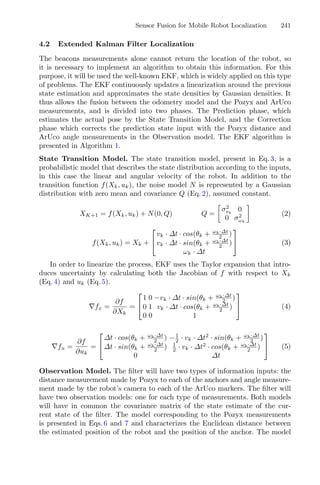
![242 S. Faria et al.
corresponding to the camera measurements, on the other hand, is presented in
Eqs. 9 and 10 and characterizes the angle between the robot’s referential and
the ArUco marker. Both measurements are affected by an additive Gaussian
noise with zero mean and covariance constant (R), a parameter related to the
characterization of the Pozyx error and the robot camera, respectively.
It should also be noted that, as for the state transition model, the EKF
algorithm also needs the Jacobian of h with respect to Xk (Eq. 8 and Eq. 11).
ZB,i = rB,i = h(MB,i, Xk) + N(0, R) R = [σ2
r ] (6)
ẐB,i = h(MB,i, X̂k) = (xB,i − x̂r,k)2 + (yB,i − ŷr,k)2 (7)
∇hx =
∂h
∂Xk
= −
xB,i−x̂r,k
√
(xB,i−x̂r,k)2+(yB,i−ŷr,k)2
−
yB,i−ŷr,k
√
(xB,i−x̂r,k)2+(yB,i−ŷr,k)2
0 (8)
ZB,i = φB,i = h(MB,i, Xk) + N(0, R) R = [σ2
φ] (9)
ẐB,i = h(MB,i, X̂k) = atan2(yB,i − ŷr,k, xB,i − x̂r,k) − θ̂r,k (10)
∇hx =
∂h
∂Xk
=
yB,i−ŷr,k
(xB,i−x̂r,k)2+(yB,i−ŷr,k)2 −
xB,i−x̂r,k
(xB,i−x̂r,k)2+(yB,i−ŷr,k)2 −1 (11)
Outlier Detection. Normally, when taking measurements with sensors, they
are prone to errors that can be generated due to hardware failures or unexpected
changes in the environment. For proper use of the measurements obtained, the
systems must be able to detect and deal with the less reliable measurements, i.e.,
those that deviate from the normal pattern and called outlier. Although there
are several approaches to solving this problem, but in the presence of multivari-
ate data, one of the common methods is to use the Mahalanobis Distance (MD)
(Eq. 12) as a statistical measure of the probability of some observation belonging
to a given data set. In this approach, outliers are removed as long as they are
outside a specific ellipse that symbolizes a specific probability in the distribu-
tion (Algorithm 2). In [10,11], it can be seen that this approach has been used
successfully in different applications, consisting of calculating the normalized
distance between a point and the entire population.
MD(x) = (x − μ)T · S−1 · (x − μ) (12)
In this case ẐB,i will be the population mean μ and S will be a factor rep-
resenting a combination of the state uncertainty and the actual sensor measure-
ment, present in line 8 of Algorithm 1. The choice of the threshold value can
be made by a simple analysis of the data or by determining some probabilistic
statistical parameter. In this case the threshold was established according to the](https://image.slidesharecdn.com/optimizationlearningalgorithmsandapplications-231204021346-9e8015c0/85/Optimization-Learning-Algorithms-and-Applications-pdf-254-320.jpg)
![Sensor Fusion for Mobile Robot Localization 243
Algorithm 1: EKF Localization Algorithm with known measurements
Input : X̂k, ZB,i, uk, Pk, R, Q
Output : X̂k+1, Pk+1
PREDICTION
1 X̂k+1 = f(X̂k, uk)
2 ∇fx = ∂f
∂Xk
3 ∇fu = ∂f
∂uk
4 Pk+1 = ∇fx · Pk · ∇fT
x + ∇fu · Q · ∇fT
u
CORRECTION
5 for i = 1 to NB do
6 ẐB,i = h(MB,i, X̂k)
7 ∇hx = ∂h
∂Xk
8 Sk,i = ∇hx · Pk · ∇hT
x + R
9 OutlierDetected = OutlierDetection(Sk,i, ẐB,i, ZB,i)
10 if not OutlierDetected then
11 Kk,i = Pk+1 · ∇hT
x · S−1
k,i
12 X̂k+1 = X̂k + Kk,i · [ZB,i − ẐB,i]
13 Pk+1 = [I − Kk,i · ∇hx] · Pk+1
14 end
15 end
χ2
probability table, so that observations with less than 5 % probability were
cut off in the case of the Pozyx system. For the ArUco system a threshold was
chosen so that observations with less than 2.5 % probability were cut off. These
values were chosen through several iterations of the algorithm, and the values,
which the algorithm behaved best for, were chosen.
Algorithm 2: Outliers Detection Algorithm
Input : Sk,i, ẐB,i, ZB,i
Output: OutlierDetected
1 MD(ZB,i) = (ZB,i − ẐB,i)T · S−1
k,i · (ZB,i − ẐB,i)
2 if MD(ZB,i) Threshold then
3 OutlierDetected = True
4 else
5 OutlierDetected = False
6 end
Pozyx Offset Correction. The Pozyx system distance measurements suffer
from different offsets, i.e. difference between the actual value and the measured
value, depending on how far the Pozyx tag is from a given anchor. These off-
sets also vary depending on the anchor at which the distance is measured, as](https://image.slidesharecdn.com/optimizationlearningalgorithmsandapplications-231204021346-9e8015c0/85/Optimization-Learning-Algorithms-and-Applications-pdf-255-320.jpg)
![244 S. Faria et al.
verified in Sect. 5.1. In order to correct this offset, the Algorithm 3 was imple-
mented. After calculating the estimated distance from the anchor to the robot
tag, it is verified between which predefined values this distance is, and then the
correction is made through a linear interpolation. The variable RealDist is an
array with a set of predefined distances for which the offsets have been deter-
mined. The variable Offset is a 4 × length(RealDist) matrix containing the
offsets corresponding to each distance for each of the four anchors placed in the
environment.
Algorithm 3: Offset Correction Algorithm
Input : ẐB,i
Output : ẐB,i
1 if ẐB,i = RealDist[0] then
2 ẐB,i = ẐB,i + Offset[i, 0]
3 else if ẐB,i = RealDist[7] then
4 ẐB,i = ẐB,i + Offset[i, 7]
5 else
6 for j = 0 to length(RealDist) − 1 do
7 if ẐB,i = RealDist[j] and ẐB,i = RealDist[j + 1] then
8 OffsetLin =
Offset[i, j] + Offset[i,j+1]−Offset[i,j]
RealDist[j+1]−RealDist[j]
· (ẐB,i − RealDist[j])
9 ẐB,i = ẐB,i + OffsetLin
10 end
11 end
12 end
5 Results and Discussion
The developed localization system was tested on the robot in a 2 m × 2 m
square area (Fig. 5). The output state X̂k+1 of the Kalman Filter allows con-
trolling the robot to follow the desired path. Pozyx anchors were placed at the
corners of the square and ArUco markers at the following (x, y) m positions:
(0, 0.5), (0, 1.5), (0.5, 2), (1.5, 2), (2, 1.5), (2, 0.5), (1.5, 0) and (0.5, 0). The initial
(x, y, θ) pose of the robot is (0.4, 0.5, 90◦
) and the robot moves in a clockwise
direction.
Before proceeding to the localization tests it was necessary to characterize
the error of both the Pozyx system and the ArUco system in order to be able to
correctly implement the algorithms discussed. When characterizing the perfor-
mance of systems it is important to realize that an error can have different sources
and can be of different types. The experiments performed in the characteriza-
tion of the systems will focus mainly on the analysis of accuracy and precision,](https://image.slidesharecdn.com/optimizationlearningalgorithmsandapplications-231204021346-9e8015c0/85/Optimization-Learning-Algorithms-and-Applications-pdf-256-320.jpg)
![Sensor Fusion for Mobile Robot Localization 245
Fig. 5. Robot map
which are typically associated with systematic and random errors respectively.
In the case of this particular work the characterization of sensor accuracy is
particularly important, since it will be used in the EKF to characterize the noise
measurement. Furthermore, accuracy measures how close the observations are
to real values, thus characterizing the existing offset.
5.1 Pozyx Characterization
In order to obtain a complete characterization of the Pozyx system and its
error, several experiments were performed in which distance measurements were
taken between the static anchors and the Pozyx tag. These experiments were
performed for different distances: [0.6, 0.8, 1, 1.2, 1.4, 1.6, 1.8, 2] m. It should also
be noted that both the anchors and the tag were at the same height from the
ground and that the real distance was measured with an appropriate laser. Thus
it was possible to conclude on the error/offset and standard deviation of the
measurements and verify their evolution depending on the distance between
anchor and tag.
Figure 6 shows the range of measurements for a distance between an anchor
and tag of 1.6 m. It can be concluded that the error of the Pozyx system follows
a Gaussian distribution.
Fig. 6. Distribution of Pozyx measurements for a distance of 1.6 m](https://image.slidesharecdn.com/optimizationlearningalgorithmsandapplications-231204021346-9e8015c0/85/Optimization-Learning-Algorithms-and-Applications-pdf-257-320.jpg)
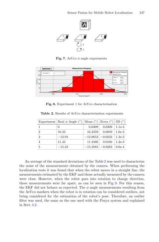
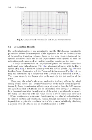
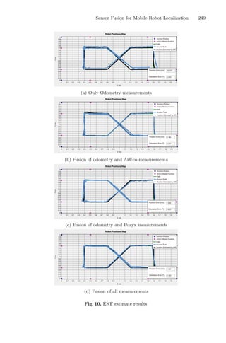
![Deep Reinforcement Learning Applied
to a Robotic Pick-and-Place Application
Natanael Magno Gomes1(B)
, Felipe N. Martins1
, José Lima2,3
,
and Heinrich Wörtche1,4
1
Sensors and Smart Systems Group, Institute of Engineering,
Hanze University of Applied Sciences, Groningen, The Netherlands
natanael gomes@msn.com
2
The Research Centre in Digitalization and Intelligent Robotics (CeDRI),
Polytechnic Institute of Bragança, Bragança, Portugal
3
Centre for Robotics in Industry and Intelligent Systems — INESC TEC,
Porto, Portugal
4
Department of Electrical Engineering, Eindhoven University of Technology,
Eindhoven, The Netherlands
Abstract. Industrial robot manipulators are widely used for repetitive
applications that require high precision, like pick-and-place. In many
cases, the movements of industrial robot manipulators are hard-coded or
manually defined, and need to be adjusted if the objects being manipu-
lated change position. To increase flexibility, an industrial robot should
be able to adjust its configuration in order to grasp objects in vari-
able/unknown positions. This can be achieved by off-the-shelf vision-
based solutions, but most require prior knowledge about each object to
be manipulated. To address this issue, this work presents a ROS-based
deep reinforcement learning solution to robotic grasping for a Collab-
orative Robot (Cobot) using a depth camera. The solution uses deep
Q-learning to process the color and depth images and generate a -
greedy policy used to define the robot action. The Q-values are esti-
mated using Convolutional Neural Network (CNN) based on pre-trained
models for feature extraction. Experiments were carried out in a sim-
ulated environment to compare the performance of four different pre-
trained CNN models (RexNext, MobileNet, MNASNet and DenseNet).
Results show that the best performance in our application was reached by
MobileNet, with an average of 84 % accuracy after training in simulated
environment.
Keywords: Cobots · Reinforcement learning · Computer vision ·
Pick-and-place · Grasping
1 Introduction
The usage of robots has been increasing in the industry for the past 50 years
[1], specially in repetitive tasks. Recently, industrial robots are being deployed
c
Springer Nature Switzerland AG 2021
A. I. Pereira et al. (Eds.): OL2A 2021, CCIS 1488, pp. 251–265, 2021.
https://doi.org/10.1007/978-3-030-91885-9_18](https://image.slidesharecdn.com/optimizationlearningalgorithmsandapplications-231204021346-9e8015c0/85/Optimization-Learning-Algorithms-and-Applications-pdf-263-320.jpg)
![252 N. M. Gomes et al.
in applications in which they share (part of) their working environment with
people. Those type of robots are often referred to as Cobots, and are equipped
with safety systems according to ISO/TS 15066:2016 [2]. Although Cobots are
easy to setup and program, their programs are usually written manually. If
there is a change in the position of objects in their workspace, which is common
when humans also interact with the scene, their program needs to be adjusted.
Therefore, to increase flexibility and to facilitate the implementation of robotic
automation, the robot should be able to adjust its configuration in order to
interact with objects in variable positions.
A Robot manipulator consists of a series of joints and links forming the arm,
at the far end are placed the end-effectors. The purpose of an end-effector is to
act on the environment, for example by manipulating objects in the scene. The
most common end-effector for grasping is the simple parallel gripper, consisting
of two-jaw design.
Grasping is a difficult task when different objects are not always in the same
position. To obtain a grasping position of the object, several techniques have
been applied. In [3] a vision technique is used to define candidate points in the
object and then triangulate one point where the object can be grasped.
With the evolution of the processing power, Computer Vision (CV) has also
played an important role in industrial automation for the last 30 years, including
depth images processing [4]. CV has been applied from food inspection [5,6] to
smartphone parts inspection [7]. Red Green Blue Depth (RGBD) cameras are
composed of a sensor capable of acquiring color and depth information and have
been used in robotics to increase the flexibility and bring new possibilities. There
are several models available e.g. Asus Xtion, Stereolabs ZED, Intel RealSense
and the well-known Microsoft Kinect. One approach to grasping different types
of objects using RBGD cameras is to create 3D templates of the objects and a
database of possible grasping positions. The authors in [8] used dual Machine
Learning (ML) approach, one to identify familiar objects with spin-image and the
second to recognize an appropriate grasping pose. This work also used interactive
object labelling and kinesthetic grasp teaching. The success rate varies according
to the number of known objects and goes from 45% up to 79% [8].
Deep Convolutional Neural Networks (DCNNs) have been used to identify
robotic grasp positions in [9]. It uses RGBD image as input and gives a five-
dimensional grasp representation, with position (x, y), a grasp rectangle (h, w)
and orientation θ of the grasp rectangle with respect to horizontal axis. Two
DCNNs Residual Neural Networks (ResNets) with 50 layers each are used to
analyse the image and generate the features to be used on a shallow CNN to
estimate the grasp position. The networks are trained against a large dataset of
known objects and their grasp position.
Generative Grasping Convolutional Neural Network (GG-CNN) is proposed
in [10], a solution fast to compute, capable of running real-50 Hz. It uses DCNN
with just 10 to 20 layers to analyse the images and depth information to control the
robot in real time to grasp objects, even when they change position on the scene.
In this paper we investigate the use of Reinforcement Learning (RL) to train
an Artificial Intelligence (AI) agent to control a Cobot to perform a given pick-
and-place task, estimating the grasping position without previous knowledge](https://image.slidesharecdn.com/optimizationlearningalgorithmsandapplications-231204021346-9e8015c0/85/Optimization-Learning-Algorithms-and-Applications-pdf-264-320.jpg)
![Deep RL Applied to a Robotic Pick-and-Place Application 253
about the objects. To enable the agent to execute the task, an RGBD camera
is used to generate the inputs for the system. An adaptive learning system was
implemented to adapt to new situations such as new configurations of robot
manipulators and unexpected changes in the environment.
2 Theoretical Background
In this section we present a summary of relevant concepts used in the develop-
ment of our system.
2.1 Convolutional Neural Networks
CNN is a class of algorithms which use the Artificial Neural Network in com-
bination with convolutional kernels to extract information from a dataset. The
convolutional kernel scans the feature space and the result is stored in an array
to be used in the next step of the CNN.
CNN have been applied in different solutions in machine learning, such as
object detection algorithms, natural language processing, anomaly detection,
deep reinforcement learning among others. The majority of the CNN applica-
tion is in the computer vision field with a highlight to object detection and
classification algorithms. The next section explores some of these algorithms.
2.2 Object Detection and Classification Algorithms
In the field of artificial intelligence, image processing for object detection and
recognition is highly advanced. The increase of Central Processing Unit (CPU)
processing power and the increased use of Graphics Processing Unit (GPU) have
an important role in the progress of image processing [11].
The problems of object detection are to detect if there are objects in the
image, to estimate the position of the object in the image and predict the class
of the object. In robotics the orientation of the object can also be very important
to determine the correct grasp position. A set of object detection and recognition
algorithms are investigated in this section.
Several features arrays are extracted from the image and form the base for
the next layer of convolution and so on to refine and reduce dimensionality of
the features, the last step is a classification Artificial Neural Network (ANN)
which is giving the output in a form of certainty to a number of classes. See
Fig. 1 where a complete CNN is shown.
The learning process of a CNN is to determine the value of the kernels to
be used during the multiple convolution steps. The learning process can take
up to hours of processing a labeled data set to estimate the best weights for the
specific object. The advantage is once the model weights have been determined
they can be stored for future applications.
In [13] a Regions with Convolutional Neural Networks (R-CNN) algorithm
is proposed to solve the problem of object detection. The principle is to propose](https://image.slidesharecdn.com/optimizationlearningalgorithmsandapplications-231204021346-9e8015c0/85/Optimization-Learning-Algorithms-and-Applications-pdf-265-320.jpg)
![254 N. M. Gomes et al.
Fig. 1. CNN complete process, several convolutional layers alternate with pooling and
in the final classification step a fully connected ANN [12].
around 2000 areas on the image with possible objects and for each one of these
extract features and analyze with a CNN in order to classify the objects in the
image.
The problem of R-CNN is the high processing power needed to perform
this task. A modern laptop is able to analyze a high definition image using this
technique in about 40 s, making it impossible to execute real time video analysis.
But still capable of being used in some applications where time is not important
or where it is possible to use multiple processors to perform the task, since each
processor can analyze one proposed region.
An alternative to R-CNN is called Fast R-CNN [14] where the features are
extracted before the region proposition is done, so it saves processing time but
loses some abilities to parallel processing. The main difference to R-CNN is the
unique convolutional feature map from the image.
The Fast R-CNN is capable of near real time video analysis in a modern
laptop. For real time application there is a variation of this algorithm proposed
in [15] called Faster R-CNN. It uses the synergy of between steps to reduce the
number of proposed objects, resulting in an algorithm capable of analyzing an
image in 198 ms, sufficient for video analysis. Faster R-CNN has an average
result of over 70% of correct identifications.
Extending Faster R-CNN the Mask R-CNN [16,17] creates a pixel segmen-
tation around the object, giving more information about the orientation of the
object, and in the case of robotics a first hint to where to pick the object.
There are efforts to use depth images with object detection and recognition
algorithms as shown in [18], where the positioning accuracy of the object is
higher than RGB images.
2.3 Deep Reinforcement Learning
Together with Supervised Learning and Unsupervised Learning, RL forms the
base of ML algorithms. RL is the area of ML based on rewards and the learning
process occurs via interaction with the environment. The basic setup includes
the agent being trained, the environment, the possible actions the agent can take
and the reward the agent receives [19]. The reward can be associated with the
action taken or with the new state.](https://image.slidesharecdn.com/optimizationlearningalgorithmsandapplications-231204021346-9e8015c0/85/Optimization-Learning-Algorithms-and-Applications-pdf-266-320.jpg)
![Deep RL Applied to a Robotic Pick-and-Place Application 255
Some problems in RL can be too large to have exact solutions and demand
approximate solutions. The use of deep learning to tackle this problem in com-
bination with RL is called Deep Reinforcement Learning (deep RL). Some
problems can require more memory than available, i.e., a Q-table to store all
possible solutions for an input color image of 250 × 250 pixels would require
250 × 250 × 255 × 255 × 255 = 1.036.335.937.500 bytes, or 1 TB. For such large
problems the complete solution can be prohibitive by the required memory and
processing time.
2.4 Deep Q Learning
For large problems, the Q-table can be approximated using ANN and CNN
to estimate the Q values. Deep Q Learning Network (DQN) was proposed by
[20] to play Atari games on a high level, later this technique was also used in
robotics [21,22]. A self balanced robot was controlled using DQN in a simulated
environment with performance better than Linear–quadratic regulator (LQR)
and Fuzzy controllers [23]. Several DQNs have been tested for ultrasound-guided
robotic navigation in the human spine to locate the sacrum with [24].
3 Proposed System
The proposed system consists of a collaborative robot equipped with a two-
finger gripper and a fixed RGBD camera pointing to the working area. The
control architecture was designed considering the use of DQN to estimate the
Q-values in the Q-Estimator. RL demands multiple episodes to obtain the neces-
sary experience. Acquiring experience can be accelerated in a simulated environ-
ment, which can also be enriched with data not available in the real world. The
proposed architecture shown in Fig. 2 was designed to work in both simulated
and real environments to allow experimentation on a real robot in the future.
The proposed architecture uses Robot Operating System (ROS) topics and
services to transmit data between the learning side and the execution side. The
boxes shown in blue in Fig. 2 are the ROS drivers, necessary to bring the func-
tionalities of the hardware to the ROS environment. The execution side can be
simulated, to easily collect data, or real hardware for fine tuning and evalua-
tion. As in [22], the action space is defined as motor control and the Q-values
correspond to probability of grasp success.
The chosen policy for the RL algorithm is a ε-greedy, i.e., pursue the maxi-
mum reward with ε probability to take a random action. R-Estimator estimates
the reward based on the success of the grasp and the distance reached to the
objects, following Eq. 1.
Rt =
1
dt+1 , if 0 ≤ dt ≤ 0.02
0, otherwise
(1)
where dt is in meters.](https://image.slidesharecdn.com/optimizationlearningalgorithmsandapplications-231204021346-9e8015c0/85/Optimization-Learning-Algorithms-and-Applications-pdf-267-320.jpg)
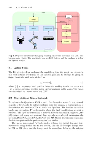
![Deep RL Applied to a Robotic Pick-and-Place Application 257
2
2
4
x
2
2
4
conv
1
1
2
x
1
1
2
conv
5
6
x
5
6
conv
2
8
x
2
8
conv
1
4
x
1
4
conv
1024
7
x
7
conv
2
2
4
x
2
2
4
conv
1
1
2
x
1
1
2
conv
5
6
x
5
6
conv
2
8
x
2
8
conv
1
4
x
1
4
conv
1024
7
x
7
conv
2048
7
x
7
concat+norm+relu
64
7
x
7
norm+conv+relu
n
7
x
7
norm+conv
n
1
1
2
x
1
1
2
upsample
Fig. 3. The CNN architecture for the action space Sa, the two main blocks are a
simplified representation of pre-trained Densenet model [25], only the feature size is
represented. The features from the Densenet model are concatenated and used to feed
the next CNN, the result is an array with Q-values used to determine the action.
dataset mean and standard deviation [26]. In general this limits the working area
of the algorithm to an approximately square area (Fig. 3).
3.3 Simulation Environment
The simulation environment was built on Webots, an open-source robotics sim-
ulator [27]. The choice has been made considering the usability of the software
and use of computational resources [28]. To enclose the simulation in the ROS
environment some modules were implemented: Gripper Control, Camera Con-
trol and a Supervisor to control the simulation. The simulated UR3e robot is
connected to ROS using the ROS driver provided by the manufacturer and con-
trolled with the Kinematics module. Figure 4 shows the simulation environment,
in which the camera is located in front of the robot, pointing to the working
area. A feature of the simulated environment is to have control over all objects
positions and colors. The positions were used as information for the reward and
the color of the table was changed randomly at each episode to increase robust-
ness during training. For each attempt the table color, the number of objects
and the position of the objects were randomly changed.
Webots Gripper Control. The Gripper Control is responsible to read and
control the position of the joints of the simulated gripper. It controls all joints,
motors and sensors of the simulated gripper. Touch sensors were also added at
the tip of the finger to emulate the feedback signal when an object is grasped.](https://image.slidesharecdn.com/optimizationlearningalgorithmsandapplications-231204021346-9e8015c0/85/Optimization-Learning-Algorithms-and-Applications-pdf-269-320.jpg)
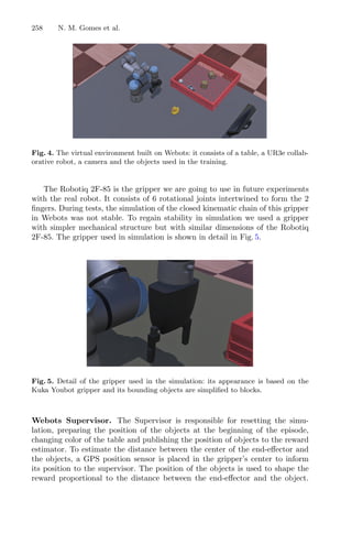
![Deep RL Applied to a Robotic Pick-and-Place Application 259
Although this information is not available in the real world they are used to
speed up the simulation training sessions.
Webots Camera. The camera simulated in Webots has the same resolution
of the Intel RealSense camera. To avoid the need of calibration of the depth
camera, both RGB and depth cameras had coincident position and field of view
in simulation. The field of view is the same as the Intel RealSense RGB camera:
69.4◦
or 1.21 rad.
3.4 Integrator
The Integrator is responsible for connecting all modules, simulated or real. It
controls the Webots simulation using the Supervisor API and feed the RGBD
images to the neural network.
Kinematics Module. The kinematics module controls the UR3e robot, simu-
lated or real. It contains several methods to execute the calculations needed for
the movement of the Cobot.
Although RL has been used to solve the kinematics in other works [22,29],
this is not the case in our system. Instead, we make use of analytical solution of
the forward and inverse kinematics of the UR3e [30]. The Denavit–Hartenberg
parameters are used to calculate forward and inverse kinematics of the robot
[31]. Considering the UR3e has 6 joints, the combination of 3 of these can give
23
= 8 different configurations which can give the same pose of the end-effector
(elbow up and down, wrist up and down, shoulder forward and back). On top
of that, the movement of the UR3e joints have a range from −2π to +2π rad,
increasing the possible solution space to 26
= 64 different configurations to the
same pose of the end-effector. To reduce the problem, the range of the joints is
limited via software to −π to +π rad, but still giving 8 possible solutions from
where the nearest solution to the current position is selected.
The kinematics module is capable of moving the robot to any position in the
work space avoiding unreachable positions. To increase the usability of the mod-
ule functions with the same behavior of the original Universal Robots “MOVEL”
and “MOVEJ” have been implemented.
To estimate the cobot joints angles in order to position the end-effector in
space the Tool Center Point (TCP) must be considered in the model. TCP is
the position of the end-effector in relation to the robot flange. The real robot
that will be used for future experiments has a Robotiq wrist camera and a 2F-85
gripper, which means that the TCP is 175.5 mm from the robot flange in the z
axis [32].
4 Results and Discussion
This section shows the results and discussion of two training sections with dif-
ferent methods. The tests were performed on a laptop with a i7-9750H CPU,](https://image.slidesharecdn.com/optimizationlearningalgorithmsandapplications-231204021346-9e8015c0/85/Optimization-Learning-Algorithms-and-Applications-pdf-271-320.jpg)
![260 N. M. Gomes et al.
32 GB RAM and a GTX 1650 4 GB GPU, running Ubuntu 18.04. Although the
GPU was not used in the CNN training, the simulation environment made use
of it.
4.1 Modules
All modules were tested individually to ensure proper functioning. The ROS
communication was tested using the builtin tool rqt , to check the connection
between nodes via topics or services. The UR3e joints positions are always pub-
lished in a topic and controlled via action client. In the simulation environment,
the camera images, the gripper control and the supervisor commands are made
available via ROS services. Differently from ROS topics, ROS services only trans-
mit data when queried, decreasing the processing demanded by Webots. Figure 6
shows the nodes via topics in the simulated environment, services are not rep-
resented in this diagram. The diagram was created with rqt .
Fig. 6. Diagram of the nodes running during the testing phase. In the simulated envi-
ronment most of the data is transmitted via ROS services. In the picture, the topics
/follow joint trajectory and /gripper status are responsible for the robot movement
and griper status information exchange, respectively.
CNN. From the four models tested, DenseNet and ResNext demanded more
memory than the available GPU while MobileNet and MNASNet were capable
of running on the GPU. To keep the fairness of the evaluation all timing tests
were performed on the CPU.
4.2 Training
For training the CNN it was used a Huber loss error function [33] and an Adam
optimizer [34] with weight decay regularization [35], the hyperparameters used
for RL and CNN training are shown in the Table 1.](https://image.slidesharecdn.com/optimizationlearningalgorithmsandapplications-231204021346-9e8015c0/85/Optimization-Learning-Algorithms-and-Applications-pdf-272-320.jpg)
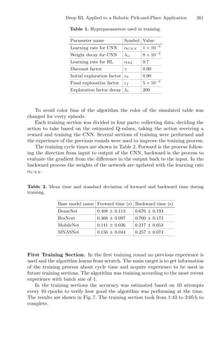
![262 N. M. Gomes et al.
In Fig. 7 is observed a training problem where the loss reaches zero and there
is no gradient for learning. The algorithm cannot learn and the accuracy shows
the q-values estimated are poor. There are several causes that can explain this
case including the weights of the CNN are too small and the experience accumu-
lated has most errors. The solutions for this are complex including fine-tuning
hyperparameters and selecting best experiences for the algorithm as shown in
[36]. Another solution is to use demonstration through shaping [37], where the
reward function is used to generate training data based on demonstrations of the
correct action to take. The training data for the second section was generated
using the reward function to map all possible rewards of the input.
Fig. 7. The loss and accuracy of 1000 epochs training section, loss data were smoothed
using a third order filter, raw data is shown in light colors.
Fig. 8. The loss and accuracy during 250 epochs training section, data were smoothed
using a third order filter, raw data is shown in light colors.
Second Training Section. The second training section used the demonstra-
tion through shaping. It was possible because in the simulation environment
the information of the position of the objects is available. The training process
received experiences generated from the simulation, these experiences have the
best action possible for each episode.](https://image.slidesharecdn.com/optimizationlearningalgorithmsandapplications-231204021346-9e8015c0/85/Optimization-Learning-Algorithms-and-Applications-pdf-274-320.jpg)


![An IoT Approach for Animals Tracking
Matheus Zorawski1(B)
, Thadeu Brito1,4,5
, José Castro2
,
João Paulo Castro3
, Marina Castro3
, and José Lima1,4
1
Research Centre in Digitalization and Intelligent Robotics (CeDRI), Instituto
Politécnico de Bragança, Campus de Santa Apolónia, 5300-253 Bragança, Portugal
{matheuszorawski,brito,jllima}@ipb.pt
2
Instituto Politécnico de Bragança, Bragança, Portugal
mzecast@ipb.pt
3
Centro de Investigação de Montanha, Instituto Politécnico de Bragança,
Campus de Santa Apolónia, Bragança, Portugal
{jpmc,marina.castro}@ipb.pt
4
INESC-TEC - INESC Technology and Science, Porto, Portugal
5
Faculty of Engineering of University of Porto, Porto, Portugal
Abstract. Pastoral activities bring several benefits to the ecosystem
and rural communities. These activities are already carried out daily with
goats, cows and sheep in Portugal. Still, they could be better applied to
take advantage of their benefits. Most of these pastoral ecosystem ser-
vices are not remunerated, indicating a lack of making these activities
more attractive to bring returns to shepherds, breeders and landowners.
The monitoring of these activities provides data to value these services,
besides being able to indicate directly to the shepherds’ routes to drive
their flocks and the respective return. There are devices in the market
that perform this monitoring, but they are not adaptable to the circum-
stances and challenges required in the Northeast of Portugal. This work
addresses a system to perform animals tracking, and the development of
a test platform, through long-range technologies for transmission using
LoRaWAN architecture. The results demonstrated the use of LoRaWAN
in tracking services, allowing to conclude about the viability of the pro-
posed methodology and the direction for future works.
Keywords: Animals tracking · IoT · GPS · Grazing monitoring ·
LoRaWAN
1 Introduction
According to breeder organizations, nearly 100.000 indigenous cows, sheep, and
goats graze daily on Portugal’s northeast rangelands. Pastoralism is widely con-
sidered to have a critical role in strengthening rural communities’ resilience and
sustainability to face depopulation and climate change [1]. Every day, hundreds
Supported by FEDER (Fundo Europeu de Desenvolvimento Regional).
c
Springer Nature Switzerland AG 2021
A. I. Pereira et al. (Eds.): OL2A 2021, CCIS 1488, pp. 269–280, 2021.
https://doi.org/10.1007/978-3-030-91885-9_19](https://image.slidesharecdn.com/optimizationlearningalgorithmsandapplications-231204021346-9e8015c0/85/Optimization-Learning-Algorithms-and-Applications-pdf-279-320.jpg)
![270 M. Zorawski et al.
of shepherds drive their flocks of 200 or fewer through multiple-ownership, small-
patched, and intricate rangelands around the farmstead [2]. Thanks to them,
natural vegetation and agricultural remnants yield excellent ecosystem services
like providing high-quality and protein-rich food, reducing fire hazards, recy-
cling organic matter, and strengthening rural communities’ identities and sense
of belonging [3,4]. Although herders are among the most impoverished peo-
ple, most of these pastoral ecosystem services are not remunerated. How can
shepherds, breeders, and landowners receive fair returns from such complicated
structures? Due to assessment objections, decision-makers struggle to regulate
and implement a payment system requiring information on multiple vegetation
changes, various grazing pressures, different species, flock sizes, duration, and
seasons.
The IPB team addresses this challenge using 30 years of joint research on tra-
ditional grazing systems in Trás-os-Montes [2]. They have demonstrated exper-
tise in updating and providing high-precision remote sensing techniques and
interpretation modeling methodologies adapted to handling large amounts of
dynamic data [4,5]. As part of its innovation and demonstration activity, the
IPB team’s projects run ten experimental sites grazed by sheep, goats, cows,
and donkeys monitored by Global Navigation Satellite System (GNSS) collars.
The team has learned the herds’ routes and routines and can accurately describe
their land and vegetation pressure. Thus, how different herds seasonally modify
the vegetation through unique pressures is the focus [2,4]. However, the IPB
team’s developments have encountered constraints in using devices and systems
available in the market, which could be applied in different contexts, purposes
and be aimed at the circumstances of the roaming pastoralism in the Northeast
of Portugal. As an example, the approach adopted by the IPB team uses col-
lars with data transmission via the Global System for Mobile (GSM) network
to track these animals. Unfortunately, this technology has a high energy con-
sumption (causing a low battery autonomy and reduced data rate), requires a
contract with telecommunications companies (which increases the project costs),
besides not being an open device for modifications and additions of new tools
(such as sensors) according to the object to be used.
A grazing monitoring system tailored to local circumstances requires
increased capabilities to record and transmit geolocations from remote sites,
with high frequency, self power supplied, and low priced. Based on continuous
feedback from the stakeholders supporting the IPB team—breeder’s organiza-
tions, Ministry of Agriculture, and the National Agency for Forest Fires—this
paper is a part of the development of such a system through the development of a
tracking and monitoring system that can be attached to the animal and provide
its behavior, i.e. perform the digitalization process. It is desired to keep the his-
tory of movements for each animal so that it is possible to analyze and use this
information further, for example, with a correlation or estimation algorithm. The
GPS position, temperature and humidity are variables that are being measured,
but the proposed system is open and ready to include new ones. This paper
presents an architecture of an Internet of Thing (IoT) approach to track animals
(based on their position) and acquire environmental conditions. As results, the](https://image.slidesharecdn.com/optimizationlearningalgorithmsandapplications-231204021346-9e8015c0/85/Optimization-Learning-Algorithms-and-Applications-pdf-280-320.jpg)
![An IoT Approach for Animals Tracking 271
acquisition, transmission, storage and visualization of the data allow validating
the proposed approach.
The rest of the paper is organized as follows: After this introduction section,
the related works compilation is presented where similar approaches are applied.
Then, Sect. 3 presents the system description where the data acquisition, trans-
mission, storage and visualization are stressed. Section 4 presents the develop-
ments and results. Last section concludes the paper and points out future work
direction.
2 Related Work
Tracking animals is a process that brings several advantages, and it was
addressed several years ago. On the one hand, different groups of researchers
are developing personalized applications, from the large scale animals to the
smallest ones [6], such as bees [7]. On the other hand, the are several commer-
cial solutions that fit this methodology but bring some disadvantages such as
the price, the closed architecture and the dependency. The animals tracking is
vital in several ways, as examples from the territory planning to the understand-
ing the predators [8]. There is also the socio-cultural and economic value of the
ecosystems [3]. Another point to monitor is the movements of flocks that bring
on different grazing pressure over the landscape [4] and also the seasonality of
grazing itineraries [2]. Another justification for the animal tracking is related to
the equilibrium of ecological dynamics on rangelands [1]. So, in the last years,
several technologies have been applied to animal tracking and behavior monitor.
Tracking animals over the cellular network is such expansive (it is necessary to
contract a company to support the communications) and, in some cases, imprac-
tical because the high energy consumption results in recurrent maintenance and
a network coverage dependency.
The fourth Industry revolution brought methodologies than can be used for
this purpose. One of them is the IoT, Internet of Things. Authors from [5]
presents an animal behavior monitoring platform, based on IoT technologies
that includes an IoT local network to gather data from animals to autonomously
shepherd ovine within vineyard areas. In this case, the data is stored on a cloud
platform, with processing capability based on a machine learning algorithm that
allows to extract relevant information. Regarding the network connections, IoT
also brought new approaches of low power networks to be applied in this filed:
examples are the LoRa and Sigfox, among others. Authors of [9] proposes a
novel design of a mesh network formed by LoRa based animal collars or tags,
for tracking location and monitoring other factors via sensors over very wide
areas. Different communication technologies can be found on [10] where collars
are connected to a Low Power Wide Area network (LPWA) Sigfox network and
low cost Bluetooth Low Energy (BLE) tags connected to those collars. From
the commercial side, has appeared a huge number of solution that may fit the
animal tracking. Some examples are the milsar™ [11] and the digitanimal™ [12].
There are also organizations that shares in a free way, the database of worldwide](https://image.slidesharecdn.com/optimizationlearningalgorithmsandapplications-231204021346-9e8015c0/85/Optimization-Learning-Algorithms-and-Applications-pdf-281-320.jpg)
![272 M. Zorawski et al.
animal tracking data, such as the movebank™ [13] hosted by the Max Planck
Institute of Animal Behavior where it is possible to researchers to manage, share,
protect, analyze and archive animal data.
Based on this study, the presented paper presents a developed solution to
track animals while monitoring the behavior. The data is collected and stored
on InfluxDB, where adaptive algorithms can be used to get precise information.
Developing a personalized application owns the advantage of including the char-
acteristics that the team desire. As a modular approach, other sensors can be
added to the system.
3 System Description
Being the main objective of this work the monitoring of pastoral activities, the
basic architecture of the system can be simplified as shown in Fig. 1, in which
the accomplishment of these steps (the first is the acquisition of coordinates in
the monitoring module, second is the transmission of these data and third is the
visualization in a platform) can be approached in several ways.
Fig. 1. System description.
Before defining which method and tools will be used to achieve the desired
system, one must verify the main needs of the project and which architecture
should be used. As this project aims to monitor automatically (not to depend
on the action of the shepherd) and with a real-time display of data in multiple
devices, it was decided to use a collar as the monitoring device and the signal
receiver to be connected to the Internet, for the storage and display not be
exclusive to the local node. Thus, Fig. 2 describes how the system architecture
should be, adding the requirements of this project.
With the system requirements defined, the following points must take into
consideration the feasibility and the restrictions of this architecture to choose
which method and strategy will be addressed, and consequently, which tools will
be used. As the Open2 project works with animal monitoring, it is essential to
be a wireless device, which implies the use of batteries, and consequently, that
it has low power consumption. Another critical point for the project is the low
cost of the entire system, seeking to create the tools and use free applications.](https://image.slidesharecdn.com/optimizationlearningalgorithmsandapplications-231204021346-9e8015c0/85/Optimization-Learning-Algorithms-and-Applications-pdf-282-320.jpg)
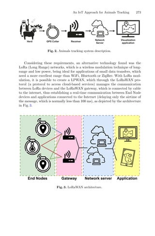
![276 M. Zorawski et al.
Fig. 6. Components used for the initial tests.
Node-RED to track the LoRa device in real-time, show path travelled, store data
locally in the .log file in the InfluxDB database. This flow can be applied in
multiples devices, allowing the storage and display of registered TTN devices.
Fig. 7. Flow used to track the LoRa device.
After implementing the Node-RED and verifying the system’s operation to
better acquire the coordinates and trajectories, the End Node was replaced by
a device capable of wireless data transmission. For this it was used the Printed
Circuit Board (PCB) of the SAFe project [14–17] (shown in Fig. 8), which already
contained part of the architecture presented in Fig. 4, with a DHT sensor module,
powered by a battery and protected by a 3D printed box, only needing to add the
GPS module. The temperature and humidity sensor (DTH11) was used when
sent the payload, but has not been applied in the following visualization steps.](https://image.slidesharecdn.com/optimizationlearningalgorithmsandapplications-231204021346-9e8015c0/85/Optimization-Learning-Algorithms-and-Applications-pdf-286-320.jpg)
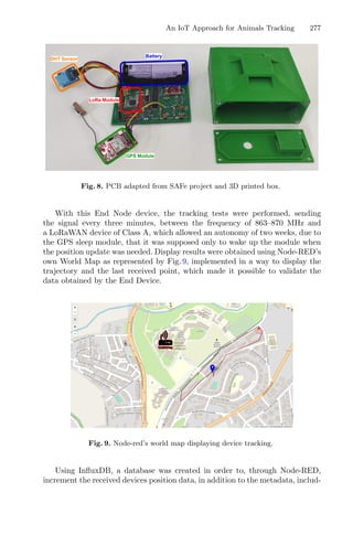

![282 T. Brito et al.
council). These alerts will be parameterized and presented in a personalised way
and tailored to each actor. Thus, it is intended to minimise the occurrence of
ignitions, monitor fauna and flora, and contribute to the environmental develop-
ment of the region of Trás-os-Montes, particularly in the district of Bragança. In
addition to the capacity for early detection of forest fires, the accurate estimation
of the fire hazard, using fire risk indices in real-time, on a sub-daily and local
scale, in meteorological data, in the availability of fuels and moisture content
vegetation is of utmost importance.
The SAFe’s implementation is localised to the Serra da Nogueira area, belong-
ing to the Natura 2000 Network, with unique characteristics in the Bragança
region and with an extension of approximately 13 km. Considering the region’s
size to be monitored, data transmission is carried out by LoRaWAN, it is based
on low power wide area network, which will guarantee full coverage of the area
in question [1–4]. This type of communication is increasingly used, and it is
estimated that by 2024, the IoT industry will generate revenue of 4.3 trillion
dollars [5]. LoRaWAN networks are composed of end devices, gateway and net-
work server in the midst of a rising state. The data is acquired from the modules
(end devices) that send the data to the gateway, which in turn relays the mes-
sages to the servers through non-LoRaWAN networks, such as Ethernet or IP
over cellular [6].
The LoRaWAN communication itself uses the Chirp Spread Spectrum (CSS)
modulation, where chirp pulses modulate the signal. It uses an unlicensed sub-
gigahertz ISM band that varies in width depending on the region of application,
and for Europe, it is 863 MHz to 870 MHz [7]. Within the communication set-
tings, three parameters allow a network adjustment between bit rate and robust-
ness of the transmission: Bandwidth (BW), Spreading Factor (SF), and Coding
Rate (CR) [8]. The format of the Long Range (LoRa) message is subdivided into
several layers, the physical layer, which is composed of five fields, the pream-
ble, the physical header (PHDR), the physical header Cyclic Redundancy check
(PHDR0 CRC), the physical payload (PHY Payload) and an error detection tail
(CRC). The Medium Access Control (MAC) layer, in turn, is a subdivision of
the PHY Payload field and consists of three fields, the MAC Header (MHDR),
MAC Payload and the Massage Integrity Code (MIC). Within the MAC Payload
is the message itself, which consists of three fields, the Frame header (FHDR),
the port and the frame payload (FRM Payload) [9].
At this stage of the SAFe project, while the testing period is still underway in
an urban environment, the configuration being used is a 125 kHz Bandwidth, an
SF7 and a Coding Rate of 4/5, which allows transmission of about 242 Bytes.
However, taking into account that when the project passes the test phase in
a rural environment, it will be necessary to cover a larger area. It is probably
required to use a larger SF to improve the communication range, thus reducing
transmission capacity. Using an SF12 and maintaining the BW and CR, the
LoRaWAN communication will allow transmission of about 51 Bytes. Therefore,
there is a necessity to optimise the use of all bits’ packages as much as possible
and not lose data essential for the project’s realisation. But some sensors have](https://image.slidesharecdn.com/optimizationlearningalgorithmsandapplications-231204021346-9e8015c0/85/Optimization-Learning-Algorithms-and-Applications-pdf-292-320.jpg)
![Optimizing Data Transmission in a Wireless Sensor Network 283
a 10 or 12 bits resolution while LoRaWAN owns 8 bits, which means, in some
cases, multiples slots of transmission remaining unused bits. In this way, this
paper addresses a communication optimisation for Wireless Sensors Network
(WSN) resorting to encoding and decoding procedures.
The rest of paper is organized as follows. After the introduction, Sect. 2
presents the related work. In Sect. 3, the system architecture is addressed where
the focus of this paper is highlighted. Section 4 presents the algorithm used to
optimise the data sent though the network and Sect. 5 stresses the results of
the proposed encoding/decoding. Last section, concludes the paper and points
future work.
2 Related Work
Real-time data collection and analysis had new possibilities with the emergence
of the Internet of Things (IoT). Typically, IoT devices are manufactured to use in
short-range protocols, such as Bluetooth, WiFi, and ZigBee, among others, which
may have limitations, such as the maximum number of devices connected to the
gateway and high power consumption. On the other hand, mobile technologies
that have an extensive range (LTE, 3G and 4G) are expensive, consume a lot of
power and have a continuing cost [10]. The gap that these technologies have been
filled in part by Low Power Wide Area Network (LPWAN) technologies, which
cannot cover the critical applications (e.g. remote health monitoring), but fit
very well for the requirements of IoT applications. Although low data rates limit
LPWAN systems, there are reasons for their use, especially after the emergence
of technologies such as SigFox, NB-IoT, and LoRa [10,11].
LoRa network is highly used in applications requiring low power consumption
and long-range, in which LoRa Alliance proposed the LoRaWAN, defining the
network protocol in the MAC and network layers [10,12]. Different scenarios of
typical LoRa networks applications are pointed out in [12], besides providing
documentation of LoRa networks design and implementation, searching for a
better cost-benefit for LPWAN applications. Also, Baiji [13] showed in 2019 an
application using LoRaWAN in an IoT monitoring system aimed to minimise
the non-productive time for Oil and Gas companies through the detection of a
leak.
Researches are being carried out seeking improvements to the LoRaWAN
system, in which numerous of these are being carried out to seek optimisa-
tion of data rate, airtime, and energy consumption through an Adaptive Data
Rate (ADR), as in [14], where a review of research on ADR algorithms for
LoRaWAN technology is presented. Also, in [15] a method for the use of ADR is
implemented, seeking to provides an optimal throughput with multiple devices
connected to LoRaWAN. Furthermore, a study was carried out looking for max-
imising the battery lifetime through different LoRaWAN nodes and scenarios in
[16], demonstrating relationships between different payload sizes with the power](https://image.slidesharecdn.com/optimizationlearningalgorithmsandapplications-231204021346-9e8015c0/85/Optimization-Learning-Algorithms-and-Applications-pdf-293-320.jpg)
![284 T. Brito et al.
consumption and air time using various SF and CR, indicating an increase in
power consumed per bit of payload used.
As cited by [11], all the advantages of the LoRa network of achieving a long
transmission range, low power and enabling low-cost IoT applications to exist
with the downside of low data throughput rate. The LoRaWAN data transfer
must respect a protocol, and it is possible to send the Payload in several forms,
as long as it is within the limit of the number of Bytes. Considering the article
[9], the LoRa message format is composed of several fields that have specific or
limited sizes. Therefore, it is necessary to optimise the use of bytes in Payload
as much as possible. Some techniques have been used over the years, such as
selecting the best packet size by adjusting the bit rate to achieve maximum
throughput as demonstrated by the authors of the article [17], to optimise the
payload sizes in voice and video applications. Still, within this dynamic, the
authors of the article [18] used throughput as the optimisation metric and based
their study on wireless ATM networks to maximise the efficiency of transfer
by adapting the packet size with the variation of the channel conditions. Also,
Eytan Modiano in [19] presented a system to dynamically optimise the packet
size based on the estimates of the channel’s bit error rate, being particularly
useful for wireless and satellite channels.
The importance of packet size optimisation in WSN are debated in the article
[20], presenting several packet size optimisation techniques and concluding that
there is no agreement on whether the packet should be fixed or dynamic. The
packet size optimisation technique to be used for WSN is defended in article
[21], proposing an energy efficiency factor evaluation metric, being a fixed packet
size for the case studied. Furthermore, the authors of the article [22] present a
variation of the packet size depending on the network conditions to increase the
network throughput and efficiency. The method of payload recommended by The
Things Network (TTN) when using LoRaWAN has described in [23] only the
specifications of how to send each type of data. Suppose the user needs to use
the minimum Bytes possible for a shorter transmission time and being within
the limit of 51 Bytes. One way to implement data encoding for the LPWAN
network as LoRaWAN is through Cayenne Low Power Payload (LPP), which
allows sending the payload dynamically, according to the LoRa frequency and
data rate used [24]. Nevertheless, besides the various optimisations that have
been mentioned above, it remains crucial to find the form to optimise the data
that will be transferred for better use of the LoRa network.
3 System Architecture
The presented system has the main ideology of monitoring a determined area
with a reduced application cost. In this way, it is expected to obtain constant
surveillance to identify any ignition that may exist. This surveillance will be
achieved using the various sensors present in the modules (end devices). Each
module consists of six sensors, with three distinct values types: five flame sensors
and a sensor that provides data on relative humidity and air temperature. The](https://image.slidesharecdn.com/optimizationlearningalgorithmsandapplications-231204021346-9e8015c0/85/Optimization-Learning-Algorithms-and-Applications-pdf-294-320.jpg)
![Optimizing Data Transmission in a Wireless Sensor Network 285
entire operation of the safe project combines the collection of data from the
modules present in the forest; this data collection mustn’t fail. Consequently, the
proper functioning of data transmission is guaranteed because if the data does
not reach the competent entities, they will be of no use. This transmission will be
handle using LoRaWAN technology, which allows us to connect several modules
to different gateways. Thus, guaranteeing low-cost and efficient coverage of the
area. Figure 1 exemplifies the whole system architecture of the SAFe project.
Fig. 1. System architecture of SAFe project [2].
Due to the specificity that each of these elements is defined and developed
(Fig. 1), this work is concentrated only on the LoRaWAN’s Transmission and
the proposed arrangement bits protocol. Other SAFe’s approaches can be seen
in [1–4]. In this way, considering the high number of modules (end devices)
used in this project, there is a requirement to ensure no collisions between their
messages; the whole modules’ description is explained in [2,4]. Thereupon, it is
necessary to optimise the size of the data package sent, thus guaranteeing the
minimum necessary occupation of bytes to reduce the chances of these collisions
and consequent data losses. The normal sending process (recommended by TTN
service) will be exemplified below to explain the process, for this information will
be used related to the six sensors present in the modules as well as the battery
information, resulting in:](https://image.slidesharecdn.com/optimizationlearningalgorithmsandapplications-231204021346-9e8015c0/85/Optimization-Learning-Algorithms-and-Applications-pdf-295-320.jpg)
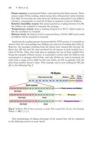
![Optimizing Data Transmission in a Wireless Sensor Network 287
4 Algorithm
From the previous section, it is possible to notice that for each flame sensor data
(S[i]), there are some unused bits (x) available to receive data to be carried.
In this way, the humidity sensor (RH) and the temperature sensor (T) will be
stored on a Byte type and the battery (B) level will be stored in 10 bits reso-
lution. Table 1 presents the transmission package without optimise the encoding
procedure (using the recommendation in [23]).
Table 1. Transmission without optimise encoding. S[i] are the flame sensors, H, T and
B are the Humidity, Temperature and Battery Voltage sensors, respectively. The ‘x’
are the unused bits.
S[0] RH
x x x x x x s9[0] s8[0] ... s0[0] x x x x x x x RH7 ... RH0
S[1] T
x x x x x x s9[1] s8[1] ... s0[1] x x x x x x x T7 ... T0
S[2] B
x x x x x x s9[2] s8[2] ... s0[2] x x x x x x B9 B8 ... B0
S[3] Legend
x x x x x x s9[3] s8[3] ... s0[3] Used by 10 bits sensors
Used by Relative Humidity
S[4] Used by Temperature
x x x x x x s9[4] s8[4] ... s0[4]
This approach intends to sort the bits using a less value as possible in bytes
protocol used to transmit the data by LoRaWAN. The main idea is distribute
each bit from each sensor during the encoding process, in a manner that is
necessary use the minimum Bytes. In order to optimise these Not Used bits (b15,
b14, b13, b12, b11 and b10, see Fig. 2) for each sensor S[i] (where i ∈ R|0 ≤ i ≤
4), the word (2-Bytes) of Humidity (RH), Temperature (T) and Battery (B) will
be separated and combined with the unused bits at the encoding procedure. A
bit manipulation operation is required to use the previous unused bits. Table 2
presents the previous “x” assuming bits from other sensors. Moreover, even
including the H, T and B values, there are 4 bits that remains unused. They will
be appropriated to hold four auxiliary bits (AUX) for future applications.](https://image.slidesharecdn.com/optimizationlearningalgorithmsandapplications-231204021346-9e8015c0/85/Optimization-Learning-Algorithms-and-Applications-pdf-297-320.jpg)
![288 T. Brito et al.
Table 2. Proposed encoding map.
S[0] RH
T5 T4 T3 T2 T1 T0 s9[0] s8[0] ... s0[0] x x x x x x x x ... x
S[1] T
RH3 RH2 RH1 RH0 T7 T6 s9[1] s8[1] ... s0[1] x x x x x x x x ... x
S[2] B
B1 B0 RH7 RH6 RH5 RH4 s9[2] s8[2] ... s0[2] x x x x x x x x ... x
S[3] Legend
B7 B6 B5 B4 B3 B2 s9[3] s8[3] ... s0[3] Used by 10 bits sensors
Used by Relative Humidity
S[4] Used by Temperature
AUX4 AUX2 AUX1 AUX0 B9 B8 s9[4] s8[4] ... s0[4] Used by AUX
This encoding operation is carried by an embedded system that is pro-
grammed on C language. For the encoding, the proposed C code is detailed
on Listing 1.1. The message will go through the network and will be decoded by
Listing 1.2.
Listing 1.1. Data encoder
S [ 0 ] = S [ 0 ] + (T 0X3F) 10;
S [ 1 ] = S [ 1 ] + (T 0XC0) 10 + (H 0X0F) 12;
S [ 2 ] = S [ 2 ] + (H 0XF0) 10 + (B 0X003) 14;
S [ 3 ] = S [ 3 ] + (B 0X0FC) 10;
S [ 4 ] = S [ 4 ] + (B 0X300) 10 + (AUX 0X0F) 12;
//TRANSMIT array S
An opposite operation of decoding will allow to extract the Flame values,
Humidity, Temperature and Battery voltage from the message. The C code of
decoding procedure can be found on Listing 1.2.
Listing 1.2. Data decoder
//RECEIVE array S
T = (S [ 0 ] 0XFC00) 10 + (S [ 1 ] 0X0C0) 4;
H = (S [ 1 ] 0XF000) 12 + (S [ 2 ] 0X3C00) 6;
B = (S [ 2 ] 0XC000) 14 + (S [ 3 ] 0XFC00) 10
+ (S [ 4 ] 0X0C00) 2;
AUX = (S [ 4 ] 0XF000) 12;
S [ 0 ] = S [ 0 ] 0X03FF ;
S [ 1 ] = S [ 1 ] 0X03FF ;
S [ 2 ] = S [ 2 ] 0X03FF ;
S [ 3 ] = S [ 3 ] 0X03FF ;
S [ 4 ] = S [ 4 ] 0X03FF ;](https://image.slidesharecdn.com/optimizationlearningalgorithmsandapplications-231204021346-9e8015c0/85/Optimization-Learning-Algorithms-and-Applications-pdf-298-320.jpg)
![Optimizing Data Transmission in a Wireless Sensor Network 289
This optimised message can be sent to the LoRaWAN network and at the
destination, a decoder procedure will construct the original message. Figure 3
presents the encoding, transmission and decoding procedures. As it can be seen,
the packet to be sent keeps the size of produced by the flame sensors S[i] (where
i ∈ R|0 ≤ i ≤ 4):
Fig. 3. Encoding and decoding procedures. Size of S[i] is 16 bits whereas T and H are
8 bits. AUX is an auxiliary variable that was created with the 4 bits that remain free.
By this way, a reduction of transmission from 8 words (16-Bytes) to 5
words (10-Bytes) is obtained. The following section demonstrates the difference
between the procedure of recommendation by TTN and this approach.
5 Results
To demonstrate the difference during transmission using the LoRaWAN network
with the algorithm proposed in this work, a comparison test is performed with
the method recommended by TTN. Therefore, five sensor modules are config-
ured for each transmission method: five nodes with the TTN transmission tech-
nique and another five nodes with the algorithm shown in the previous section.
Figure 4a shows the ten modules distributed on the laboratory bench. They are
configured according to the mentioned algorithms and simulate a small WSN.
All of these modules are configured to transmit at a specific frequency within the
range that LoRaWAN works. In this way, it is possible to probe the behaviour
of the duty cycle in the settings of the gateway used. The gateway used is RAK
7249, which is attached to the laboratory’s roof shown in Fig. 4b.](https://image.slidesharecdn.com/optimizationlearningalgorithmsandapplications-231204021346-9e8015c0/85/Optimization-Learning-Algorithms-and-Applications-pdf-299-320.jpg)
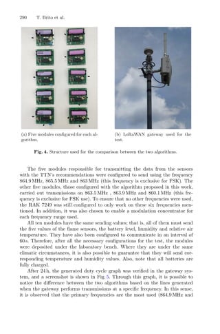
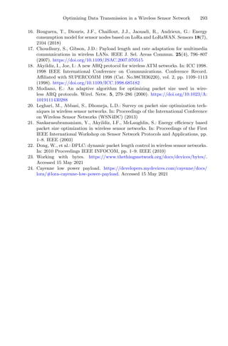
![Indoor Location Estimation 295
The beacon-based solution is based on the existence of a network of receivers
or transmitters (positioning-infrastructure), some of them placed at known loca-
tions. In this solution, the location is estimated by multilateration [1] (or tri-
angulation for angles) from a set of measured ranges. These methods are also
named Indoor Positioning Systems (IPS), depending on the sensor configura-
tion and processing approach, using technologies such as ultrasound, middle to
short-range radio (Wi-Fi, Bluetooth, UWB, RFID, Zigbee, etc.) or vision [2]. The
main weakness of these solutions is the need for infrastructure, limited absolute
accuracy and coverage.
The beacon-free solution, mainly relying on dead-reckoning methods with
sensors installed on the target to be located, uses Inertial Measuring Units (IMU)
and odometry to estimate the position of the target [3]. They integrate step
lengths and heading angles at each detected step [4] or, alternatively, data from
accelerometers and gyroscopes [5,6]. IMU and odometry based location have
the inconvenience of accumulating errors that drift the path length.
Beacon-based solutions using short-range radio signals deduce the distance by
measuring the received signal strength (RSS), mainly based on two methods: i)
the use of a radio map (previously established or online measured) as a reference;
or, ii) the use of probabilistic methods such as Bayesian inference to estimate
the location of the target.
The implementation of beacon-based solutions requires the existence of a
positioning-infrastructure. While it is possible to achieve extremely high accu-
racy with a specific ad-hoc positioning-infrastructure, the cost of installing and
maintaining the required hardware is a significant drawback of such systems.
On the contrary, the use of an existing beacon-based network (such as Wi-Fi or
Bluetooth) as a non-dedicated positioning-infrastructure could require no extra
hardware installation and minimal adjustments in software to implement an IPS,
but, it typically results in lower accuracy [7–9]. Therefore, most of the research
lines for non-dedicated positioning-infrastructures are focused on increasing the
accuracy in location estimation by using curve fitting and location search in
subareas [9], along with different heuristic-based or mathematical techniques
[10–12].
In this work, a low complexity positioning solution based on an existing
Wi-Fi infrastructure is proposed. Such technology is extremely wide extended
and allowable, therefore it is easily scaled to fill coverage gaps with inexpensive
devices. One of them is the ESP8266 board, made by Espressif Systems, which
has a low-cost Wi-Fi microchip and meandered inverted-F PCB antenna, with
a full TCP/IP stack and a microcontroller.
This solution includes a collaborative node strategy by processing fixed and
dynamic information depending on the environment status, holding the line
started by other authors [13,14] and improving the broadcasting method with
new results [15]. In addition, it assumes no prior knowledge of the statistical
parameters that represents the availability of the RF channel, it can also dynam-
ically adapt to variations of these parameters.](https://image.slidesharecdn.com/optimizationlearningalgorithmsandapplications-231204021346-9e8015c0/85/Optimization-Learning-Algorithms-and-Applications-pdf-305-320.jpg)
![296 A. Mendes and M. Diaz-Cacho
Additionally, the solution has low computational complexity and low energy
consumption, which makes it attractive to be implemented in vehicles, mobile
robots, embedded and portable devices and, especially, in smartphones.
However, there are several issues with this type of location mechanism. Inher-
ent in all signal measurement exists a degree of uncertainty with many sources
(interferences, RF propagation, location of the receiver, obstacles in the path
between transmitter and receiver, etc.). This uncertainty could have a signifi-
cant effect on the measured RSS values, and therefore on the accuracy of the
received signal. In addition, because of the RF wave propagation characteristics
within buildings, the RSS values themselves are not a uniform square law func-
tion of distance. This means that a particular RSS value may be a close match
for more than one RF transmission model curve, pointing that some dynamic
adjustment may be necessary from time to time.
Moreover, some contributions could be stated, as early simulations yield aver-
age location errors below 2 m in the presence of both range and interference
location inaccuracies, experimentally confirmed afterwards; well-performed in
real experiments compared with some related mechanism from the literature;
use COTS inexpensive and easy to use hardware being beacon devices; verify
the barely intuitive idea that there is a trade-off between the number of beacon
devices and the location accuracy.
The paper is organized as follows. This section presented the concept, moti-
vation and common problems of indoor positioning technologies, and in addition
an introduction to the proposed solution. Section 2 provides the basic concepts
and problems encountered when implementing positioning algorithms in non-
dedicated positioning-infrastructures and describes the system model. A novel
positioning-infrastructure based on collaborative beacon nodes is presented in
Sect. 3. Simulation and real implementation results are presented and discussed
in Sect. 4, and finally, Sect. 5 concludes the paper and lists future works.
2 System Model
In this section, we describe the system model, which serves as the basis for the
design and implementation of our proposal. This model allows determining the
location of a client device by using management frames in Wi-Fi standard [16,17]
and Received Signal Strength (RSS) algorithm combined with the lateration
technique [18,19].
Many characteristics make positioning systems work different from outdoor
to indoor [19]. Typically, indoor positioning systems require higher precision and
accuracy than that shaped for outdoor to deal with relatively small areas and
existing obstacles.
In a strict comparison, indoor environments are more complex as there are
various objects (such as walls, equipment, and people) that reflect, refract and
diffract signals and lead to multipath, high attenuation and signal scattering
problems, and also, such systems typically rely on non-line of sight (NLoS) prop-
agation where the signal can not travel directly in a straight path from an emitter
to a receiver, which causes inconsistent time delays at the receiver.](https://image.slidesharecdn.com/optimizationlearningalgorithmsandapplications-231204021346-9e8015c0/85/Optimization-Learning-Algorithms-and-Applications-pdf-306-320.jpg)
![Indoor Location Estimation 297
On the other hand, there are some favourable aspects [19], as small coverage
area becomes relatively under control in terms of infrastructure, corridors, entries
and exits, temperature and humidity gradients, and air circulation. Also, the
indoor environment is less dynamic due to slower-speed moving inside.
Lateration (trilateration or multilateration, depending on the number of ref-
erence points), also called range measurement, computes the location of a target
by measuring its distance from multiple reference points [1,16].
Fig. 1. Basic principle of the lateration technique for 2-D coordinates.
In Fig. 1, the basic principle of the lateration method for a 2-D location
measurement is shown. If the geographical coordinates (xi, yi) of, at least, three
reference elements A, B, C are known (to avoid ambiguous solutions), either
the measured distances dA, dB and dC, then the estimated position P(x̂,ŷ),
considering the measured error—grey area in figure—, can be calculated as a
solution for a system of equations that could be written similarly as Eq. 1, for
the x-axis.
dxi
=
(x̂ − xi)2 + (ŷ − yi)2 (1)
for {i ∈ Z | i 0}, where i is the number of reference elements.
In our model, we consider a static environment with random and grid deploy-
ments of S sensor nodes (throughout this work called only as nodes), which could
be of two different types:
– Reference, which can be an available Wi-Fi compliant access point (AP);
and,
– Beacon, which is made with the inexpensive Espressif ESP8266 board with
a built-in Wi-Fi microchip and meandered inverted-F PCB antenna, a full
TCP/IP stack and a microcontroller.](https://image.slidesharecdn.com/optimizationlearningalgorithmsandapplications-231204021346-9e8015c0/85/Optimization-Learning-Algorithms-and-Applications-pdf-307-320.jpg)
![298 A. Mendes and M. Diaz-Cacho
Both types are in a fixed and well-known location, but there is also a client
device that is a mobile device. All these nodes are capable of wireless communi-
cation.
The client device has installed inside a piece of software that gathers infor-
mation from those nodes and computes its proper location, by using an RF
propagation model and the lateration technique. Therefore, based on a RSS
algorithm, it can estimate distances. The RSS algorithm is developed in two
steps:
i. Converting RSS to estimated distance by the RF propagation model; and,
ii. Computing location by using estimated distances.
Remark that the RF propagation model depends on frequency, antenna ori-
entation, penetration losses through walls and floors, the effect of multipath
propagation, the interference from other signals, among many other factors [20].
In our approach, we use the Wall Attenuation Factor (WAF) model [8] for
distance estimation, described by Eq. 2:
RSS(d) = P(d0) − 10α log10( d
d0
) − WAF
×
nW, if nW C
C, if nW ⩾ C
(2)
where RSS is the received signal strength in dBm, P(d0) is the signal power
in dBm at some reference distance d0 that can either be derived empirically or
obtained from the device specifications, and d is the transmitter-receiver sepa-
ration distance. Additionally, nW is the number of obstructions (walls) between
the transmitter and the receiver and C is its maximum value up to which the
attenuation factor makes a difference, α indicates the rate at which the path
loss increases with distance, and WAF is the wall attenuation factor. In general,
these last two values depend on the building layout and construction material
and are derived empirically following procedures described in [8].
Since the environment varies significantly from place to place, the simplest
way to find the relationship of RSS and the distance between a pair of nodes is
collecting signal data at some points with known coordinates. Moreover, this is a
learning mode procedure that can improve the lateration process by the adoption
of real environment particularities, and also helps to determine empirically the
path loss exponent α.
Therefore, we determine α pruning the path loss model to a form in which it
presents a linear relationship between the predicted RSS and the logarithm of the
transmitter-receiver separation distance d, and then, we apply a linear regres-
sion to obtain that model parameter. Observe that C and nW are determined
according to the type of facility.
3 Distributed Collaborative Beacon Network
In this section, we introduce the distributed collaborative beacon network for
indoor environments.](https://image.slidesharecdn.com/optimizationlearningalgorithmsandapplications-231204021346-9e8015c0/85/Optimization-Learning-Algorithms-and-Applications-pdf-308-320.jpg)
![Indoor Location Estimation 299
Our goal is to improve the client location accuracy by enhancing the infor-
mation broadcasted by nodes.
3.1 Proposal
Unlike traditional location techniques based on Wi-Fi [17], which map out an
area of signal strengths while storing it in a database, beacon nodes are used to
transmit encoded information within a management frame (beacon frame), which
is used for passive position calculation through lateration technique. Observe
that we are focusing on the client-side, without the need to send a client device
position to anywhere, avoiding privacy concerns. Moreover, since this is a purely
client-based system, location latency is reduced compared to a server-side imple-
mentation.
To improve location accuracy, we propose a collaborative strategy where
nodes exchange information with each other. Every 5 s, during the learning
mode, a beacon node randomly (with probability depending on a threshold ε)
enters in scanning mode [16,17]. The node remains in this mode during at least
one beacon interval (approximately 100 ms) to guarantee the minimum of one
beacon received from any reference node (access point) in range.
A beacon node receives, when in learning mode, RSS and location informa-
tion from reference nodes in range, and therefore can calculate a new α value
using Eq. 2. After, the new propagation parameter (α) and the proper location
coordinates are coded and stuffed into the SSID, then broadcasted to the clients.
Reference nodes only broadcast its proper location.
It is noted that the path loss model plays an important role in improving the
quality and reliability of ranging accuracy. Therefore, it is necessary to investi-
gate it in the actual propagation environment to undermine the obstruction of
beacon node coverage (e.g. people, furniture, etc.) tackling the problem of NLoS
communication.
Once in place, this coded information allows a client device to compute
distances through lateration, then determining its proper location. All of this
is performed without the need for data connectivity as it is determined purely
with the information received in beacon frames from nodes in range.
The coding schema in the standard beacon frame (also known as beacon stuff-
ing [13]) works in nearly all standard-compliant devices and enhancing them if
multiple SSIDs are supported, thus allowing to use of an existing SSID, simul-
taneously.
Beacon frames must be sent at a minimum data rate of 1 Mbps (and standard
amendment b [16,17]) to normalize the RSS across all devices. In general, since
the RSS will change if data rate changes for management data frames, in this
way it did not get any variation in RSS on the client device, except for range.
Consideration should be made when planning the optimal placement of the
beacon nodes, but this will generally be dictated by existing infrastructure (e.g.,
if using an existent standard-compliant access point as reference node), build-
ing limitations or power source requirements.](https://image.slidesharecdn.com/optimizationlearningalgorithmsandapplications-231204021346-9e8015c0/85/Optimization-Learning-Algorithms-and-Applications-pdf-309-320.jpg)
![300 A. Mendes and M. Diaz-Cacho
Algorithm 1: BEACON node
1 Initialization of variables;
2 while (1) do
3 /* zeroing the information array */
4 /* and fill in a proper location */
5 Initialization of I[1..nodes];
6 /* check time counter */
7 if (counter % 5) then
8 draws a random number x, x ∈ [0, 1];
9 /* learning mode */
10 if (x ε) then
11 WiFi Scanning;
12 get SSID from beacon frame;
13 foreach ref node in SSID do
14 read coded information;
15 Decode;
16 get {location, RSS};
17 I[ref node] ← {location, RSS};
18 /* adjust α if needed */
19 if (α do not fit default curve) then
20 ComputeNewAlpha;
21 I[ref node] ← {α};
22 /* beacon frame coding */
23 PackAndTx ← I;
24 Broadcast coded SSID;
3.2 Algorithms and Complexity Analysis
The proposed strategy is described in Algorithms 1 and 2.
In the beginning, after initialization, the mechanism enters into an infinite
loop during its entire period of operation. And from a beacon node point of
view, it decides according to a threshold (ε) between enter in learning mode, as
described earlier or jump directly to the coding process of its proper location
coordinates into the SSID, and transmission. In Algorithm 2, a client device
verifies if a received beacon frame comes from a beacon or a reference node,
then run the routines to decode informations and adjust α, if needed, and at last
computes its location.
Finally, observing Algorithm 1, it is noted that it depends of three routines,
named Decode, ComputeNewAlpha and PackAndTX, which are finite time oper-
ations with time complexity constant, O(1). However, it all depends on the
number of reference nodes in range, this way it raises the whole complexity
to T(n) = O(n). In a similar fashion, Algorithm 2 depends on Decode and
AdjustAlpha routines, which are finite time operations, but the Positioning](https://image.slidesharecdn.com/optimizationlearningalgorithmsandapplications-231204021346-9e8015c0/85/Optimization-Learning-Algorithms-and-Applications-pdf-310-320.jpg)
![Indoor Location Estimation 301
Algorithm 2: CLIENT device
1 Initialization of variables;
2 while (1) do
3 WiFi Scanning;
4 get SSID from beacon frame;
5 foreach (ref node|beacon node in SSID) do
6 read coded information;
7 Decode;
8 AdjustAlpha;
9 Positioning;
routine takes linear time, also dependent on the amount of nodes (reference
and beacons) in range, thus the complexity becomes linear, T(n) = O(n).
Additionally, the largest resource consumption remains related to the storage
of each coded SSID (32 bytes), which is dependent on the number of nodes
(reference and beacons) in range as well. Thus, S(n) = O(n).
4 Evaluation
In this section, the proposed collaborative strategy is evaluated using numerical
simulations, also by a real implementation experiment using the inexpensive
ESP8266 board [21], a Wi-Fi standard-compliant access point and a smartphone
application software.
Location estimation is the problem of estimating the location of a client
device from a set of noisy measurements, acquired in a distributed manner by
a set of nodes. The ranging error can be defined as the difference between the
estimated distance and the actual distance.
The location accuracy of each client device is evaluated by using the root
mean square error (Eq. 3):
ei =
(x − xe)2 + (y − ye)2 (3)
where x and y denote the actual coordinates, and xe and ye represent the esti-
mated coordinates of the client.
We define the average location error (e) as the arithmetic mean of the location
accuracy, as seen in Eq. 4:
e =
N
j=1
ei
N
(4)
To assist in the evaluation, the strategies are analyzed in terms of average
location error (e), and additionally, some other metrics are used and discussed
occasionally, such as accuracy, technology, scalability, cost, privacy, and robust-
ness [16,19,22].](https://image.slidesharecdn.com/optimizationlearningalgorithmsandapplications-231204021346-9e8015c0/85/Optimization-Learning-Algorithms-and-Applications-pdf-311-320.jpg)

![304 A. Mendes and M. Diaz-Cacho
Apart from that, when looking at Fig. 3b, the average energy consumption
by our strategy is stable in comparison with other strategies. As expected, with
clients running a simplified mechanism and only beacon frames being broad-
casted by beacon nodes, our proposed approach significantly improves the resid-
ual energy of the overall network, for both scenarios.
4.2 Real Implementation Analysis
Our real implementation analysis has been made with placement around the bor-
der of a corridor that connect offices at the Department of Systems Engineering
and Automatics’ (DESA) facility, as shown in Fig. 4.
Fig. 4. DESA’s facility real scenario and heatmap overlay (beacon and reference
nodes—B and R respectively).
We deploy at least one beacon node (made with the ESP8266 board) on each
corner until 8 nodes (01 Wi-Fi standard-compliant access point included) being
placed in total, and a client device (smartphone), in an area of 200 m2
, where
the maximum distance between nodes lies between 2 m and 3 m. To avoid the
potential for strong reflection and multipath effects from the floor and ceiling,
we kept all devices away from the floor and ceiling.
The α parameter (Eq. 2) has a initial value of 2.0 and the threshold ε is set
to 0.1.
Before running the experiment, we measured received signal strengths from
each node (beacon or reference node) of our network. These measurements
were made from distances ranging between 1 m to 20 m of each node, in 10
points within the area of the experiment, totalizing 200 measurements, aided
by a smartphone application. Figure 4 shows a heat map overlay made with the
average of these measurements.
In addition, we added functions to the base firmware of the board ESP8266
(esp iot sdk v1.3.0 SDK [21]) to execute the learning process, described in Sub-
sect. 3.1.
During the experiment, on the smartphone application, the trilateration pro-
cess uses a RSS based path loss algorithm to determine the distance (Eq. 2).](https://image.slidesharecdn.com/optimizationlearningalgorithmsandapplications-231204021346-9e8015c0/85/Optimization-Learning-Algorithms-and-Applications-pdf-314-320.jpg)
![306 A. Mendes and M. Diaz-Cacho
10
20
30
40
50
60
70
80
90
100
0 2 4 6 8 10
CDF
(%)
Avg. location error (m)
Simulated
Real
(a) Our strategy: simulated vs real. (b) Benchmarking between mechanisms.
Fig. 6. Average location error (e) CDF comparison (by real experiment).
By comparing the results in Fig. 5a to the ones in Fig. 2, one can observe that
the performance of the WELO is positively impacted with the growth of the amount
of beacon nodes available, but with a limit. Additionally, the performance degra-
dation is small, which shows the robustness of the proposed strategy against the
larger heterogeneity of a real indoor scenario without any prior knowledge.
Based on the above observations, we compared the average location error (e)
CDF comparison (by real experiment) in Fig. 6. Figure 6a shows its performance
in simulations in contrast with its capabilities in the real experiments. At that,
we can observe the accuracy suffering from the toughness of the indoor scenario.
Figure 6b shows the performance evaluation of the proposed strategy against
some classical algorithms, such as RADAR [8] and Curve Fitting with RSS
[9] in the office indoor scenario, together with GNSS (worse performance and
related to upper x-axis only). As can be seen, WELO shows its suitability and
its lower average location error almost of the time within the scenario. From
these figures, WELO results are fairly stimulating and we can observe performance
improvements.
5 Conclusions
The Wi-Fi standard has established itself as a key positioning technology that
together with GNSS is widely used by devices.
Our contribution is the development of a simple and low-cost indoor loca-
tion infrastructure, plus a low complexity and passive positioning strategy that
does not require specialized hardware (instead exploiting hardware commonly
available—ESP8266 board—with enhanced functionality), arduous area polling
or reliance on data connectivity to a location database.
These last two features help to reduce its latency, all while remaining back-
wards compatible with existing Wi-Fi standards, and working side by side with](https://image.slidesharecdn.com/optimizationlearningalgorithmsandapplications-231204021346-9e8015c0/85/Optimization-Learning-Algorithms-and-Applications-pdf-316-320.jpg)
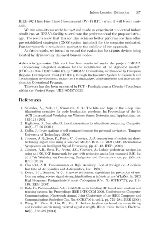

![SMACovid-19 – Autonomous Monitoring
System for Covid-19
Rui Fernandes(B)
and José Barbosa
MORE – Laboratório Colaborativo Montanhas de Investigação – Associação,
Bragança, Portugal
{rfernandes,jbarbosa}@morecolab.pt
Abstract. The SMACovid-19 project aims to develop an innovative
solution for users to monitor their health status, alerting health pro-
fessionals to potential deviations from the normal pattern of each user.
For that, data is collected, from wearable devices and through manual
input, to be processed by predictive and analytical algorithms, in order
to forecast their temporal evolution and identify possible deviations, pre-
dicting, for instance, the potential worsening of the clinical situation of
the patient.
Keywords: COVID-19 · FIWARE · Docker · Forecasting
1 Introduction
Wearable devices nowadays support many sensing capabilities that can be used
to collect data, related to the body of the person using the wearable. This allowed
for the development of health related solutions based on data collected from the
wearable devices for different purposes: for instance, in [1], the authors present
a system for automated rehabilitation, in [2] big data analysis is used to define
healthcare services. Nowadays, we are facing a pandemic scenario and this work
intends to use the characteristics of the wearable devices to develop an innovative
solution that can be used to diagnose possible infected COVID-19 patients, at
an early stage, by monitoring biological/physical parameters (through wearable
devices) and by conducting medical surveys that will allow an initial screening.
2 Docker and FIWARE
The system was developed using Docker compose, to containerize the architec-
ture modules, and FIWARE, to deal with the context information.
Docker is an open source platform that allows the containerization of appli-
cations and uses images and containers to do so. An image is a lightweight,
standalone, executable package of software that includes everything needed to
run an application: code, runtime, system tools, system libraries and settings [3].
c
Springer Nature Switzerland AG 2021
A. I. Pereira et al. (Eds.): OL2A 2021, CCIS 1488, pp. 309–316, 2021.
https://doi.org/10.1007/978-3-030-91885-9_22](https://image.slidesharecdn.com/optimizationlearningalgorithmsandapplications-231204021346-9e8015c0/85/Optimization-Learning-Algorithms-and-Applications-pdf-319-320.jpg)
![310 R. Fernandes and J. Barbosa
A container is a standardized unit of software, and includes the code as well as
the necessary dependencies for it to run efficiently, regardless of the computing
environment where is being run [3]. Images turn into containers at runtime. The
advantage that applications developed using this framework have is that they
will always run the same way, regardless of the used infrastructure to run them.
The system was developed using the FIWARE platform [4]. FIWARE defines
a set of standards for context data management and the Context Broker (CB)
is the key element of the platform, enabling the gathering and management of
context data: the current context state can be read and the data can be updated.
FIWARE uses the FIWARE NGSI RESTful API to support data transmis-
sion between components as well as context information update or consumption.
The usage of this open source RESTful API simplifies the process of adding extra
functionalities through the usage of extra FIWARE or third-party components.
As an example, FIWARE extra components, ready to use, cover areas such as
interfacing with the Internet of Things (IoT), robots and third-party systems;
context data/API management; processing, analysis and visualization of context
information. In this project, the version used was the NGSI-v2.
3 System Architecture
The system’s architecture is the one shown in Fig. 1, in which the used/
implemented modules communicate through the ports identified on the edges:
– Orion: FIWARE context broker;
– Cygnus: responsible for the data persistence in the MongoDB;
– Context Provider: performs data acquisition from the Fitbit API;
– Data analysis: processes the available data to generate forecasts;
– Fitbit API: data source for the wearable device.
In the system, data from the wearable device and from the mobile app
is posted into the CB. This data is automatically persisted in the MongoDB
through the cygnus module and is also used to trigger the data analysis module,
to execute a new forecast operation. Data persistence is implemented through
the creation of subscriptions in the CB that notify cygnus about data update.
There are already docker images ready to use for the standard modules,
such as, the MongoDB, the Orion context broker and the Cygnus persistence
module. The context provider and data analysis modules were developed and
containerized to generate the full system architecture.
3.1 Data Model
The NGSI-v2 API establishes rules for entity definition. Per those rules, an entity
has to have mandatory attributes, namely, the id and the type attributes. The
id is an unique uniform resource name (urn) created according with the format
“urn:ngsi-ld:entity-type:entity-id”.
In this work, the entity’s type is identified in each entity definition, as can
be seen in the data model presented in Fig. 2.](https://image.slidesharecdn.com/optimizationlearningalgorithmsandapplications-231204021346-9e8015c0/85/Optimization-Learning-Algorithms-and-Applications-pdf-320-320.jpg)
![SMACovid-19 – Autonomous Monitoring System for Covid-19 311
Fig. 1. Architecture devised to create the SMACovid-19 system.
Given the fact that each id has to be unique, the entity-id part of the urn
was created based on the version 4 of the universally unique identifier (uuid).
Using these rules, a person entity may be, for instance:
urn:ngsi-ld:Person:4bc3262c-e8bd-4b33-b1ed-431da932fa5
To define the data model, extra attributes were used, in each entity, to con-
vey the necessary information between modules. Thus, the Person entity has
attributes to specify the user characteristics and to associate the person with his
fitbit account. The Measurement entity represents the acquired data values and
its corresponding time of observation. This entity is used to specify information
regarding the temperature, oxygen saturation, blood pressure, heart rate and
daily number of diarrhea occurrences. The measurementType attribute is used
to indicate what type of variable is being used on that entity. To ensure max-
imum interoperability possible, the Fast Healthcare Interoperability Resources
(FHIR) specification of Health Level Seven International (HL7) [5] was used
to define terms whenever possible. This resulted in the following terms being
used: bodytemp for temperature, oxygensat for oxygen saturation, bp for blood
pressure, heartrate for heart rate and diarrhea (FHIR non-compliant) for daily
number of diarrhea occurrences.
The Questionnaire entity specifies data that has to be acquired through the
response of a questionnaire, by the user, through the mobile application. The
Organization entity identifies the medical facility that the person is associated
with. The Forecast entity provides the forecast mark value, calculated accord-](https://image.slidesharecdn.com/optimizationlearningalgorithmsandapplications-231204021346-9e8015c0/85/Optimization-Learning-Algorithms-and-Applications-pdf-321-320.jpg)
![312 R. Fernandes and J. Barbosa
Fig. 2. Data model
ing with the classification table defined by the Hospital Terra Quente (HTQ)
personnel, and the corresponding time of forecast calculation.
3.2 Data Acquisition
Data is acquired from two different sources: mobile application and Fitbit API.
The mobile application is responsible for manual data gathering, sending
this data to the CB through POST requests. For instance, data related to the
attributes of the Questionnaire entity is sent to the CB using this methodology.
Fitbit provides an API for data acquisition that, when new data is uploaded
to the Fitbit servers, sends notifications to a configured/verified subscriber end-
point. These notifications are similar to the one represented in Fig. 3. The
Fig. 3. Fitbit notification identifying new data availability [6].](https://image.slidesharecdn.com/optimizationlearningalgorithmsandapplications-231204021346-9e8015c0/85/Optimization-Learning-Algorithms-and-Applications-pdf-322-320.jpg)

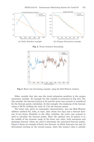
![316 R. Fernandes and J. Barbosa
available. The smoothing parameters α, β and γ fed into the Holt-Winters
method [7] were [0.5, 0.5, 0.5] respectively. The optimization yielded the values
[0.61136, 0.00189, 0.65050] with an associated MAE of 4.12.
Considering the forecast values, the minimum is 74.4983 and the maximum
is 84.2434, thus, the forecast points associated with this example, according with
Table 1, are 0 points.
5 Conclusions
In this work, we present a solution using mobile applications and wearable
devices for health data collection and analysis, with the purpose of generat-
ing health status forecasting, for patients that may, or may not, be infected with
the COVID-19 virus. To implement this solution, Docker containerization was
used together with elements from the FIWARE platform to create the system’s
architecture. A health context provider was implemented, to fetch data from the
wearable device, as well as a data analysis module to make the forecasts.
Three types of forecasts were devised, considering the variables characteris-
tics, namely, last observation, trend estimation and Holt-Winters methodology.
The obtained results so far are encouraging and future work can be done
in the optimization of the forecast methods and in the inclusion of more data
sources.
Acknowledgements. This work was been supported by SMACovid-19 – Autonomous
Monitoring System for Covid-19 (70078 – SMACovid-19).
References
1. Candelieri, A., Zhang, W., Messina, E., Archetti, F.: Automated rehabilitation exer-
cises assessment in wearable sensor data streams. In: 2018 IEEE International Con-
ference on Big Data (Big Data), pp. 5302–5304 (2018). https://doi.org/10.1109/
BigData.2018.8621958
2. Hahanov, V., Miz, V.: Big data driven healthcare services and wearables. In: the
Experience of Designing and Application of CAD Systems in Microelectronics, pp.
310–312 (2015). https://doi.org/10.1109/CADSM.2015.7230864
3. Docker. https://www.docker.com/resources/what-container. Accessed 5 May 2021
4. FIWARE. https://www.fiware.org/developers/. Accessed 5 May 2021
5. HL7 FHIR Standard. https://www.hl7.org/fhir/R4/. Accessed 5 May 2021
6. Fitbit Subscriptions Homepage. https://dev.fitbit.com/build/reference/web-api/
subscriptions/. Accessed 5 May 2021
7. Holt-Winters Definition. https://otexts.com/fpp2/holt-winters.html. Last accessed
5 May 2021. Accessed 5 May 2021](https://image.slidesharecdn.com/optimizationlearningalgorithmsandapplications-231204021346-9e8015c0/85/Optimization-Learning-Algorithms-and-Applications-pdf-326-320.jpg)

![Economic Burden of Personal Protective
Strategies for Dengue Disease:
an Optimal Control Approach
Artur M. C. Brito da Cruz1,3
and Helena Sofia Rodrigues2,3(B)
1
Escola Superior de Tecnologia de Setúbal, Instituto Politécnico de Setúbal,
Setúbal, Portugal
artur.cruz@estsetubal.ips.pt
2
Escola Superior de Ciências Empresariais, Instituto Politécnico de Viana
do Castelo, Valença, Portugal
sofiarodrigues@esce.ipvc.pt
3
CIDMA - Centro de Investigação e Desenvolvimento em Matemática e Aplicações,
Departamento de Matemática, Universidade de Aveiro, Aveiro, Portugal
Abstract. Dengue fever is a vector-borne disease that is widely spread.
It has a vast impact on the economy of countries, especially where the
disease is endemic. The associated costs with the disease comprise pre-
vention and treatment. This study focus on the impact of adopting
individual behaviors to reduce mosquito bites - avoiding the disease’s
transmission - and their associated costs. An epidemiological model is
presented with human and mosquito compartments, modeling the inter-
action of dengue disease. The model assumed some self-protection mea-
sures, namely the use of repellent in human skin, wear treated clothes
with repellent, and sleep with treated bed nets. The household costs for
these protections are taking into account to study their use. We con-
clude that personal protection could have an impact on the reduction of
the infected individuals and the outbreak duration. The costs associated
with the personal protection could represent a burden to the household
budget, and its purchase could influence the shape of the infected’s curve.
Keywords: Dengue · Economic burden · Personal protection ·
Household costs · Optimal control
1 Introduction
Dengue is a mosquito-borne disease dispersed almost all over the world. The
infection occurs when a female Aedes mosquito bites an infected person and
then bites another healthy individual to complete its feed [10].
According to World Health Organization (WHO) [27], each year, there are
about 50 million to 100 million cases of dengue fever and 500,000 cases of severe
Supported by FCT - Fundação para a Ciência e a Tecnologia.
c
Springer Nature Switzerland AG 2021
A. I. Pereira et al. (Eds.): OL2A 2021, CCIS 1488, pp. 319–335, 2021.
https://doi.org/10.1007/978-3-030-91885-9_23](https://image.slidesharecdn.com/optimizationlearningalgorithmsandapplications-231204021346-9e8015c0/85/Optimization-Learning-Algorithms-and-Applications-pdf-328-320.jpg)
![320 A. M. C. Brito da Cruz and H. S. Rodrigues
dengue, resulting in hundreds of thousands of hospitalizations and over 20,000
deaths, mostly among children and young adults.
Several factors contribute to this public health problem, such as uncontrolled
urbanization and increasing population growth. Problems like the increased use
of non-biodegradable packaging coupled with nonexistent or ineffective trash
collection services, or the growing up number of travel by airplane, allowing
the constant exchange of dengue viruses between countries, reflect such factors.
Besides, the financial and human resources are limited, leading to programs that
emphasize emergency control in response to epidemics rather than on integrated
vector management related to prevention [27].
These days, dengue is one of the most important vector-borne diseases and,
globally, has heavy repercussions in morbidity and economic impact [1,28].
1.1 Dengue Economic Burden
Stanaway et al. [25] estimated dengue mortality, incidence, and burden for the
Global Burden of Disease Study. In 2013, there were almost 60 million symp-
tomatic dengue infections per year, resulting in about 10 000 deaths; besides, the
number of symptomatic dengue infections more than doubled every ten years.
Moreover, Shepard et al. [23] estimated a total annual global cost of dengue
illness of US$8.9 billion, with a distribution of dengue cases of 18% admitted to
hospital, 48% ambulatory, and 34% non-medical.
Dengue cases have twofold costs, namely prevention and treatment. The
increasing of dengue cases leads to the rise of health expenditures, such as outpa-
tient, hospitalization, and drug administration called direct costs. At the same
time, there are indirect costs for the economic operation, such as loss of pro-
ductivity, a decrease in tourism, a reduction in foreign investment flows [14].
Most of the countries only bet on prevention programs to control the outbreaks.
They focus on the surveillance program, with ovitraps or advertising campaigns
regarding decrease the breeding sites of the mosquito.
1.2 Personal Protective Measures (PPM)
Another perspective on dengue prevention is related to household prevention,
where the individual has a central role in self-protection. PPM could be physical
(e.g., bed nets or clothing) or chemical barriers (e.g., skin repellents).
Mosquito nets are helpful in temporary camps or in houses near biting insect
breeding areas. Care is needed not to leave exposed parts of the body in contact
with the net, as mosquitoes bite through the net. However, insecticide-treated
mosquito nets have limited utility in dengue control programs, since the vector
species bite during the day, but treated nets can be effectively utilized to protect
infants and night workers who sleep by day [18].
For particular risk areas or occupations, the protective clothing should be
impregnated with allowed insecticides and used during biting insect risk periods.](https://image.slidesharecdn.com/optimizationlearningalgorithmsandapplications-231204021346-9e8015c0/85/Optimization-Learning-Algorithms-and-Applications-pdf-329-320.jpg)
![Economic Burden of Personal Protective Strategies for Dengue Disease 321
Repellents with the chemical diethyl-toluamide (DEET) give good protec-
tion. Nevertheless, repellents should act as a supplementary to protective cloth-
ing.
The population also has personal expenses to prevent mosquito bites. There
are on the market cans of repellent to apply on the body, clothing already impreg-
nated with insect repellent, and mosquito bed nets to protect individuals when
they are sleeping. All of these items have costs and are considered the household
cost for dengue.
The number of research papers studying the dengue impact dengue on the
country’s economy is considerable [9,11,13,23,24,26]. However, there is a lack of
research related to household expenditures, namely what each individual could
spend to protect themselves and their family from the mosquito. There is some
work available about insecticide bed nets [19] or house spraying operations [8],
but there is a lack of studies using these three PPM in the scientific literature.
Each person has to make decisions related to spending money for its protec-
tion or risking catching the disease.
This cost assessment can provide an insight to policy-makers about the eco-
nomic impact of dengue infection to guide and prioritize control strategies.
Reducing the price or attribute subsidies for some personal protection items
could lead to an increase in the consumption of these items, and therefore, to
prevent mosquito bites and the disease.
This paper studies the influence of the price of personal protection to prevent
dengue disease from the individual perspective. Section 2 introduces the optimal
control problem, the parameter, and the variables that composed the epidemio-
logical model. Section 3 analyzes the numerical results, and Sect. 4 presents the
conclusions of the work.
2 The Epidemiological Model
2.1 Dengue Epidemiological Model
This research is based on the model proposed by Rodrigues et al. [21], where
it is studied the human and mosquito population through a mutually exclu-
sive compartmental model. The human population is divided in the classic SIR-
type epidemiological framework (Susceptible - Infected - Recovered), while the
mosquito population only has two components SI (Susceptible - Infected). Some
assumptions are assumed: both (humans and mosquitoes) are born susceptibles;
there is homogeneity between host and vectors; the human population is con-
stant (N = S + I + R), disregarding migrations processes; and seasonality was
not considered, which could influence the mosquito population.
The epidemic model for dengue transmission is given by the following sys-
tems of ordinary differential equations for human and mosquito populations,
respectively.](https://image.slidesharecdn.com/optimizationlearningalgorithmsandapplications-231204021346-9e8015c0/85/Optimization-Learning-Algorithms-and-Applications-pdf-330-320.jpg)
![322 A. M. C. Brito da Cruz and H. S. Rodrigues
⎧
⎪
⎪
⎪
⎪
⎪
⎨
⎪
⎪
⎪
⎪
⎪
⎩
dS(t)
dt
= μhNh −
Bβmh
Im(t)
Nh
+ μh
S(t)
dI(t)
dt
= Bβmh
Im(t)
Nh
S(t) − (ηh + μh) I(t)
dR(t)
dt
= ηhI(t) − μhR(t)
(1)
⎧
⎪
⎪
⎨
⎪
⎪
⎩
dSm(t)
dt
= μmNm −
BβhmI(t)
Nh
+ μm
Sm(t)
dIm(t)
dt
= Bβhm
I(t)
Nh
Sm(t) − μmIm(t)
(2)
As expected, these systems depict the interactions of the disease between
humans to mosquitoes and vice-versa. Parameters of the model are presented in
Table 1.
Table 1. Parameters of the epidemiological model
Parameter Description Range Used values Source
Nh Human population 112000 [12]
1
μh
Average lifespan of humans
(in days)
79 × 365 [12]
B Average number of bites
on an unprotected person
(per day)
1
3
[20,21]
βmh Transmission probability
from Im (per bite)
[0.25, 0.33] 0.25 [6]
1
ηh
Average infection period on
humans (per day)
[4, 15] 7 [4]
1
μm
Average lifespan of adult
mosquitoes (in days)
[8, 45] 15 [7,10,16]
Nm Mosquito population 6 × Nh [22]
βhm Transmission probability
from Ih (per bite)
[0.25, 0.33] 0.25 [6]
This model does not incorporate any PPM. Therefore we need to add another
compartment to the human population: the Protected (P) compartment. It com-
prises humans that are using personal protection, and therefore they cannot be
bitten by mosquitoes and getting infected.
It is introduced a control variable u(·) in (1), which represents the effort of
taking PPM. Additionally, a new parameter is required, ρ, depicting the pro-
tection duration per day. Depending on the PPM used, this value is adequate](https://image.slidesharecdn.com/optimizationlearningalgorithmsandapplications-231204021346-9e8015c0/85/Optimization-Learning-Algorithms-and-Applications-pdf-331-320.jpg)
![Economic Burden of Personal Protective Strategies for Dengue Disease 323
for the individual protection capacity [5]. To reduce computational errors, it
was normalized the differential equations, meaning that the proportions of each
compartment of individuals in the population were considered, namely
s =
S
Nh
, p =
P
Nh
, i =
I
Nh
, r =
R
Nh
and
sm =
Sm
Nm
, im =
Im
Nm
The model with control is defined by:
⎧
⎪
⎪
⎪
⎪
⎪
⎪
⎪
⎪
⎨
⎪
⎪
⎪
⎪
⎪
⎪
⎪
⎪
⎩
ds(t)
dt
= μh − (6Bβmhim(t) + u(t) + μh) s(t) + (1 − ρ)p(t)
dp(t)
dt
= u(t)s(t) − ((1 − ρ) + μh) p(t)
di(t)
dt
= 6Bβmhim(t)s(t) − (ηh + μh) i(t)
dr(t)
dt
= ηhi(t) − μhr(t)
(3)
and
⎧
⎪
⎨
⎪
⎩
dsm(t)
dt
= μm − (Bβhmi(t) + μm) sm(t)
dim(t)
dt
= Bβhmi(t)sm(t) − μmim(t)
(4)
This set of equations is subject to the initial equations [21]:
s(0) =
11191
Nh
, p(0) = 0, i(0) =
9
Nh
, r(0) = 0, sm(0) =
66200
Nm
, im(0) =
1000
Nm
.
(5)
The mathematical model is represented by the epidemiological scheme in
Fig. 1.
Due to the impossibility of educating everyone to use PPM, namely because
of budget constraints, time restrictions, or even the low individual willingness
to using PPM, it is considered that the control u(·) is bounded between 0 and
umax = 0.7.
2.2 Optimal Control Problem
In this section, an optimal control problem is proposed that portrays the costs
associated with PPM and the restrictions of the epidemy.
The objective functional is given by
J(u(·)) = R(T) +
T
0
γu2
(t)dt (6)](https://image.slidesharecdn.com/optimizationlearningalgorithmsandapplications-231204021346-9e8015c0/85/Optimization-Learning-Algorithms-and-Applications-pdf-332-320.jpg)
![324 A. M. C. Brito da Cruz and H. S. Rodrigues
Fig. 1. Flow diagram of Dengue model with personal protection strategies
where γ is a constant that represents the cost of taking personal prevention
measures per day and person. At the same time, it is relevant that this functional
also has a payoff term: the number of humans recovered by disease at the final
time, R(T). It is expected that the outbreak dies out, and therefore, the total
of recover individuals gives the cumulative number of persons infected by the
disease. We want to minimize the total number of infected persons, and therefore
recovered persons at the final time and the expenses associated with buying
protective measures.
Along time, we want to find the optimal value u∗
of the control u, such that
the associated state trajectories S∗
, P∗
, I∗
, R∗
, S∗
m, I∗
m are solutions of the Eqs.
(3) and (4) with the following initial conditions:
s(0) ⩾ 0, p(0) ⩾ 0, i(0) ⩾ 0, r(0) ⩾ 0, sm(0) ⩾ 0, im(0) ⩾ 0. (7)
The set of admissible controls is
Ω = {u(·) ∈ L∞
[0, T] : 0 ⩽ u(·) umax, ∀t ∈ [0, T]}.
The optimal control consists of finding (s∗
(·), p∗
(·), i∗
(·), r∗
(·), s∗
m(·), i∗
m(·))
associated with an admissible control u∗
(·) ∈ Ω on the time interval [0, T] that
minimizes the objective functional.
Note that the cost function is L2
and the integrand function is convex with
respect to the function u. Furthermore, the control systems are Lipschitz with
respect to the state variables and, therefore, exists an optimal control [3].
The Hamiltonian function is
H = H (s(t), p(t), i(t), r(t), sm(t), im(t), Λ, u(t)) = γu2
(t)
+ λ1 (μh − (6Bβmhim(t) + u(t) + μh) s(t) + (1 − ρ)p(t))
+ λ2 (u(t)s(t) − ((1 − ρ) + μh) p(t))
+ λ3 (6Bβmhim(t)s(t) − (ηh + μh) i(t))
+ λ4 (ηhi(t) − μhr(t))
+ λ5 (μm − (Bβhmi(t) + μm) sm(t))
+ λ6 (Bβhmi(t)sm(t) − μmim(t))](https://image.slidesharecdn.com/optimizationlearningalgorithmsandapplications-231204021346-9e8015c0/85/Optimization-Learning-Algorithms-and-Applications-pdf-333-320.jpg)
![Economic Burden of Personal Protective Strategies for Dengue Disease 325
Pontryagin’s Maximum Principle [17] states that if u∗
(·) is optimal control
for the equations (3)–(6) with fixed final time, then there exists a nontrivial
absolutely continuous mapping, the adjoint vector:
Λ : [0, T] → R6
, Λ(t) = (λ1(t), λ2(t), λ3(t), λ4(t), λ5(t), λ6(t))
such that
s
=
∂H
∂λ1
, p
=
∂H
∂λ2
, i
=
∂H
∂λ3
, r
=
∂H
∂λ4
, s
m =
∂H
∂λ5
and i
m =
∂H
∂λ6
,
and where the optimality condition
H (s∗
(t), p∗
(t), i∗
(t), r∗
(t), s∗
m(t), i∗
m(t), Λ(t), u∗
(t))
= min
0⩽uumax
H (s∗
(t), p∗
(t), i∗
(t), r∗
(t), s∗
m(t), i∗
m(t), Λ(t), u(t))
and the transversality conditions
λi(T) = 0, i = 1, 2, 3, 5, 6 and λ4(T) = 1 (8)
hold almost everywhere in [0, T] .
The following theorem follows directly from applying the Pontryagin’s max-
imum principle to the optimal control problem.
Theorem 1. The optimal control problem with fixed final time T defined by the
Eqs. (3)–(6) has a unique solution (s∗
(t), p∗
(t), i∗
(t), r∗
(t), s∗
m(t), i∗
m(t)) associ-
ated with the optimal control u∗
(· · · ) on [0, T] given by
u∗
(t) = max 0, min
(λ1(t) − λ2(t)) s∗
(t)
2γ
, umax (9)
with the adjoint function satisfying
⎧
⎪
⎪
⎪
⎪
⎪
⎪
⎪
⎪
⎨
⎪
⎪
⎪
⎪
⎪
⎪
⎪
⎪
⎩
λ
1(t) = λ1 (6Bβmhi∗
m(t) + u∗
(t) + μh) − λ2u∗
(t) − λ36Bβmhi∗
m(t)
λ
2(t) = −λ1(1 − ρ) + λ2 ((1 − ρ) + μh)
λ
3(t) = λ3 (ηh + μh) − λ4ηh + (λ5 − λ6) Bβhms∗
m(t)
λ
4(t) = λ4μh
λ
5(t) = λ5 (Bβhmi∗
(t) + μm) − λ6Bβhmi∗
(t)
λ
6(t) = (λ1 − λ3) 6Bβmhs∗
(t) + λ6μm
(10)
3 Numerical Results
This section presents the results of the numerical implementation of control
strategies for PPM for dengue disease.](https://image.slidesharecdn.com/optimizationlearningalgorithmsandapplications-231204021346-9e8015c0/85/Optimization-Learning-Algorithms-and-Applications-pdf-334-320.jpg)
![326 A. M. C. Brito da Cruz and H. S. Rodrigues
For the problem resolution, the time frame considered was one year, and the
parameters used are available on Table 1.
To obtain the computational results, Theorem 1 was implemented numeri-
cally on MATLAB version R2017b and the extremal found, u∗
, was evaluated
using a forward-backward fourth-order Runge-Kutta method with a variable
time step for efficient computation (see [15] for more details). For the differen-
tial equations related to the state variables, (3)–(4) it was performed a forward
method using the initial conditions (5). For the differential equations related
to adjoint variables, it was applied a backward system using the transversality
conditions (8).
Figure 2 shows the evolution of the human state variables during the whole
year, without any control. This analysis is a meaningful kickoff point to make a
fair comparison with the application of the PPM. It should also be mentioned
that this model does not take into account deaths by dengue, because in the
considered region of the study [21], fortunately, nobody died, and there were no
cases of hemorrhagic fever.
Fig. 2. Evolution of human state variables when human population did not take any
protective measures
For this research, three protective measures were considered: insect repellent,
bed nets, and clothes impregnated with insect repellent. It was obtained the
average price of each product on the market as well as how long each product
stays active.
The following simulations are divided into two subsections: the first one,
using only one PPM, and the second one, where several PPM are combined.
Each PPM has two factors associated: cost and durability. In our model, the
parameter γ is the cost that each individual spends to protect themself during](https://image.slidesharecdn.com/optimizationlearningalgorithmsandapplications-231204021346-9e8015c0/85/Optimization-Learning-Algorithms-and-Applications-pdf-335-320.jpg)

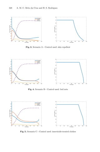
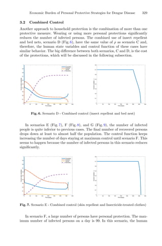
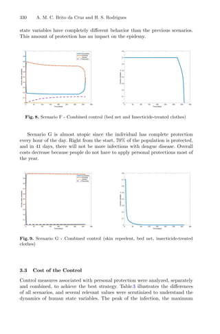

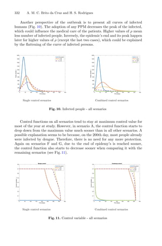
![Economic Burden of Personal Protective Strategies for Dengue Disease 333
Protective measures have varied prices, and the duration that each one lasts is
different. Scenarios F and G seem to prove that the use of very efficient protection
from the start of the outbreak, ends it sooner. Furthermore, and possibly not
expected, each person in these scenarios does not spend as much money as in
other cases. For instance, scenario F appears to be a much better solution than
scenario E, not only for personal cost but also to fight the disease.
4 Conclusions
Effective dengue prevention requires a coordinated and sustainable approach.
This way, it is possible to address environmental, behavioral, and social con-
texts of disease transmission. Determining household expenditure related to bite
prevention is a crucial purpose for acting in advance of an outbreak. With an
efficient cost analysis, each individual could make a trade-off decision between
the available resources.
This work is the follow up work that the authors started in [2]. In here, the
research tried to answer the following question: what is the best strategy to fight
dengue disease and, at the same time, spending less money?
The results corroborated that if one person is more protected, then the disease
spreads less. Long protection flattens the infected human curve, which is a good
perspective from the medical point of view. Hence, the medical staff could have
more time to prepare the outbreak response, and the Heath Authorities could
acquire more supplies to treat the patients.
However, it was found that does not mean that the person should spend
more. As an example, the protection used with skin repellent and bed net has
the same impact on the number of infected individuals when compared with the
insecticide-treated clothes, but it is much cheaper.
These results also reflect the importance of using personal protective mea-
sures for most part of the day. Half or even more of the population will not be
infected if at least 16 h a day a person stays protected.
As future work, it will be interesting to study the economic impact of strate-
gies related to prevention - including self-protect measures - and treatment -
that could including costs with drug administration, hospitalization, or even sick
days losses, focusing only on the individual perspective. Another perspective to
be implemented is to analyze the economic evaluation of prevention. The adop-
tion of some prevention activities, from the individual point of view, could have
a profound impact on the government budget allocated to the disease’s treat-
ment. Thus could be critical to investigate the financial support of preventive
measures.
Acknowledgement. This work is supported by The Center for Research and Develop-
ment in Mathematics and Applications (CIDMA) through the Portuguese Foundation
for Science and Technology (FCT - Fundação para a Ciência e a Tecnologia), references
UIDB/04106/2020 and UIDP/04106/2020.](https://image.slidesharecdn.com/optimizationlearningalgorithmsandapplications-231204021346-9e8015c0/85/Optimization-Learning-Algorithms-and-Applications-pdf-342-320.jpg)


![ERP Business Speed – A Measuring Framework
Zornitsa Yordanova(B)
University of National and World Economy, 8mi dekemvri, Sofia, Bulgaria
zornitsayordanova@unwe.bg
Abstract. A major business problem nowadays is how adequate and appropriate
the ERP system used is for growing business needs, the ever-changing complexity
of the business environment, the growing global scale competition, and as a result
- the growing speed of business. The purpose of this research is to make the bench-
mark for an ERP system business speed (performance from a business operations
point of view), i.e. how fast the business operations executed are with the used
ERP. A literature analysis is conducted for framing and defining the concept of
ERP business speed as an important and crucial factor for business success. Then a
measurement framework for testing ERP systems in terms of business operations
and ERP business performance is proposed and tested. Metrics for measuring ERP
business speed are defined by conducting focused interviews with experts in ERP
implementation and maintenance. The measurement framework has been empir-
ically tested in 6 business organizations, first to validate the selected KPIs and
second to formulate some average business speed indications of the KPIs as part
of the business speed of ERP. The research contributes by providing a framework
measurement tool for testing business speed of ERP systems. The study can also
serve as a benchmark in further measuring of ERP business speed. From theory
perspective, this study provides a definition and an explanation of the term ERP
business speed for the first time in the literature.
Keywords: ERP · Enterprise information systems · Enterprise software ·
Business speed · MIS · Measurement tool
1 Introduction
Enterprise resource planning (ERP) is an integrated management approach for organi-
zations that aims at encompassing all enterprise activities into a system process moving
together [1]. Nowadays these systems are usually integrated into an information system
because of the large scope of business, huge number of transactions, complex inter-
nal processes, competiveness and optimization efforts for achieving higher margin [2].
Enterprise resource planning systems are integrated software packages, including all
necessary ingredients that would support the smooth work flow and process with a
common database [3]. They are used for integration and automation of the processes,
performance improvements, and cost reduction of all enterprise activities [4]. They are
considered as powerful tool for enterprise management and information and data man-
agement for reducing human error, speed the flow of information, and improve overall
© Springer Nature Switzerland AG 2021
A. I. Pereira et al. (Eds.): OL2A 2021, CCIS 1488, pp. 336–344, 2021.
https://doi.org/10.1007/978-3-030-91885-9_24](https://image.slidesharecdn.com/optimizationlearningalgorithmsandapplications-231204021346-9e8015c0/85/Optimization-Learning-Algorithms-and-Applications-pdf-345-320.jpg)
![ERP Business Speed – A Measuring Framework 337
decision making throughout the organization [5]. Over the last two decades, ERP sys-
tems have become one of the most significant and expensive implementations in the
information technology business [6]. Because of their impotence for businesses and
wide-spreading amongst enterprises, any kind of new technology or business issue has
been shortly incorporated within ERPs [4] and they have become an integral part of
enterprises addressing changing environment, the increasing market requirements and
increased data needs of enterprises. Yet, ERP requires large amount of investment, time,
resources and efforts and a potential failure is a risky factor [7] that many companies
consider as frightening and still feasible [8].
However, at the beginning of the third decade of 21st century, the question for the
benefit from implementing ERP system is not relevant anymore. Now the question is
not how fast, easy and effective to implement an ERP, but rather it is how the already
implemented ERP serve the organizations’ needs and how fast it answers to their business
speed [9]. The research question of this study is what is ERP business speed and how it
could be measured.
2 Theoretical Background
2.1 ERP Systems and Their Significance for Businesses
ERP systems have been designed to address the fragmentation and decomposition of
information transaction by transaction across an enterprise’s business, and also to inte-
grate with intra- and inter- enterprise information [10]. They are usually organized
in complex software packages which integrate data, information and business process
across functional areas of business [11]. ERP systems are customer-tailored and usually
customized into a unique system that fulfil individual and specific needs [12]. ERP sys-
tems aims at covering the full range of functionality needed by organizations and this
is considered as their main benefit [13]. Implementation of an ERP system across an
organization takes time, money and a lot of efforts, including internal resources [14].
That is why organizations have been trying hard to find out and come up with factors that
can help them to succeed in their implementation of ERP systems [15]. There are a lot of
researches examining ERP implementation failure factors [16] and project management
approaches [17] so to optimize these implementations and ERP utilization. Nowadays,
ERP researches are focused more on ERP transformation according to the changes [18].
ERP are closely tighten with business and [19] defines ERP is an institutionalized fac-
tor and component of enterprise infrastructure and development. Davenport [20] stated
even 20 years ago that the business world embraced ERP and that might be the most
important development in the corporate use of information technology came from the
90s. But the science literature provides many proves that still it is important in 2020
[21]. ERP systems are crucial for business from operational point of view and functional
capabilities [22] but also are considered as critically needed for top management who
reckon them as an important tool for both strategic and operative purposes [23].
For some organizations, ERP is a mandatory factor for operating [24]. ERP systems
benefit organizations by improving the quality of service and increasing efficiency [25].
ERP systems have transformed the functioning of firms with regard to higher efficiency
and accuracy in their operations [7]. Poston and Grabski [21] examined enterprises](https://image.slidesharecdn.com/optimizationlearningalgorithmsandapplications-231204021346-9e8015c0/85/Optimization-Learning-Algorithms-and-Applications-pdf-346-320.jpg)
![338 Z. Yordanova
before and after adoption and found out a significant cost reduction. Hunton et al. [22]
did an experiment with financial analysts, researching whether investors consider ERP
implementation enhances firm value. The results showed positive effects from such
implementations even though that positive assumption was not measurable. According
Hedman and Kalling [23] main benefit from ERP and enterprise information systems at
all as well as factors that generate profit are the activation of the resource and activities,
and the quality and cost of the offering in the light of competition.
Generally, from business point of view, computing and ERP provides great additional
business value to business [26] and most of the analysed studies give arguments about
this cliché statement. Therefore, the focus of the current research falls on a relatively
new aspect of business and ERP that extend these systems’ significance from business
point of view. This new aspect is business speed and ERP business speed in particular.
2.2 Business Speed Requirements
Esteves and Pastor [25] researched ERP lifecycle and distinguish 6 phases of their usage
and utilization: decision, acquisition, implementation, use and maintenance, evolution,
and retirement phase. Nowadays, most of the implemented ERP systems have already
reached to the retirement phase because of new technologies [26] or because the currently
used ERP system or processes have become inadequate to the business’ needs [27]. As
a result, the ERP implementation is not a factor, a risk, a question or a doubt anymore.
After moving through all of these phases, acquisitions, deployment, use, maintenance
and evolution, the business’s interest in these already proven information systems is
directed at their business speed addressing real business goals. ERP business speed is
a novel term, first presented in this research. It should not be mixed up with economic
speed or business speed in general not with technology or technology adoption speed.
ERP business speed will be discussed in the next sections of the study. It is based on the
concept of business speed as it is increasingly important for businesses.
Business speed has already been met in the literature, but its meaning was never
fully defined and it was used as word combination rather than as a term [28]. The
word combination was used in different context. Bill Gates [29] used business speed
in his first book with meaning of the speed of business thought, how business, leaders
and technology should act together and where business goes to. His usage of business
speed is related to business direction and increasing the business cycles and changes in
general. Pulendran, Speed and Widing [30] use the word combination to explain business
performance. Meyer and Davis [31] used business speed from the prospective of speed of
change in the connected economy. For many researchers, business speed is modelling a
business approach that boost business [32]. For Gregory and Rawling [33] business speed
is related to time-based strategy, time compression and business performance. Miller [34]
was amongst the first ones linking business speed to information systems and addressed
business speed as acceleration of business via implementing SAP. Kaufmann and Wei
[35] examine business speed as commerce speed. Some authors have tried to connect
business speed with the startup ecosystem and some methods for startup management
as Lean startup method [36]. However, the linkage between ERP and business speed has
not yet been researched.](https://image.slidesharecdn.com/optimizationlearningalgorithmsandapplications-231204021346-9e8015c0/85/Optimization-Learning-Algorithms-and-Applications-pdf-347-320.jpg)

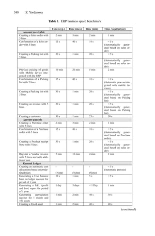
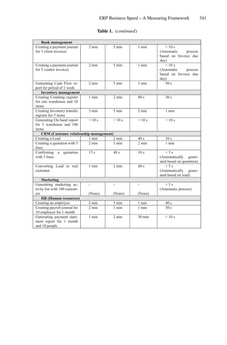
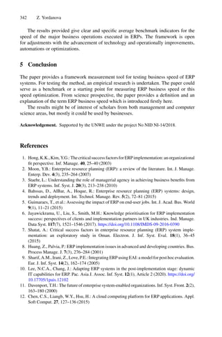


![346 J. P. Coelho et al.
input-to-output voltage ratio depends on the duty cycle imposed to those switch-
ing devices by a controller. This controller operates in closed-loop by sampling
the output voltage and comparing it with the desired output voltage value and
the difference between those two values will be used to establish the switching
duty-cycle. The block diagram presented in Fig. 1 illustrate this methodology.
Fig. 1. Typical feedback control architecture used in DC/DC converters.
Often, in practice, a current loop is also added in order to enable current-
mode control. This additional control layer enables overcurrent protection and
reduces the sensitivity of the voltage controller to the capacitor’s ESR. However,
in this paper, only the voltage-mode control is taken into consideration. Voltage-
mode control resort to feedback to keep constant the output voltage despite
unwanted disturbances. The loop compensation network associated to the error
amplifier can be of type I, II or III. Type I is a simple pole at the origin and type
II expand it by including a zero and a high-frequency pole which can leading to
a phase increase of 90o
. Finally, type III adds two poles and two zeros to the
pole at zero which promotes an increase in phase margin.
Those loop compensation circuits are tuned to perform well in a given nom-
inal system operating point. However, if the system deviates from this point,
the controller performance can become very poor. For example, when the power
supply shift between continuous to discontinuous conduction mode. Hence, adap-
tiveness and learning ability must be included in the controller in order for it
to be able to perform well in a large dynamic range and under the presence of
system changes.
This work proposes an alternative controller structure applied to regulate the
operation of a DC to DC buck converter. In particular, it will rely on the use
of control paradigm inspired on the brain emotional learning ability (BELBIC)
to promote adaption to operating point changes. Conceptually, this controller is
inspired by the brain’s limbic system and, when compared to the typical buck
converter controller, its most notorious property is the ability to keep learning
while in operation. The use of BELBIC was already applied within the power
electronics context. In [1], a brain emotional learning approach was employed in
the context of a maximum power-point tracking algorithm applied to solar energy
conversion. Additionally, in [2], a BELBIC controller was applied to control a](https://image.slidesharecdn.com/optimizationlearningalgorithmsandapplications-231204021346-9e8015c0/85/Optimization-Learning-Algorithms-and-Applications-pdf-355-320.jpg)
![348 J. P. Coelho et al.
Assuming small magnitudes of the disturbances, compared to the DC quies-
cent values, it is possible to obtain the following differential equations [3]:
L
d
dt
îL(t) = Dv̂g(t) + ˆ
d(t)Vg − v̂o(t) (1a)
C
d
dt
v̂o(t) = îL(t) −
v̂o(t)
Ro
(1b)
îg = DîL(t) + iL(t) ˆ
d(t) (1c)
where the hat symbol over the variables denotes a small disturbance around the
variable’s operating point and D is the PWM duty cycle whose value is within
the interval [0, 1].
After applying the Laplace transform to the previous set of differential equa-
tions, the transfer function between the output and the command signal, denoted
by Gvod(s), is:
Gvod(s) =
v̂o(s)
ˆ
d(s)
=
RoVg
LCRos2 + Ls + Ro
(2)
and from input to output voltage, Gvovg
(s), defined as:
Gvovg
(s) =
v̂o(s)
v̂g(s)
=
RoD
LCRos2 + Ls + Ro
(3)
Without input voltage disturbances or load changes, the converter is able to
operate in open-loop. However, the output value can fluctuates in the presence
of load changes of other disturbances as input voltage drops/rises or shifts in
the components nominal values due to several factors such as aging. Thus, a
closed-loop controller must be added in order to regulate the switched converter
voltage output.
Typically, type I, II or III loop compensator structures are chosen to carry out
this task and can be designed using the previously defined transfer functions.
However, it is worth to notice that those transfer functions are only approxi-
mations and assumes small disturbances around a given operating point. For
this reason, the behaviour of the switching converter can be very different out-
side the defined zone. Specially, if due to small loads, the converter settles to
work in discontinuous conduction mode. Fixed poles-zeros controller are unable
to achieve good performance in the presence of severe changes in the system
dynamic behaviour. Other approach is to enable the controller to learn and use
this knowledge to self adjust its behaviour in order to increase the overall per-
formance within a broader range of operating points. In this work, this feature
will be attained by resorting to a soft-computing paradigm known by BELBIC
and briefly described in the following section.
3 The BELBIC Controller
From an engineering point-of-view, analysis of the solutions produced by nature
to overcome the animal species adaption problems, have led to an increasing](https://image.slidesharecdn.com/optimizationlearningalgorithmsandapplications-231204021346-9e8015c0/85/Optimization-Learning-Algorithms-and-Applications-pdf-357-320.jpg)
![BELBIC Based Step-Down Controller Design Using PSO 349
tendency to introduce bio-morphism and bio-mimicry in many different compu-
tational tools [4]. For example, biological inspiration can be tracked in appli-
cations such as machine cooperation, speech recognition, text recognition and
self-assembly nanotechnology just to name a few. All those examples have, in
fact that all rely on algorithms which have the capability of adaptation and
learning. Indeed, and in the biological realm, learning is one of the most impor-
tant factors for the endurance of all species. Learning allow the organisms to
adjust themselves to cope with changes in environmental and operating condi-
tions. This robustness is a desired characteristic in engineering applications since
the operating conditions of a product are never static. For this reason, simplified
approaches of some natural learning processes have been adapted to serve in
many engineering problems.
In the particular case of humans, learning takes place within generations and
across generations at many different levels. We are not talking only about intel-
lectual learning but also about the learning that is passed through our genome.
All this information shapes the actions of an individual when subject to a set
of environmental stimuli. At the mental level, reasoning is not the only driving
action when decision-making is concerned. Human reactions strongly depend
also on emotions and they play an important role in our everyday life and have
been a valuable asset in our survival and adaptation.
Is generally considered true that emotions were included during the evolu-
tionary stage as a way to reduce the human’s reaction time. That is, rather than
using the intellect to process information and generate actions, which would
take time, the reaction by emotion would be much faster. Emotions can then be
viewed as an automatic behaviour that seeks to improve survival by increasing
the ability to react fast in the presence of threats. It seems that the overall set
of possible emotions are predefined in our genome. However, they can then be
utterly modified based on the person’s individual experience.
Psychology and neural sciences circumscribe emotional activity to a set of
distinct brain regions gathered in what is known as the limbic region. Besides
emotions, the limbic system manages a distinct number of other functions such
as behaviour, motivation and has an important role in memory formation tasks.
At the present, it is still not consensual in the scientific community about which
brain areas should be included in the limbic system. However, it is commonly
accepted that the thalamus, hypothalamus, hippocampus and amygdala are the
main brain structures in the limbic system. Details regarding the role played by
each one of those cortical areas are outside the scope of this work. Instead, the
objective is to convert the limbic system behaviour, from a high-level abstraction
angle, and frame it in the context of computational intelligence. The first step
toward this approach was carried out by [5] by presenting a first mathematical
approach to describe the behaviour of the brain’s emotional learning (BEL) pro-
cess. The idea of applying this learning algorithm in the automatic control area
was provided, a couple of years later, by [6]. The junction of BEL with control
systems design has led to the concept known as “brain emotional learning-based](https://image.slidesharecdn.com/optimizationlearningalgorithmsandapplications-231204021346-9e8015c0/85/Optimization-Learning-Algorithms-and-Applications-pdf-358-320.jpg)
![350 J. P. Coelho et al.
intelligent control” (BELBIC). Further details regarding the operational details
of this control method can be found at [7–10].
The major pitfalls of BELBIC regards the choice of both emotional and
sensory signals in order to maximize the control system performance. Besides
that, several tuning parameters, such as the learning rate of the amygdala and
orbitofrontal processing units, must be found to achieve an acceptable controller
behaviour. The values for such parameters are commonly found by trial-and-
error which can be cumbersome and lead to suboptimal solutions. For those
reasons, other tuning methods have been presented [11–13] among them the use
of evolutionary based algorithms [14–18].
Due to its ability to provide good results for non-convex problems, evolu-
tionary algorithms have been employed in a myriad of different applications. For
this reason, in this work the BELBIC controller will be tuned by resorting to
the particle swarm optimization algorithm. A short overview on this method is
provided in the following section and further details on the methodology will be
described in Sect. 5.
4 The PSO Algorithm
The particle swarm optimisation (PSO) algorithm is fundamentally based
on the social behaviour of animals that moves in herds or flocks [19]. In
this algorithm, a set of particles, representing potential problem solutions
moves through the search space according to a given position vector xi(t) =
{xi1(t), xi2(t), · · · , xin(t)} and velocity vi(t) = {vi1(t), vi2(t), · · · , vin(t)} where
t denotes the current evolutionary iteration and n the number of particles.
The PSO dynamics is governed by individual and social knowledge. That is, a
given particle movement is due to it’s own experience and from social information
sharing. In [19] this concept was mathematically expressed by the following set
of equations:
coid(t) = (pid (t) − xid (t)) (4a)
soid(t) = (pgd (t) − xid (t)) (4b)
where coid(t) is the cognition-only value associated to the dth
dimension of the
ith
particle and soid(t) is the social-only component of the same individual.
The momentum and position of a given particle are computed by:
vid (t + 1) = vid (t) + ϕ1.coid(t) + ϕ2.soid(t) (5a)
xid (t + 1) = xid (t) + vid (t + 1) (5b)
where pid(t) concerns the best previous position of particle i in the current itera-
tion t and pgd(t) denotes the global best particle within a given neighbourhood.
The coefficient ϕ1 is the cognitive constant and ϕ2 is the social coefficient. Gen-
erally they are assumed to be uniformly distributed random numbers between
zero and two.](https://image.slidesharecdn.com/optimizationlearningalgorithmsandapplications-231204021346-9e8015c0/85/Optimization-Learning-Algorithms-and-Applications-pdf-359-320.jpg)
![BELBIC Based Step-Down Controller Design Using PSO 351
To guarantee admissibility and stability, both the particle position and veloc-
ity are bounded to maximum values. For this reason, the search space is always
circumscribed and the maximum step that each particle can undergo during one
iteration is constrained. The values for the maximum or minimum particle posi-
tion are problem dependent. Moreover, the maximum velocity should not be too
high or too low in order to avoid oscillations and local minima [20].
5 Step-Down Control with BELBIC
This section present the procedure behind the design a BELBIC controller for
a DC-DC buck converter capable of generating a 5 V output regulated volt-
age from a 12 V unregulated voltage input. The electrical components nominal
values are L = 20 mH, C = 50 µF and a 50 kHz switching frequency was con-
sidered. To reach the above referred nominal output voltage the duty-cycle D
must be roughly equal to 42%. For this buck converter, a type III controller was
designed in order to have zero steady state error, around 60◦
of phase margin,
10 dB of gain margin and the open-loop frequency response describes a slope of
−20 dB/decade at the crossover frequency. Also, an overshoot lower than 0.5 V
and a rise time smaller or equal to 2 ms. Using the Bode plot reshaping tech-
nique, all those figures-of-merit could be attained by means a regulator with the
following transfer function:
Gc(s) =
0.0317 s2
+ 63.4 s + 5 × 10⁴
s (s2 + 20s + 100)
(6)
Figure 3 present the circuit implemented using Simulink R
’s Simscape R
toolbox. Using this framework, the buck converter non-linear nature is fully rep-
resented since each electronic and electrical components is accurately modelled
taking into consideration its non-ideal characteristics.
Fig. 3. Closed-loop implementation of the buck converter using SimscapeR
and a type
III compensator.](https://image.slidesharecdn.com/optimizationlearningalgorithmsandapplications-231204021346-9e8015c0/85/Optimization-Learning-Algorithms-and-Applications-pdf-360-320.jpg)
![352 J. P. Coelho et al.
The simulation was carried out considering a 5 V sinusoidal disturbance, with
100 Hz frequency, superimposed over the 12 V supply voltage. Moreover, a 20%
step load disturbance was applied at time instant 0.005 s. The simulation was
carried out within a time frame of 15 ms and the observed results are shown in
Fig. 4.
Fig. 4. Buck converter performance using a PID type controller: top - input voltage,
middle - output voltage, bottom - control signal.
From the simulation result, it is possible to observe a performance degra-
dation in both overshoot and bandwidth. Moreover, the set-point accuracy was
compromised as can be seen by the low frequency signal overlapped into the out-
put voltage. This closed-loop mismatch is due to several reasons: components
losses, non-linearities, and model mismatches. For this reason, it is possible to
conclude that this controller is unable to perform well in a broad range of changes
in the system dynamics. Adaption is required which, in this work, is attained by
means of using the BELBIC control strategy.
One of the major handicaps when dealing with a BELBIC controller concerns
the appropriate definition of both emotional and sensory signals. In this work,
the BELBIC Simulink R
toolbox [10] was utilized with the structure depicted
in Fig. 5 where the stimulus signal was defined as:
s(t) = w1 · e(t) + w2 ·
e(t)dt (7)
where e(t) denotes the voltage tracking error.
The reward signal is defined by:
r(t) = w3 · e(t) + w4 · u(t) (8)
where u(t) concerns the control signal and wi, for i = 1, .., 4, are weight factors
that can be used to define the relative importance of each component.
Besides the weights wi, for i = 1, · · · , 4 presented in (7) and (8), the BELBIC
design process require also the definition of a set of parameters for it to operate](https://image.slidesharecdn.com/optimizationlearningalgorithmsandapplications-231204021346-9e8015c0/85/Optimization-Learning-Algorithms-and-Applications-pdf-361-320.jpg)
![BELBIC Based Step-Down Controller Design Using PSO 353
Fig. 5. Closed-loop implementation of the buck converter using SimscapeR
and a
BELBIC controller.
adequately. In particular the value of the amygdala and orbitofrontal learning
rates α and β respectively. Managing such a number of parameters using a trial-
and-error approach will be cumbersome at best. For this reason, in this work
a PSO algorithm will be in charge of deriving the best controller parameters
according to a given performance index.
In the current context, the performance is calculated by:
f(θ) = φ(θ) ·
tS
0
e2
(θ, τ)dτ (9)
where θ = [α, β, w1, w2, w3, w4] denotes the controller parameters and tS the
simulation time. The function φ(θ) is used to penalizes solutions that result in
control signals with amplitudes outside the actuator range. In the present case,
φ(θ) is defined as:
φ(θ) =
1, min(u(t)) ≥ 0 ∧ max(u(t)) ≤ 1
e(min(u(t))2
+max(u(t))2
)) + 1, otherwise
(10)
for t ∈ [0, tS].
The PSO algorithm was run several times to search for a suitable solution θ
that minimizes the objective function f(θ). During the simulation, the system
was exited using a random input voltage signal with values between 4 V and
15 V changing with a periodicity of 5 ms. A swarm size of 30 particles was used
and the simulation time was set to 100 ms.
The best solution found, in this case α = 0.0241, β = 0.00985, w1 = 6.54,
w2 = 21.3, w3 = 0.0016 and w4 = 0.21, was used to parameterize the BEL
controller which was then subjected to the same simulation conditions as the
type III controller. The result can be seen from Fig. 6.
As can be seen after analysing the plots of Fig. 6, the BELBIC controller was
able to achieve a smaller settling time and lower overshoot. Moreover the steady-
state error and disturbance rejection ability were also enhanced when compared
to the PID controller. However, this improved response comes at the expense of
a more complex and demanding tuning process.](https://image.slidesharecdn.com/optimizationlearningalgorithmsandapplications-231204021346-9e8015c0/85/Optimization-Learning-Algorithms-and-Applications-pdf-362-320.jpg)
![354 J. P. Coelho et al.
Fig. 6. Buck converter performance using a BELBIC type controller: top - input volt-
age, middle - output voltage, bottom - control signal.
A quantitative comparison between the PID and the BELBIC controllers, in
the context of the addressed problem, can be made after computing the following
two figures-of-merit:
RMS =
1
T
T
0
ε(t)2dt (11)
μRMS =
1
T
T
0
du(t)
dt
2
dt (12)
The first is the root-mean-square value of the error signal ε(t) taken along
the simulation interval [0, T] and the second, also the root-mean-square, but now
of the control effort.
Regarding the PID controller, RMS = 1.35 and μRMS = 8.19 × 10⁻³
. For
the BELBIC those values come down to RMS = 1.131 and μRMS = 7.12×10⁻³
.
Those values reflect a 16% decrease in RMS and an improvement of 13% in the
control signal variability.
6 Conclusion
This paper has compared the performance between an ordinary type III con-
troller, and a BELBIC controller applied to a DC-DC buck converter. Both
strategies were evaluated regarding its abilities to maintain a stable voltage out-
put in the presence of both input and load disturbances.
The obtained results suggest that, when compared to the classical controller,
the BELBIC controller proves to be superior when considering both set-point
tracking accuracy and disturbance rejection ability. Furthermore, these results
are attained by means of lower control effort.](https://image.slidesharecdn.com/optimizationlearningalgorithmsandapplications-231204021346-9e8015c0/85/Optimization-Learning-Algorithms-and-Applications-pdf-363-320.jpg)

![Robotic Welding Optimization
Using A* Parallel Path Planning
Tiago Couto1,2(B)
, Pedro Costa1,3
, Pedro Malaca2
, Daniel Marques2
,
and Pedro Tavares2
1
Faculty of Engineering, University of Porto, Porto, Portugal
2
SARKKIS Robotics, Porto, Portugal
tiago.couto@sarkkis.com
3
INESC-TEC - INESC Technology and Science, Porto, Portugal
Abstract. The world of robotics is in constant evolution, trying to find
new solutions to improve on top of the current technology and to over-
come the current industrial pitfalls. To date, one of the key intelligent
robotics components, path planning algorithms, lack flexibility when con-
sidering dynamic constraints on the surrounding work cell. This is mainly
related to the large amount of time required to generate safe collision-
free paths for high redundancy systems.
Furthermore, and despite the already known benefits, the adoption
of CPU/GPU parallel solutions is still lacking in the robotic field. This
work presents a software solution able of connecting the path planning
algorithms with parallel computing tools, reducing the time needed to
generate a safe path. The output of this work is the validation for the
introduction of intelligent parallel solutions in the robotic sector.
Keywords: Optimization · A* algorithm · CPU parallelism · GPU
parallelism
1 Introduction
Trajectory planning is all about generating the rules for the movement of a
manipulator to reach a determined goal. Adding to this some constraints will
limit the robot movement, such as collision avoidance, limits for joint angles,
velocities, accelerations, or torques. Once taking into account every constraint
and every viable and possible trajectory, optimization is needed to choose the
best trajectory based on defined objective, such as energy consumption or exe-
cution time [5].
Focusing on the path planner optimization, the complexity is high as indus-
trial application usually integrate robot manipulators, additional external axis
to which they are associated (tracks, rings, orbitals), and lastly, the precision
that they need to achieve.
Due to this high complexity, and to achieve the optimal solution for the
movement of a manipulator, path planning becomes a time-consuming task. This
work aims to improve an implementation of the A* algorithm in Cartesian space,
c
Springer Nature Switzerland AG 2021
A. I. Pereira et al. (Eds.): OL2A 2021, CCIS 1488, pp. 357–364, 2021.
https://doi.org/10.1007/978-3-030-91885-9_26](https://image.slidesharecdn.com/optimizationlearningalgorithmsandapplications-231204021346-9e8015c0/85/Optimization-Learning-Algorithms-and-Applications-pdf-366-320.jpg)
![358 T. Couto et al.
using parallel computing (CPU and GPU), for an advanced robotic work cell,
combining advanced (collision-free) offline programming and advanced sensing,
minimizing the path length by using a graph algorithm, and minimizing the
movements performed by the manipulator, namely the joints’ efforts, since the
capabilities for flexible path planning are reduced.
2 Background
The industrial community is in constant search of new approaches to reduce the
time required to complete a given task. The main optimization for robotics, in
particular, is the reduction of the trajectory setup and execution time, which
can be split into two important aspects: minimizing path length and minimiz-
ing trajectory duration. This solution aims to improve both aspects in the A*
algorithm, focusing on achieving an optimal path to reach the solution, while
minimizing the movement performed by the joints. However, to better under-
stand the implementation, there is a need to understand the basic concepts about
the A* algorithm and the parallelism that can be used in robotics.
2.1 Parallel Computing in Robotics
The path planning for a manipulator, as defined earlier, is a very complex task,
and the complexity increases with the introduction of external axes. The parallel
processing allows the reduction of the time required to achieve a specified goal
and/or improve the quality of the solution. Parallel processing has different lev-
els, however, the one focused on this work is the algorithm level, which helps to
manage the heavy computational complexity of these solutions, allowing faster
Cspace evaluation algorithms [8]. Regarding parallel computing, there are two
different approaches, cloud computing, and grid computing [2].
CPU Parallelism. Cloud computing, as defined by [4], is all about sharing
software, reducing hardware load by using the cloud for processing complex
calculations and only retrieving the results when needed, storing data, and query
it to retrieve the data needed.
Multithreading introduces some challenges, arising from the way the CPU
handles them. Shared memory is one of the problems, as well as coordinating
them. Since the CPU processes the Threads in an undefined order and can
switch between them, there is a need to assure that the tasks that each one is
performing do not affect the others, or if so, the resources need to be locked, to
avoid corruption of data. Regarding threads, there are three approaches in C#:
Thread, ThreadPool, BackgroundWorkers.
GPU Parallelism. Grid computing, as defined by [3], is a distributed system,
that uses multiple computing capacities to solve large computational problems.
The tool used is Nvidia’s CUDA [1], allowing to speed up computation processes
by using the power of GPU for the parallelizable part of the computation.](https://image.slidesharecdn.com/optimizationlearningalgorithmsandapplications-231204021346-9e8015c0/85/Optimization-Learning-Algorithms-and-Applications-pdf-367-320.jpg)
![Robotic Welding Optimization Using A* Parallel Path Planning 359
The GPU is designed for computer graphics and image processing, being
more powerful than the CPU when performing small tasks due to the massively
parallel computation, and CUDA allows the usage of GPU for general-purpose
programming [7]. To use CUDA, the host (CPU) calls the kernels (global func-
tions) and the device (GPU) executes and parallelizes the tasks. Since the ker-
nels use data in the GPU memory, the data needs to be transferred between the
CPU and the GPU by using dedicated CUDA variables. The workflow starts
with allocating memory in the device, transferring data from the host to the
device, execute kernel(s), transfer results from the device to the host, and free
the memory used on the device.
3 Implementation
To understand the proposed solution, the implementation created for the A*
algorithm needs to be explained, from the heuristics used, to how the configu-
ration space was built, and how the calculations for the manipulator movement
were defined.
The current work considers a work cell composed of a Yaskawa MA1440
manipulator equipped with a Binzel Abirob W500 welding torch. The goal is to
incorporate the planning solution in the SARKKIS CAM software solution. This
is an offline programming solution for high redundancy robotic system, being
this work focused on the CoopWeld cell (https://youtu.be/3L0JBA9ozFA) at
an initial stage and scaling to H-Tables or higher complexity work cells.
3.1 A* Algorithm
The A* algorithm works based on two heuristics, the g cost and the h cost, and
its performance is as good as the heuristics. The g cost represents the cost of
moving from the actual position to the neighbour that is being explored. This
cost is defined by the difference between the values of each joint, but to minimise
the movement of the manipulator, it was also added the difference between the
neighbour joints and the destination joints, with a proportional ratio related to
the total cost based on the euclidean distance to the destination compared to
the euclidean distance from the origin to the destination. The arm position is
chose based on the angles of the joints that minimise the g cost.
The h cost is calculated using the Euclidean distance between the current
neighbour node and the destination, using the Cartesian coordinates, fitting the
problem since it is always lower than the g cost, which uses the joints movement,
which ensures the A* is a complete algorithm and does not underestimate by a
lot, which reduces the searched nodes, optimizing the running time.
The A* algorithm starts in a defined starting configuration, with a specific
arm position, and tries to find the optimal path to the final configuration, which
also has a defined arm position. In each iteration, the algorithm chooses the node
with the least f cost, the sum of g cost and h cost, and finds all the neighbours](https://image.slidesharecdn.com/optimizationlearningalgorithmsandapplications-231204021346-9e8015c0/85/Optimization-Learning-Algorithms-and-Applications-pdf-368-320.jpg)
![362 T. Couto et al.
GPU Parallelism. One of the main concerns when using CUDA is that to
perform the computations, the data needs to be moved to and from the device,
so the complexity of the operations need to justify this data transfer to obtain an
improvement in the performance [6]. The ideal application would be to run many
data elements simultaneously in parallel, which involves arithmetic operations on
a large amount of data, where the operations can be performed across thousands
or millions of elements at the same time.
Since g cost, h cost, and find element are functions with simple calculations,
a CUDA kernel for each one of those resulted in the worst performance of the
algorithm. When using a kernel for find neighbours, it worked a little better since
each node has 26 possible neighbours, but still was not helping the performance.
The one that could improve the most was the find collisions because it has to
verify each configuration that the manipulator is occupying, and verify if there is
a collision with the environment obstacles. With this implementation, there was
the need to create a boolean array with the index’s of the obstacles, to send the
information to the kernel, since the device can not access information from the
host. For this, when the CSpace was created, a list was filled with those indexes.
4 Integration
The goal of this solution is to improve current solutions in the path planning
industry, and for this, the solution was integrated with the SARKKIS software.
This enables to perform industrial validation of the solution, trying to make the
most out of the improvements proposed.
To implement the solution a DLL was created and added to SARKKIS soft-
ware. MetroID software family proprietary from SARKKIS is a CAM software
for cutting and welding focused on generating collision-free operation paths for
robotic work cells. Furthermore, upon sequencing the operation the planning
between cuts or welds can be rapidly prepared considering this parallel A* app-
roach. Therefore, the work is relevant for both the setup stage (vector genera-
tion) and production/control stage (path planner between operations, avoiding
dynamics obstacles as well as added fixtures to the scene).
5 Experimental Validation
To validate the implemented functions and verify the optimization that can be
obtained with them, some tests were performed, to better understand the best
tool to be used or if there was a benefit of combining both. The computer used
for these preliminary testing was equipped with an AMD Ryzen 7 2700X Eight-
Core Processor (@3.70 GHz), 16 GB of RAM and an additional GPU Nvidia
1050 Ti.](https://image.slidesharecdn.com/optimizationlearningalgorithmsandapplications-231204021346-9e8015c0/85/Optimization-Learning-Algorithms-and-Applications-pdf-371-320.jpg)
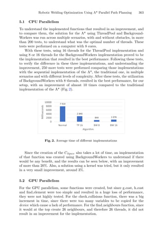

![Leaf-Based Species Recognition Using
Convolutional Neural Networks
Willian Oliveira Pires1
, Ricardo Corso Fernandes Jr.1
,
Pedro Luiz de Paula Filho1
, Arnaldo Candido Junior1(B)
,
and João Paulo Teixeira2
1
Federal University of Technology - Paraná, Medianeira Campus, Curitiba, Brazil
{willianpires,ricjun}@alunos.utfpr.edu.br, {plpf,arnaldoc}@utfpr.edu.br
2
Research Centre in Digitalization and Intelligent Robotics (CEDRI) – Instituto
Politecnico de Braganca, Braganca, Portugal
joaopt@ipb.pt
http://www.utfpr.edu.br/english, https://cedri.ipb.pt/
Abstract. Identifying plant species is an important activity in specie
control and preservation. The identification process is carried out mainly
by botanists, consisting of a comparison of already known specimens or
using the aid of books, manuals or identification keys. Artificial Neu-
ral Networks have been shown to perform well in classification problems
and are a suitable approach for species identification. This work uses
Convolutional Neural Networks to classify tree species by leaf images. In
total, 29 species were collected. This work analyzed two network mod-
els, Darknet-19 and GoogLeNet (Inception-v3), presenting a comparison
between them. The Darknet and GoogLeNet models achieved recognition
rates of 86.2% and 90.3%, respectively.
Keywords: Deep learning · Leaf recognition · Tree classification
1 Introduction
Sustainability is an important concern in the context of business and govern-
ments in view of nature preservation. According to Shrivastava [12], both busi-
nesses and governments play an important role in nature’s preservation. The
identification process of forest species is important in this context, specially in
the case of endangered species. Flora identification is currently made by botanists
by comparing with already known species or with book guidance, manuals and
identification keys. This comprises simple tasks as identifying whether the plant
have flowers and fruits to more complex tasks, such as identifying the plant
species by observing morphological attributes. For non-professionals, this pro-
cess can be long and error prone, so an automated tool would save time and,
possibly, plant species. The advancements made in computation, image process-
ing techniques and pattern recognition unveiled new ways of specie identification.
Deep learning based system are promising in this field, being helpful both for
the professionals and non-professionals.
c
Springer Nature Switzerland AG 2021
A. I. Pereira et al. (Eds.): OL2A 2021, CCIS 1488, pp. 367–380, 2021.
https://doi.org/10.1007/978-3-030-91885-9_27](https://image.slidesharecdn.com/optimizationlearningalgorithmsandapplications-231204021346-9e8015c0/85/Optimization-Learning-Algorithms-and-Applications-pdf-375-320.jpg)
![368 W. O. Pires et al.
In this work, we used leaf images to train Convolutional Neural Netowrks
(CNNs) for the classification task. Two models were trained: GoogLeNet
(Inception-v3) and Darknet-19, both implemented using Tensorflow. These mod-
els were chosen due to their light requirements when compared to other models,
allowing for use in low-cost equipment during field research. The models can be
used to identify species in natura.
This work is organized as follows. Section 2 presents an overview of CNNs,
specie identification and related works. Section 3 presents the materials and
methods used to train our models. Section 4 discusses the results. Finally, Sect. 5
contains the works conclusions.
2 Background
2.1 Species Identification
In order to realize plant species classification, botanists base themselves in veg-
etable taxonomy, analyzing characteristic group species by morphological simi-
larities and genetic kinship links [10]. This process generated a field in botany
called dendrology, which investigates woody plants identification, distribution
and classification [5]. Dendrology scope includes root types, tree sizes, pilosity,
shaft, as well as diagnostic elements (color, texture and structure). The shaft is
a tree trunk part free of ramifications which can be of different types, shapes
and bases.
Table 1 presents leaf components. The bases of leaf variety is its division type,
as there are simple leaves, which presents a single leaf lamina (Fig. 1). There are
also compound leaves, which present more than one leaflet, as shown in Fig. 2.
Table 1. Leaf Characteristics
Scientific name Description
Leaf venation Pattern of veins in the leaf
Hairiness Structures as hair in leaf surface
Leaf arrangement How leaves are arranged on a twig
Stem Plant structure that supports leaves, flowers and fruits
Stipule A pair of small organs that may be attached to the twig on
either side of the petiole
Leaf base Part of leaf nearest to the petiole
Leaf apexes Part of leaf farthest from petiole
Simple leaf Leaf that has a single blade
Compound leaf Leaf that has two or more blades that are called leaflets
Leaflets Leaf subdivisions that are related to compound leaf
Stalk A thin stem that supports a leaf and joints it to another part
of plant tree
Rachis Principal vein in the compound leaf, extension of stalk
Bud A small lump from which a flower, leaf or stem develops](https://image.slidesharecdn.com/optimizationlearningalgorithmsandapplications-231204021346-9e8015c0/85/Optimization-Learning-Algorithms-and-Applications-pdf-376-320.jpg)
![Leaf-Based Species Recognition Using Convolutional Neural Networks 369
Fig. 1. Simple leaf [5]
Fig. 2. Compound leaf [5]
There are other important leaf elements, which generate a wide specie vari-
ety, such as leaf shape, tip (or apex), base and margin attributes, which can
be used to differentiate plant species. Leafs also can be identified according to
their phyllotaxis, which are divided in four types: alternate, spiral, opposite and
whorled, shown in Fig. 3. This attribute is used before leaf extraction, as it shows
how leaves are organized. Other attribute is leaf venation, which is divided in
pinnate, reticulate, parallel, palmate and dichotomous (Fig. 4).
All those characteristics are taken in account during species identification
process and are the foundation of a widely used species identification method
among botanists: dichotomous key, which is based in plant characteristics obser-
vation. Researchers compare characteristics of field extracted species with the
characteristics of dichotomous keys, one by one, until matching with any of the
registered species [10]. Table 2 presents a simple example using a dichotomous
key to classify a leaf according to it’s venation.](https://image.slidesharecdn.com/optimizationlearningalgorithmsandapplications-231204021346-9e8015c0/85/Optimization-Learning-Algorithms-and-Applications-pdf-377-320.jpg)
![370 W. O. Pires et al.
Fig. 3. Leaf phyllotaxis [5]
Fig. 4. Leaf venation [5] onte
Table 2. Simple dichotomous key [5]
1. Leaves with a single vein and not ramified Single main vein
Leaves with more than a single venation 2
2. Leaves with more than a single vein and all
parallel between them
Parallel
Leaves with non-parallel veins 3
3. Secondary veins originates from a main vein Pinnate
Leaves with several main veins originating from
the petiole
Palmate
This is a fairly simple example, but in many cases characteristic selection
might not be trivial and plant specie identification will usually involve more than
a single characteristic. An example is Xanthosoma taioba, which is suitable for
consumption and hard to classify, as it is very similar to Xanthosoma violaceum,
which is not suitable for consumption. In Fig. 5, it becomes clear that differing
two species is not always a simple task.](https://image.slidesharecdn.com/optimizationlearningalgorithmsandapplications-231204021346-9e8015c0/85/Optimization-Learning-Algorithms-and-Applications-pdf-378-320.jpg)
![Leaf-Based Species Recognition Using Convolutional Neural Networks 371
Fig. 5. The real Xanthosoma taioba (right), and Xanthosoma violaceum (left) [5]
2.2 Convolutional Neural Networks
In the context of machine learning, specifically in neural networks, Convolu-
tional Neural Networks (CNNs) are a powerful model to analyze images. CNNs
are popular in image processing since they are inspired by the visual cortex.
These networks are based on the idea of specialized components inside a system
with specific tasks, in a similar fashion as the visual cortex observed by [16].
This architecture is composed by a sequence of layers that tries to capture a
hierarchy of increasingly sophisticated representations. Besides the input layer,
which normally consists of an image with width, height and color depth (RGB –
red, green and blue channels), there are three typical layers: convolution layer,
pooling layer and densely connected layer [15].
The first hidden layer in a CNN is usually a convolutional layer, which is
composed by many feature maps (filters), capable of learning patterns as the
training progresses [3]. Convolutional layers usually receive a two-dimensional
or a collection of input two-dimensional and are widely used to process images.
The layers are then submitted to a convolutional operation subject to parameters
learned during the network training phase.
Each layer usually also performs a non-linear operation which greatly
increases a model generalization capacity. This is done using an activation func-
tion. A popular function is the Rectified Linear Unit (ReLU), as it is a fast to
calculate non-linear function. It replaces negative input values by zero [15]. An
example as can be observed in (1), where z represents the function input (a
neuron input).
φ(z) =
0 z ≤ 0
z z 0
(1)
After a convolution and activation function, it is common the use of a pool-
ing layer. This technique aims to reduce the resulting matrix size, which dimin-
ishes the amount of neural network parameters to learn, contributing to avoid](https://image.slidesharecdn.com/optimizationlearningalgorithmsandapplications-231204021346-9e8015c0/85/Optimization-Learning-Algorithms-and-Applications-pdf-379-320.jpg)
![372 W. O. Pires et al.
overfitting [15]. Max pooling is a pooling technique in which several inputs close
to each other are replaced by a single value, the highest value in their neigh-
bourhood.
Each consecutive layer are capable of representing more complex concepts
than the previous layer. The last layers of a CNN usually are dense (or fully
connected) layers, built on top of the convolutional layers. In case of CNNs for
classification, the last layer outputs a n-dimensional vector, where n is the total
number of classes and each vector element is the predicted class probability
for one of the available classes [3]. For classification, it is common the use of
the Softmax function, which compares each output neuron response and return
the results in the form of probability. This function is presented in (2), for the
stimulus zj received by the j-nth output neuron.
φ(zj) =
ezj
k ezk
(2)
These models are normally trained using the Backpropagation and Gradi-
ent Descent algorithms. To avoid overfitting, dropout technique can be used.
Dropout approach consists on randomly removing neurons during training pro-
cess [1].
2.3 Darknet
Darknet is a neural topology usually implemented in the YOLO framework. This
framework allows real-time object detection and is able to identify objects in
images and videos as presented in Table 3. In this work, we investigated Darknet-
19, an architecture composed of 19 convolutional layers interspersed with 5 more
layers that apply max-pooling [3].
This network segments input image in SxS frames, known as grids. To do
this, it uses a divide and conquer strategy, making use of image segments to
identify object position in addition to only identifying objects [2].
2.4 GoogLeNet
GoogLeNet is a CNN that became notorious after winning the 2014 Imagenet
Competition. GoogLeNet engineer’s objective was to enhance neural network
computational efficiency while making it deeper and wider. The main feature in
GoogLeNet is the inception module, which is based on the idea of using multiple
convolutional filters [13] varying the kernel size used in the same convolutional
layer. The enhanced inception module is presented in Fig. 6.](https://image.slidesharecdn.com/optimizationlearningalgorithmsandapplications-231204021346-9e8015c0/85/Optimization-Learning-Algorithms-and-Applications-pdf-380-320.jpg)
![Leaf-Based Species Recognition Using Convolutional Neural Networks 373
Table 3. Darknet-19 [13]
Type Filters Stride/Size Output Dimension
Convolutional 32 3 × 3 224 × 224
Maxpool 2 × 2/2 112 × 112
Convolutional 64 3 × 3 112 × 112
Maxpool 2 × 2/2 56 × 56
Convolutional 128 3 × 3 56 × 56
Convolutional 64 1 × 1 56 × 56
Convolutional 128 3 × 3 56 × 56
Maxpool 2 × 2/2 28 × 28
Convolutional 256 3 × 3 28 × 28
Convolutional 128 1 × 1 28 × 28
Convolutional 256 3 × 3 28 × 28
Maxpool 2 × 2/2 14 × 14
Convolutional 512 3 × 3 14 × 14
Convolutional 256 1 × 1 14 × 14
Convolutional 512 3 × 3 14 × 14
Convolutional 512 3 × 3 14 × 14
Convolutional 256 1 × 1 14 × 14
Maxpool 2 × 2/2 7 × 7
Convolutional 1024 3 × 3 7 × 7
Convolutional 512 1 × 1 7 × 7
Convolutional 1024 3 × 3 7 × 7
Convolutional 512 1 × 1 7 × 7
Convolutional 1024 3 × 3 7 × 7
Convolutional 1000 1 × 1 7 × 7
Avgpool Global 1000
Softmax
GoogLeNet is a 22 layer network, considering only convolutional layers, as
shown in Table 4. The last layer uses the Softmax function to perform classifica-
tion [15].
2.5 Related Work
Many solutions based on deep learning have been used in specie identification
problems, due to recent results using this technique. Other strategies can also be
used, based on image processing and pattern recognition. These techniques use
macro and microscopic characteristics of the image. For example, [8] classifies
wood applying the following image characteristics extraction techniques: color](https://image.slidesharecdn.com/optimizationlearningalgorithmsandapplications-231204021346-9e8015c0/85/Optimization-Learning-Algorithms-and-Applications-pdf-381-320.jpg)
![374 W. O. Pires et al.
Fig. 6. Inception module [14]
Table 4. GoogLeNet’s structure [13]
Type Filters/Stride Output Dimension
Convolution 7 × 7/2 112 × 112 × 64
Max Pool 3 × 3/2 56 × 56 × 64
Convolution 3 × 3/1 56 × 56 × 192
Max Pool 3 × 3/2 28 × 28 × 192
Inception (3a) 28 × 28 × 256
Inception (3b) 28 × 28 × 480
Max Pool 3 × 3/2 14 × 14 × 480
Inception (4a) 14 × 14 × 512
Inception (4b) 14 × 14 × 512
Inception (4c) 14 × 14 × 512
Inception (4d) 14 × 14 × 512
Inception (4e) 14 × 14 × 832
Max Pool 3 × 3/2 7 × 7 × 832
Inception (5a) 7 × 7 × 832
Inception (5b) 7 × 7 × 1024
Avg Pool 7 × 7/1 1 × 1 × 1024
Dropout (40%) 1 × 1 × 1024
Linear 1 × 1 × 1000
Softmax 1 × 1 × 1000
analysis, GLCM (Gray-Leval Co-occurence Matrix), border histogram, fractals,
LBP (Local Binary Pattern), LPQ (Local Phase Quantization) and Gabor filter.
This approach resulted in a recognition rate of 99.49% among 42 species.
Another work with related theme proposes analysis and identification of plant
species based in texture characteristics extraction from microscopic leaf epider-
mis images [7]. Texture extraction techniques were used to analyze 32 species.
This approach had 96% success rate. By utilizing leaves, [11] applied image](https://image.slidesharecdn.com/optimizationlearningalgorithmsandapplications-231204021346-9e8015c0/85/Optimization-Learning-Algorithms-and-Applications-pdf-382-320.jpg)
![Leaf-Based Species Recognition Using Convolutional Neural Networks 375
segmentation techniques for feature extraction. This was performed using the
GLCM technique and feature vectors were extracted. The achieved recognition
rate was around 75.4% by techniques like MLP (Multilayer Perceptron), SMO
(Sequential Minimal Optimization) and LibSVM (Library for Support Vector
Machines) as classifiers.
Using deep learning as main identification method, the strategy is basically
to use CNNs to identify the best characteristic from the leaf to recognize a specie.
From this strategy, [6] build CNNs being used for weeds control, which tries to
detect a specie in the lawn. It was used 256 × 256 pixels images and the used
architecture was AlexNet. The result was 75% precision [9].
There are other CNN approaches, [17] proposes the analysis of pictures taken
from the top of farms, which demanded an extra detail preprocessing the image
to enhance illumination before sending it to the network, that is composed of
5 convolutional layers with ReLU activation function and, at the end of the
network, a Softmax function. Their experiment obtained 97.47% precision.
3 Method
3.1 Data Collection
Initially, leafs from 29 different species were collected. Species are listed in Sect. 4
(Table 4). For each species, 100 photos were taken on both sides. Images were
obtained through the utilization of a photobooth proposed by [11]. It has 40
square centimeters and its internal contains led strips, which produces high lumi-
nosity with low energy costs. These leds can be feed using batteries or a 12 V
power supply, and can be easily transported. To avoid reflexes on the images,
internal walls were painted black, except for the bottom, which is white. The
leaf is positioned on the bottom of the photobooth, where it is compressed by
a glass pane, to keep it fixed and flat. This dataset is in the process of being
public released.
After gathering enough photos, data augmentation techniques were used to
artificially increase dataset size, as it is necessary to have many samples to
train a Deep Neural Network. Data augmentation was done by using python
3.5.2 and Keras scripts to alter images, creating new ones. It was used Keras
ImageDataGenerator class to generate new image samples from the original data,
using the default values for the operations Rotation Range, Width Shift, Shear
Range, Zoom Range, Horizontal and vertical Flip and Fill mode.
3.2 Training
The models were then trained with the augmented data and had their results
evaluated, in order to improve performance. Both models, GoogLeNet and Dark-
Net19, were trained four times.
For GoogLeNet, we used the work of [13] as a reference to develop and train
our network. Originally, the network was developed with batch size of 50, Reduce
1 × 1 of 104 and Dropout rate of 0.5.](https://image.slidesharecdn.com/optimizationlearningalgorithmsandapplications-231204021346-9e8015c0/85/Optimization-Learning-Algorithms-and-Applications-pdf-383-320.jpg)
![376 W. O. Pires et al.
Regarding Darknet-19, we used the python implementation Darkflow, which
allow for the utilization of Darknet framework in Tensorflow [4]. Tiny-YOLO
version 2 was used instead of YOLO version 3, as it was faster to train. As
it was used 29 classes, the number of feature maps used in the last layer was
170, stride of size 1 and batch size of 64, following the default configuration for
Tiny-YOLO version 2.
4 Tests and Results
The original dataset were divided in 5,800 images for training and 580 for test.
In order to improve results, both sets were subject to augmentation, generating
34,800 images for training and 2,900 for test. The augmented dataset contains
independent training and test set, as no original image from training has an
augmented version in test. Similarly, augmented images in training has no version
in test.
Darknet model was first trained in the original dataset during 5.000 itera-
tions, presenting True Positive (TP) = 414, False Positive (FP) and False Neg-
ative (FN) of 166 and harmonic mean of 71.3%. After the first experiment, the
model was than trained over the augmented dataset, during 18,000 iterations.
Values presented by the network were TP = 2502, FP and FN of 398 and har-
monic mean of 86.2%. Precision and recall were calculated for each class. Results
are presented on Table 4 and Fig. 7.
GoogLeNet experiments were analogous for Darknet-19. First the model was
trained over the original dataset (5,800 images for training and 580 for test). This
process was performed for 2,000 iterations. The network presented TP = 461,
FP and FN of 119 and harmonic mean of 79.4%. For the second experiment,
(34,800 images for training and with 2,900 for validation) the iteration count
was raised to 4,000. The network presented the following values: TP = 2,633,
FP and FN of 267 and harmonic mean of 90.7%. Values for precision, recall and
harmonic mean were also calculated per class, presented on Table 4 and Fig. 8.
In the performed experiments, GoogLeNet had a better result than Darknet.
The difference between both networks in precision, recall and harmonic mean
were, respectively: 4.5, 4.8 and 4.7%. GoogLeNet results are good, even with a
broad and complicated dataset, as it were classified 29 classes, many of which
are similar.
Analyzing results with and without data augmentation, it became clear
the importance of a sufficient amount of data to work with CNNs. Differences
between Darknet and GoogLeNet trained with small and sufficient amount of
data was, respectively, 14.9% and 11.3%. The developed data augmentation algo-
rithm achieved it’s objective, expanding the dataset without damaging samples.](https://image.slidesharecdn.com/optimizationlearningalgorithmsandapplications-231204021346-9e8015c0/85/Optimization-Learning-Algorithms-and-Applications-pdf-384-320.jpg)
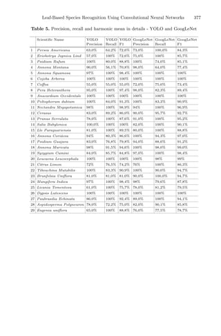
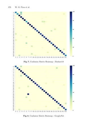
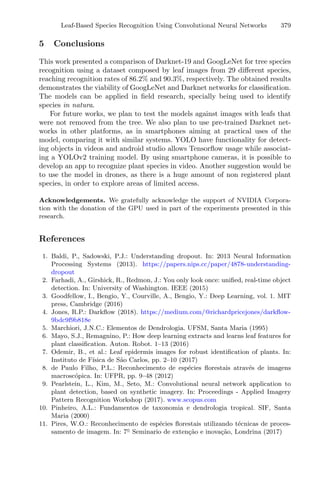

![Deep Learning Recognition of a Large
Number of Pollen Grain Types
Fernando C. Monteiro(B)
, Cristina M. Pinto, and José Rufino
Research Centre in Digitalization and Intelligent Robotics (CeDRI), Instituto
Politécnico de Bragança, Campus de Santa Apolónia, 5300-253 Bragança, Portugal
{monteiro,rufino}@ipb.pt
https://cedri.ipb.pt
Abstract. Pollen in honey reflects its botanical origin and melissopa-
lynology is used to identify origin, type and quantities of pollen grains
of the botanical species visited by bees. Automatic pollen counting and
classification can alleviate the problems of manual categorisation such as
subjectivity and time constraints. Despite the efforts made during the
last decades, the manual classification process is still predominant. One of
the reasons for that is the small number of types usually used in previous
studies. In this paper, we present a large study to automatically identify
pollen grains using nine state-of-the-art CNN techniques applied to the
recently published POLEN73S image dataset. We observe that existing
published approaches used original images without study the possible
biased recognition due to pollen’s background colour or using prepro-
cessing techniques. Our proposal manages to classify up to 97.4% of the
samples from the dataset with 73 different types of pollen. This result,
which surpasses previous attempts in number and difficulty of pollen
types under consideration, is an important step towards fully automatic
pollen recognition, even with a large number of pollen grain types.
Keywords: Pollen recognition · Convolutional neural network · Deep
learning · Image segmentation
1 Introduction
Food fraud has devastating consequences, particularly in the field of honey pro-
duction, which the U.S. Pharmacopeia Fraud Database1
has classified as the
third largest area of adulteration, only behind milk and olive oil. Our aim is to
find solutions to help solving this problem and prevent its recurrence. The deter-
mination of the botanical origin can be used to label honey and the knowledge
of the geographic origin is a factor that influences considerably the commercial
value of the product and can be used for quality control and to avoid fraud [6].
Although demanding, pollen grain identification and certification are crucial
tasks, accounting for a variety of questions like pollination or palaeobotany, but
1
https://decernis.com/solutions/food-fraud-database/.
c
Springer Nature Switzerland AG 2021
A. I. Pereira et al. (Eds.): OL2A 2021, CCIS 1488, pp. 381–392, 2021.
https://doi.org/10.1007/978-3-030-91885-9_28](https://image.slidesharecdn.com/optimizationlearningalgorithmsandapplications-231204021346-9e8015c0/85/Optimization-Learning-Algorithms-and-Applications-pdf-389-320.jpg)
![382 F. C. Monteiro et al.
also for other fields of research, including crime scene investigation [13], aller-
gology studies [7] as well as the botanical and geographical studies concerning
origins of honey to prevent honey labelling fraud [15]. However, most of the
pollen classification is a time consuming, laborious and a highly skilled work,
visually done by human operators using microscopes, trying to identify differ-
ences and similarities between pollen grains. These differences are, frequently,
imperceptible among pollen grains and may lead to identification errors.
Despite the efforts to develop approaches that allow the automatic iden-
tification of pollen grains [11,22], the discrimination of features performed by
qualified experts is still predominant [4]. Many industries, including medical,
pharmaceutical and honey marketing, depend on the accuracy of this manual
classification process, which is reported to be around 67% [19]. A notorious
paper [22] from 1996 published a brief summary of the state of the art until then
and, more importantly, the demands and needs of palynology to elevate the field
to a higher level, thus making it a more powerful and useful tool.
Pattern recognition from images has a long and successful history. In recent
years, deep learning, and in particular Convolutional Neural Networks (CNNs),
has become the dominant machine learning approach in the computer vision
field, specifically, in image classification and recognition tasks. Since the number
of annotated pollen images in the publicly available datasets is too small to train
a CNN from scratch, transfer learning can be employed. In this paper we pro-
pose an automatic pollen recognition approach divided into three steps: initially,
the regions which contain pollen are segmented from the background; then, the
colour is preprocessed; finally, the pollen is recognized using deep learning.
Most object recognition algorithms focus on recognizing the visual patterns
in the foreground region of the images. Some studies indicate that convolutional
neural networks (CNN) are biased towards textures [3], whereas another set of
studies suggests shape bias for a classification task [2]. However, little atten-
tion has been given to analyze how the recognition process is influenced by the
background information in the training process.
Considering that there are certain similarities between the layers of a trained
artificial network and the recognition task in the human visual cortex, in this
study, we hypothesize that if the collected images of a pollen have a unique
background colour, different from all the other pollens, it may biases the recog-
nition task, since the recognition could be based only in the background colour.
In order to study such influence we trained the CNN with several datasets:
one composed with original images, another composed with segmented images
(where the background colour was eliminated), and with preprocessed images
with histogram equalization and contrast limit adaptive histogram equalization
(CLAHE) techniques.
The acquisition of images usually has some different sources resulting in
images with different background, as shown in Fig. 1 from the POLEN73S2
dataset [1] used in this study. Deep learning based pollen recognition meth-
ods focus on learning visual features to distinguish different pollen grains. We
2
https://doi.org/10.6084/m9.figshare.12536573.v1.](https://image.slidesharecdn.com/optimizationlearningalgorithmsandapplications-231204021346-9e8015c0/85/Optimization-Learning-Algorithms-and-Applications-pdf-390-320.jpg)
![Deep Learning Recognition of a Large Number of Pollen Grain Types 383
observed that existing published approaches used the entire image with the orig-
inal background, in the training process. Background and foreground pixels in
each image contribute with the same influence into the learning algorithms. As
each pollen type has a different background from other types, when those trained
networks are used to classify the pollens they may be biased by capture relevance
from pollen’s background which may result in biased recognition.
Fig. 1. Pollen dataset samples acquired with different background colours.
In this paper, we investigate the background and colour preprocessing influ-
ence by training nine state-of-the-art deep learning convolutional neural net-
works for pollen recognition. We used a recently published POLEN73S image
dataset that includes more than three times as many pollen types and images as
the POLEN23E dataset used in recent studies. Our approach manages to classify
up to 97.4% of the samples from the dataset with 73 different types of pollen.
The remainder of this paper is organized as follows: Previous related works
are presented and reviewed in Sect. 2. In Sect. 3, we describe the used materials
and the proposed method. Section 4 presents the results and the discussion of
the findings. Finally, some conclusions are drawn in Sect. 5.
2 Related Works
Automatic and semi-automatic systems for pollen recognition based on image
features, in particular neural networks and support vector machines, have been
proposed for a long time [9,11,17,21]. In general terms, those approaches extract
some feature characteristics to identify each pollen type.
Although the classification remains based on a combination of image features,
the deep learning CNN approach builds a model determining and extracting
the features itself, in alternative of being predefined by human experts. Several](https://image.slidesharecdn.com/optimizationlearningalgorithmsandapplications-231204021346-9e8015c0/85/Optimization-Learning-Algorithms-and-Applications-pdf-391-320.jpg)
![384 F. C. Monteiro et al.
CNN learning techniques have been developed for classifying pollen grain images
[1,8,18,19]. In [8], Daood et al. present an approach that learns from the image
features and defines the model classifier from a deep learning neural network.
This method achieved a 94% classification rate on a dataset of 30 pollen types.
Sevillano and Aznarte in [18] and [19] proposed a pollen classification method
that applied transfer learning on the POLEN23E dataset and to a 46 different
pollen types dataset, achieving accuracies of over 95% and 98%, respectively. In
[1], Astolfi et al. presented the POLEN73S dataset and made an extensive study
with several CNNs, achieving an accuracy of 95.8%. Despite the importance of
their study, we identify two drawbacks in their approach, that influenced the
performance: they used different number of samples for each pollen type, and
used, for each pollen, an image background that is different from the image
background of other pollen types.
3 Experimental Setup
3.1 Pollen Dataset
The automation of pollen grain recognition depends on large image datasets with
many samples categorized by palynologists. The results obtained depend on the
number of pollen types and the number of samples used. Few samples may result
in poor learning models, that are not sufficient to train conveniently the CNN;
on the other hand, a small number of pollen types simplifies the identification
process making it impractical to be used for recognizing large numbers of pollens
usually found in a honey sample.
While a number of earlier datasets have been used for pollen grain classifi-
cation, such as the POLEN23E3
dataset [9] or the Pollen Grain Classification
Challenge dataset4
, which contain 805 (23 pollinic types) and 11.279 (4 pollinic
types) pollen images, respectively, in this paper we use POLLEN73S, which is
one of the largest publicly available datasets in terms of pollen types number.
POLLEN73S is an annotated public image dataset, for the Brazilian Savan-
nah pollen types. According to its description in [1] the dataset includes pollen
grain images taken with a digital microscope at different angles and manually
classified in 73 pollen types, containing 35 sample images for each pollen type,
except gomphrena sp, trema micrantha and zea mays, with 10, 34 and 29 sam-
ples, respectively. From the results presented in [1], we observed that these small
number of samples biased the results. Since CNNs were trained with a smaller
number of samples for those types of pollens, this resulted in the worst classifica-
tion scores relative to the other pollens. To overcome this problem, in our study,
several images were generated through rotating and scaling the original images
of these pollen types, ensuring the same number of samples for each pollen type,
which gives a total of 2555 pollen images. Although the images in the dataset
3
https://academictorrents.com/details/ee51ec7708b35b023caba4230c871ae1fa25
4ab3.
4
https://iplab.dmi.unict.it/pollenclassificationchallenge/.](https://image.slidesharecdn.com/optimizationlearningalgorithmsandapplications-231204021346-9e8015c0/85/Optimization-Learning-Algorithms-and-Applications-pdf-392-320.jpg)
![Deep Learning Recognition of a Large Number of Pollen Grain Types 385
have different width and height, they were resized accordingly with the image
size of each CNN architecture input.
More datasets were constructed by removing the pollen’s background colour
(see Fig. 2). Since the images background has medium contrast with the pollen
grains, the segmentation process uses just automatic thresholding and morpho-
logical operations. We also applied histogram equalization and contrast limit
adaptive histogram equalization (CLAHE) to those segmented images. These
new datasets allow the independence of training and testing processes from the
background colour among the pollen types.
Fig. 2. First column: original images; second column: segmented images with back-
ground colour removed; third column: segmented equalized images; fourth column:
segmented CLAHE images.
3.2 Convolutional Neural Networks Architectures
CNN is a type of deep learning model for processing images that is inspired by
the organization of the human visual cortex and is designed to automatically
create and learn feature hierarchies through back-propagation by using multiple
layer blocks, such as convolution layers, pooling layers, and fully connected layers
from low to high level patterns [2]. This technology is especially suited for image
processing, as it makes use of hidden layers to convolve the features with the](https://image.slidesharecdn.com/optimizationlearningalgorithmsandapplications-231204021346-9e8015c0/85/Optimization-Learning-Algorithms-and-Applications-pdf-393-320.jpg)
![386 F. C. Monteiro et al.
input data. The automatic extraction of the most discriminant features from a
set of training images, suppressing the need for preliminary feature extraction,
became the main strength of CNN approaches.
In this section, we present an overview of the main characteristics of the
CNNs used in this study for the recognition of pollen grains types. We choose
nine popular CNN architectures due to their performance on previous classifica-
tion tasks. Table 1 contains a list (chronological sorted) of state-of-the-art CNN
architectures, along with a high-level description of how the building blocks can
be combined and how the information moves throughout the architecture.
3.3 Transfer Learning
Constraints of practical nature, such as the limited size of training data, degrade
the performance of CNNs trained from scratch [18]. Since there is so much work
that has already been done on image recognition and classification [10,12,20], in
this study we used transfer learning to solve our problem. With transfer learning,
instead of starting the learning process from scratch, with a large number of
samples, we can use previous patterns that have been learned when solving a
similar classification problem.
Transfer learning is a technique whereby a CNN model is first trained on
a large image dataset with a similar goal to the problem that is being solved.
Several layers from the trained model, usually the lower layers, are then used in
a new CNN, trained with sampled images from the current task. This way, the
learned features in re-used layers are the starting points for the training process
and adapted to classify new types of objects. Transfer learning has the benefit of
reducing the training time for a CNN model and can overcome the generalization
error due to the small number of images used in the training process when using
a network from scratch.
The previous obtained weights, in each layer, may be used as the starting
values for the next layers and adapted in response to the new problem. This
usage treats transfer learning as a type of weight initialization scheme. This may
be useful when the first related problem has a lot more labelled data than the
problem of interest and the similarity in the structure of the problem may be
useful in both contexts.
3.4 Training Process
In the training process, the CNNs use the fine-tuning strategy, as well as the
stochastic gradient descent with momentum optimizer (SGDM) at their default
values, dropout rate set at 0.5 and early-stopping to prevent over-fitting, and
the learning rate at 0.0001. SGDM is used to accelerate gradients vectors in
the correct directions, as we do not need to check all the training examples
to have knowledge of the direction of decreasing slope, thus leading to faster
converging. Additionally, to consume less memory and train the CNNs faster,
we used the CNNs batch size at 12 to update the network weights more often,
and trained them in 30 epochs. All images go through a heavy data augmentation](https://image.slidesharecdn.com/optimizationlearningalgorithmsandapplications-231204021346-9e8015c0/85/Optimization-Learning-Algorithms-and-Applications-pdf-394-320.jpg)
![Deep Learning Recognition of a Large Number of Pollen Grain Types 387
Table 1. Chronological list and descriptions of CNN architectures used in this paper.
VGG 16/19 [20] Introduced the idea of using smaller filter kernels allowing
for deeper networks, and training these networks using pre-
training outputs of superficial layers. They have five convolu-
tional blocks where the first two have convolution layers and
one max-pooling layer in each block. The remaining three
blocks have three fully-connected layers equipped with the
rectification non-linearity (ReLU) and the final softmax layer
ResNet 50/101 [10] Shares some design similarities with the VGG architectures.
The batch normalization is used after each convolution layer
and before activation. These architectures introduce the
residual block that aims to solve the degradation problem
observed during network training. In the residual block, the
identity mapping is performed, creating the input for the next
non-linear layer, from the output of the previous layer
Inception-V3 [24] This network has three inception modules where the resulting
output of each module is the concatenation of the outputs
of three convolutional filters with different sizes. The goal
of these modules is to capture different visual patterns of
different sizes and approximate the optimal sparse structure.
Finally, before the final softmax layer, an auxiliary classifier
acts as a regularization layer
Inception-ResNet [23] Uses the combination of residual connections and the Incep-
tion architecture. In Inception networks the gradient is back-
propagated to earlier layers, and repeated multiplication may
make the gradient indefinitely small, so they replaced filter
concatenation stage with residual connections as in ResNet
Xception [5] The architecture is composed of three blocks, in a sequence,
where convolution, batch normalization, ReLU, and max
pooling operations are made. Besides, the residual connec-
tions between layers are made as in Resnet architecture
DenseNet201 [12] Is based on the ideas of ResNet, but built from dense blocks
and pooling operations, where each dense block is an iterative
concatenation from all previous layers. In the main blocks,
the layers are densely connected to each other. Massive reuse
of residual information allows for deep supervision as each
layer receives more information from the previous layer and
therefore the loss function will react accordingly, which makes
it a more powerful network
DarkNet53 [16] It has 53 layers deep and acts as a backbone for the YOLOv3
object detection approach. This network uses successive con-
volutional layers with some shortcut connections (introduced
by ResNet to help the activations propagate through deeper
layers without gradient vanishing) to improve the learning
ability. Batch Normalization is used to stabilize training,
speed up convergence, and regularize the model batch](https://image.slidesharecdn.com/optimizationlearningalgorithmsandapplications-231204021346-9e8015c0/85/Optimization-Learning-Algorithms-and-Applications-pdf-395-320.jpg)
![388 F. C. Monteiro et al.
which includes horizontal and vertical flipping, 360o
random rotation, rescaling
factor between 70% and 130%, and horizontal and vertical translations between
−20 and +20 pixels. The CNNs were trained using the Matconvnet package for
Matlab R
on a node of the CeDRI cluster with two NVIDIA RTX 2080 Ti GPUs.
As in [1], we used 5-Set Cross-Validation, where in each set the images were
split on two subsets, 70% (1825 images) for training and 30% (730 images) for
testing, allowing the CNN networks to be independently trained and tested on
different sets. Since each testing set is build with images not seen by the training
model, this allows us to anticipate the CNN behaviour against new images. The
four datasets (original, segmented, segmented with equalization and segmented
with CLAHE) were trained and tested in an independent way.
4 Results and Discussion
Other works use different evaluation metrics like Precision, Recall, F1-score [1]
or correct classification rate (CCR) [18]. However, those metrics use the concept
of true negative and false negative. As in this type of experiments we only obtain
true positives or false positives, we evaluate the results with Accuracy (Precision
gives the same score), which relates true positive with all possible results.
The evaluation results for the nine CNN architectures considered, with dif-
ferent colour pre-processing techniques, are presented in Table 2. The numbers
exhibited in bold indicate the best Accuracy result obtained for each network.
Table 2. Classification results (in percentage) on the test set for the different CNNs
and preprocessing techniques considered.
CNN Original Segmented Seg. Equal. Seg. CLAHE
VGG16 94.2 94.3 88.7 92.6
VGG19 91.9 92.4 92.1 92.1
ResNet50 95.1 95.2 93.2 94.8
ResNet101 94.5 94.6 93.0 95.2
Inception V3 92.3 92.8 94.0 90.8
Inception-ResNet 92.3 89.9 92.4 90.3
Xception 89.7 87.8 87.5 88.1
DenseNet201 96.7 97.4 96.6 95.9
DarkNet53 95.8 95.9 95.1 94.9
Based on the results of Table 2, we can conclude that segmenting pollen
grains images improves the classification performance for the majority of CNN
models allowing the DenseNet201 to achieve an accuracy of 97.4%. Only the
Xception network produces better results for the original images. The Inception
architectures achieve the best performance with segmented histogram equalized](https://image.slidesharecdn.com/optimizationlearningalgorithmsandapplications-231204021346-9e8015c0/85/Optimization-Learning-Algorithms-and-Applications-pdf-396-320.jpg)
![Deep Learning Recognition of a Large Number of Pollen Grain Types 389
images. The remain architectures achieved the highest performance when using
segmented images without any colour processing.
The DenseNet201 classified correctly all the images for 65 pollen grain types
out the 73 types of the dataset. For the other 9 types, it misclassified up to
two images, with a total of eleven false positives in the 730 tested images. The
lowest accuracy result of the DenseNet201 was achieved with the pollen types
dipteryx alata and myrcia guianensis. These pollen types have predominantly
rounded shapes and high texture, that are normally learned in the first CNN
layers. Since the transfer learning process changes only a set of the last CNN
layers it does not change those learned features during the training process with
our images, producing some misclassified results.
The accuracy rates achieved by the DenseNet201 network are relevant due to
the amount of pollen types in the POLEN73S dataset, since Sevillano et al. [19]
obtained a higher accuracy in a dataset containing only 46 pollen types. That
shows that DenseNet201 presented an important performance on POLEN73S.
The network trained and tested using the segmented images produced false
positives results that are misclassified as pollens that have high similarity with
the tested ones. Figure 3 shows some of those false positive examples.
Fig. 3. First row: segmented tested pollens (magnolia champaca, myrcia guianen-
sis, dipteryx alata, arachis sp); second row: misclassified pollens (ricinus communis,
schizolobium parahyba, zea mays, myracroduon urundeuva).
In networks trained and tested with segmented images the background colour
bias information was removed, and so the pollen is classified using only the grain
pollen information, correcting some of the false positives of the network trained
with original images, where the background colour was used as a feature in the
classification process.
The high values for the evaluation metric in all CNNs show that the number
of correctly identified pollens is high when compared to the number of tested](https://image.slidesharecdn.com/optimizationlearningalgorithmsandapplications-231204021346-9e8015c0/85/Optimization-Learning-Algorithms-and-Applications-pdf-397-320.jpg)
![390 F. C. Monteiro et al.
Table 3. Comparison with previous attempts at pollen classification of more than 20
pollen types using a CNN classifier, with number of types and the highest reported
accuracy.
Authors #Types Accuracy
Sevillano et al. [18] 23 97.2
Menad et al. [14] 23 95.0
Daood et al. [8] 30 94.0
Sevillano et al. [19] 46 97.8
Astolfi et al. [1] 73 95.8
Our approach 73 97.4
images. We believe that an accuracy over 97% is enough to build an automatic
classification system of pollen grains, since the visual classification performed by
human operators is a hard and time consuming task with a lower performance.
4.1 Comparison with Other Studies
We compared our results with other automatic approaches, from the current
literature, that used a CNN classifier. Previous deep learning approaches have
shown similar or higher accuracy rates to ours, but these studies were conducted
with a small number of pollen types. Table 3 provides a summary table of previ-
ous studies, including class sizes and accuracy/success rates against our result.
All the literature reviewed, except [1], used a significantly smaller image dataset,
in terms of pollen types, than the one used in this paper.
Although the work of Sevillano et al. [19], with forty six types of pollen,
achieved a slightly higher performance than our study, as the number of pollen
types is directly related to the classification performance of the CNNs, the results
must be evaluated taking into account this difference in the number of pollen
types between the work presented in [19] and ours.
In short, it can thus be concluded that training a network with the atten-
tion focused on the object itself by removing the background dissimilarities can
improve the performance of CNN model in pollen classification problem.
5 Conclusion
The usual method for pollen grains identification is a qualitative approach, based
on the discrimination of pollen grain characteristics by an human operator. Even
though this manual method is quite effective, the all process is time consuming,
laborious and sometimes subjective. Creating an automatic approach to identify
the grains, in a precise way, thus represents a task of utmost interest.
In this study, an automated pollen grain recognition approach is proposed.
We investigate the influence of background colours and colour pre-processing in](https://image.slidesharecdn.com/optimizationlearningalgorithmsandapplications-231204021346-9e8015c0/85/Optimization-Learning-Algorithms-and-Applications-pdf-398-320.jpg)
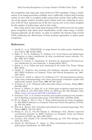

![Predicting Canine Hip Dysplasia
in X-Ray Images Using Deep Learning
Daniel Adorno Gomes1
, Maria Sofia Alves-Pimenta1,2
,
Mário Ginja1,2(B)
, and Vitor Filipe1,3
1
University of Trás-os-Montes and Alto Douro, 5000-801 Vila Real, Portugal
mginja@utad.pt
2
CITAB - Centre for the Research and Technology of Agro-Environmental
and Biological Sciences, Vila Real, Portugal
3
INESC TEC - INESC Technology and Science, 4200-465 Porto, Portugal
Abstract. Convolutional neural networks (CNN) and transfer learning
are receiving a lot of attention because of the positive results achieved
on image recognition and classification. Hip dysplasia is the most preva-
lent hereditary orthopedic disease in the dog. The definitive diagnosis is
using the hip radiographic image. This article compares the results of the
conventional canine hip dysplasia (CHD) classification by a radiologist
using the Fédération Cynologique Internationale criteria and the com-
puter image classification using the Inception-V3, Google’s pre-trained
CNN, combined with the transfer learning technique. The experiment’s
goal was to measure the accuracy of the model on classifying normal and
abnormal images, using a small dataset to train the model. The results
were satisfactory considering that, the developed model classified 75% of
the analyzed images correctly. However, some improvements are desired
and could be achieved in future works by developing a software to select
areas of interest from the hip joints and evaluating each hip individually.
Keywords: Canine hip dysplasia · CHD · Image recognition · CNN ·
Convolutional neural network · Artificial neural network ·
Inception-V3 · Artificial intelligence · Machine learning
1 Introduction
Canine hip dysplasia (CHD) is a hereditary disease that mainly affects dogs of
large and giant breeds [1]. The disease begins with pain and often the dog that
ran and jumped, cannot get up [2]. Genetic and environmental factors, such as
excessive growth rate, obesity, excessive and inadequate exercise can contribute
to the development of hip dysplasia in dogs [3]. The hip joint works like a ball
and a socket. Dogs with hip dysplasia develop osteoarthritis and the ball and
socket do not adjust [4]. Instead of sliding in a smooth way, they will rub and
grind, causing discomfort and gradually loss of function. Diagnostic radiography
is the main method used worldwide for screening hip dysplasia in dogs with
c
Springer Nature Switzerland AG 2021
A. I. Pereira et al. (Eds.): OL2A 2021, CCIS 1488, pp. 393–400, 2021.
https://doi.org/10.1007/978-3-030-91885-9_29](https://image.slidesharecdn.com/optimizationlearningalgorithmsandapplications-231204021346-9e8015c0/85/Optimization-Learning-Algorithms-and-Applications-pdf-401-320.jpg)
![394 D. A. Gomes et al.
breeding or management purposes [5]. Currently, radiographic analysis of CHD
is performed by veterinary radiologists using for scoring different schemes, of
which we highlight: the Fédération Cynologique Internationale’s (FCI) system
is most commonly used in continental European countries and uses five grades
(normal, borderline and three dysplastic grades); the Orthopaedic Foundation
for Animals (OFA) guidelines commonly used in the United States that uses
seven grades (three normal, borderline and three dysplastic); the British Veteri-
nary Association/Kennel Club scoring scheme is commonly used in the United
Kingdon and is a system that attributes disease points, the final dog’s score
ranges from 0 to 106 [4]. In general, all the schemes of assessment are consid-
ered subjective, and sometimes it is recommended the radiographic evaluation
by more than one examiner, being the agreement between the categories of dif-
ferent evaluators in the order of 50–60% [6]. Figure 1 shows examples of normal
(a) and CHD (b) X-ray images.
Fig. 1. Examples of normal (a) and CHD (b) X-ray images.
Advances in artificial intelligence, machine learning, image recognition and
classification, allied with the radiologic equipment, can be useful and help to
improve the diagnosis of this kind of disease. Convolutional Neural Networks
(CNN) are the architecture behind the most recent advances in computer vision.
They are currently providing solutions in many areas like image recognition,
speech recognition, and natural language processing. Through this program-
ming paradigm, a computer can learn from observational data. Practically, this
resource is allowing companies to create a wide range of applications like mecha-
nisms of autonomous vehicle vision, automatic inspection, anomaly detection in
medical imaging, facial recognition, for example, to unlock a mobile phone [7].
A CNN is a specific type of artificial neural network used mainly in image recog-
nition and natural language processing, also known as a ConvNet. The CNNs
combine deep learning algorithms and a multi-layer perceptron network that
consists of an input layer, an output layer and hidden layers that include convo-
lutional, normalization, pooling and fully connected layers, using mathematical](https://image.slidesharecdn.com/optimizationlearningalgorithmsandapplications-231204021346-9e8015c0/85/Optimization-Learning-Algorithms-and-Applications-pdf-402-320.jpg)
![Predicting Canine Hip Dysplasia in X-Ray Images Using Deep Learning 395
models to transmit the results to successive layers. The complexity of the objects
that a CNN can recognize increases accordingly with the filters learned by each
layer.
The first layers learn basic feature detection filters like corners and edges. The
middle layers learn filters that identify parts of objects—for dogs, for example,
they learn to recognize eyes, snouts, and noses. And, the last layers, learn to
identify complete objects, like to differentiate a dog from a cat or identifying
a dog’s race [8]. Pre-trained CNN such as AlexNet, VGGNet, Inception, and
Xception, allied with a technique called transfer learning, have been used to
build accurate models in a time saving way using small datasets [9]. The transfer
learning technique is a deep learning approach in which knowledge is transferred
from one model to another. When applying this technique it is possible to solve
a certain problem using all or part of a pre-trained model developed to solve a
different problem [10].
In this paper, the results of CHD scores attributed by a radiologist using
the FCI criteria were compared with the computer image classification using
the Inception-V3, Google’s pre-trained CNN [11], combined with the transfer
learning technique. The main aim of the work was to measure the accuracy of
the computer model on classifying normal and CHD images. Section 2 presents
the details on the materials and methods applied in the experiment. Section 3
shows the obtained results. Section 4 discusses the results and the performance
of the model, and make a few final remarks.
2 Methods
In this study, it was used a pre-trained network, the Google’s Inception-v3, that
was trained from the ImageNet database on more than a million images [12–14].
This CNN is 48 layers deep and can classify images into 1000 object categories
like chairs, pens, keyboards, animals, and cars. This network has an image input
size of 299 × 299 pixels. Figure 2 shows how the architecture of the Inception-V3
is structured.
The chosen pre-trained CNN, Inception-v3, was trained to identify charac-
teristics of normal and CHD in X-ray images. This new feature added a new
layer to the network capable of carrying out this type of identification. It is a
very popular technique called transfer learning, that permits to train a CNN on
a new task using a smaller number of training images. It consists of the reuse
of a pre-trained network as a starting point to learn about a new domain. The
rich feature representations already learned from a wide range of images and the
pre-trained layers are used to accelerate the process as the network will learn
new features creating the new layer [15]. In practice, this new layer will be the
last layer, and it will only be trained on the new domain to classify which X-ray
images are CHD positive or negative.
The dataset used in our experiments was provided by the Department of
Veterinary Science of the University of Trás-os-Montes and Alto Douro, Portugal.
It was used for training and testing the new layer of the CNN. The dataset](https://image.slidesharecdn.com/optimizationlearningalgorithmsandapplications-231204021346-9e8015c0/85/Optimization-Learning-Algorithms-and-Applications-pdf-403-320.jpg)
![396 D. A. Gomes et al.
Fig. 2. The architecture of the Inception V3. Extracted from [11].
contains a total of 225 X-ray digital images (1760X2140 pixels, 1-channel gray
scale, 8-bit depth in each channel, JPG format) obtained using the convenctional
ventro dorsal hip extended view. They were classified based on the FCI criteria
by a veterinary radiologist, 125 with hip dysplasia signs and 100 as normal.
The dataset was divided into 73% for the training (165 images) and 27% (60
images) for the test set, based on the protocol proposed in [16] that suggests
70% to train and 30% to test.
Table 1 shows how the dataset was structured to execute the training and
the test phases of the transfer learning process.
Table 1. Dataset split.
Type of image Training Test Total
Hip dysplasia 94 31 125
Normal 71 29 100
Total of images 165 60 225
The transfer learning technique was applied on the CNN using the Ten-
sorflow [17] deep learning framework and the Python programming language,
version 3.6. The model was trained and tested using a virtual machine created
on Oracle Virtual Box 5.2.2 and configured with Linux Mint 19.1 operating sys-
tem, an Intel(R) Core(TM) i7-5500U CPU @ 2.40 GHz processor, 8 GB of RAM
and an NVIDIA GeForce 920M GPU.
The total of iterations of the training process was 4000. It is the default
value defined by the Tensorflow framework. During the training process, three
metrics were used: the training accuracy, validation accuracy, and cross-entropy.
The training accuracy achieved was 100%. It represents the percentage of the
images used in the training process that were labeled with the correct category.
The cross-entropy is a loss function that represents the total loss minimization](https://image.slidesharecdn.com/optimizationlearningalgorithmsandapplications-231204021346-9e8015c0/85/Optimization-Learning-Algorithms-and-Applications-pdf-404-320.jpg)
![Predicting Canine Hip Dysplasia in X-Ray Images Using Deep Learning 397
during the training process. The total loss achieved a minimum of 0.038072. The
validation accuracy represents the percentage of images, randomly selected and
not used to train the model, that were correctly labeled. The validation accuracy
achieved was 83.8%. The final test accuracy achieved was 78.2%, meaning that
the model can make a correct prediction between 7 to 8 times out of 10.
After training the model with 165 images it was evaluated on the test set,
which includes 60 images unseen in the training phase. This is the classification
phase in which new samples are evaluated against the new model, and a predic-
tion is generated. Practically, it means that a script was executed for each of the
60 X-ray sample images to classify them in normal or CHD, based on the new
model. This script consists in a small program written in Python that executes
the process of classification in 5 steps. In the first step, it obtains the image that
will be classified. After, it loads the defined labels that will be used to classify
the images, in this case, normal and CHD. In the next step, it retrieves the
model generated in the training phase to compare to the new image, and finally,
provide a prediction.
The performance of the classification algorithm can be visualized in a confu-
sion matrix. Also, it is possible to calculate the accuracy of the algorithm through
Eq. 1, based on the values of the confusion matrix [18]. Both the performance
and the accuracy data will be shown in the results topic.
Accuracy = (TP + TN)/(TP + TN + FP + FN) (1)
3 Results
The confusion matrix in Fig. 3 was built from the model’s predictions obtained
on the test set.
Fig. 3. Obtained results applied in a confusion matrix.
The correct predictions are located in the diagonal of the table, highlighted
in yellow. The model classified correctly 26 images as CHD and 19 as normal. Of
the 31 actual CHD X-ray, the algorithm predicted that 5 were normal, and of the
29 normal, it predicted that 10 were CHD. Accordingly with the numbers of the
Fig. 3, the accuracy of the proposed model is (26+19)/(26+10+5+19) = 75%,](https://image.slidesharecdn.com/optimizationlearningalgorithmsandapplications-231204021346-9e8015c0/85/Optimization-Learning-Algorithms-and-Applications-pdf-405-320.jpg)
![398 D. A. Gomes et al.
considering the traditional default threshold of 0.5, due the binary nature of
the experiment [19]. In global, 45 X-ray images were classified with the correct
category, 26 representing animals with hip dysplasia and 19 with normal status.
The other 15 X-ray images evaluated in the test phase, were incorrectly
classified by the model, representing 10 normal animals and 5 with canine hip
dysplasia. In Fig. 4 are shown two X-ray image samples correctly classified by
the model.
Fig. 4. Samples correctly classified by the model in the test phase.
4 Discussion and Final Remarks
This paper presents a classification of canine X-ray images in hip dysplasia using
a pre-trained convolutional neural network combined with a transfer learning
technique. In part of the sample images, the algorithm used in this experiment](https://image.slidesharecdn.com/optimizationlearningalgorithmsandapplications-231204021346-9e8015c0/85/Optimization-Learning-Algorithms-and-Applications-pdf-406-320.jpg)

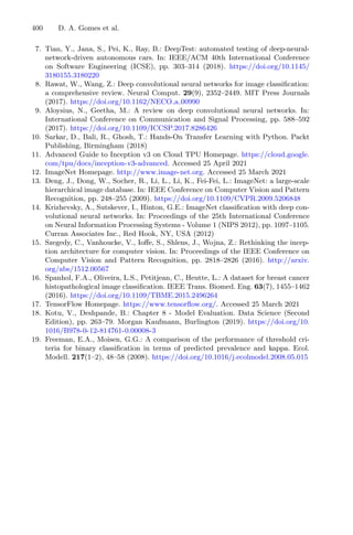
![Convergence of the Reinforcement
Learning Mechanism Applied to the
Channel Detection Sequence Problem
André Mendes(B)
Research Centre in Digitalization and Intelligent Robotics (CeDRI),
Polytechnic Institute of Bragança, 5300-253 Bragança, Portugal
a.chaves@ipb.pt
Abstract. The use of mechanisms based on artificial intelligence tech-
niques to perform dynamic learning has received much attention recently
and has been applied in solving many problems. However, the conver-
gence analysis of these mechanisms does not always receive the same
attention. In this paper, the convergence of the mechanism using rein-
forcement learning to determine the channel detection sequence in a
multi-channel, multi-user radio network is discussed and, through sim-
ulations, recommendations are presented for the proper choice of the
learning parameter set to improve the overall reward. Then, applying the
related set of parameters to the problem, the mechanism is compared to
other intuitive sorting mechanisms.
Keywords: Artificial intelligence · Reinforcement learning ·
Convergence analysis · Channel detection sequence problem
1 Introduction
The increasing use of devices that rely on wireless connections in unlicensed
frequency bands has caused huge competition for available spectrum. However,
studies conducted by regulatory agencies and universities show that the static
allocation currently practised through the sale of spectrum bands promotes, in
practice, the under-use of frequency bands, even in urban areas [1].
With this, the idea of dynamic access to spectrum [2] emerged as a solution
to improve the use of this scarce resource and thus provide alternative connec-
tivity for the growing demand-driven, for example, by the Internet of Things
devices. This dynamic access to spectrum relies on the use of devices whose
wireless network interface is reconfigurable, being able to dynamically adapt
their parameters and operating modes to the existing spectrum occupation.
Thus, considering a scenario of multiple frequency bands (called channels)
and users provided with a single transceiver, where only one channel can be
scanned at a time to detect possible “opportunities” for use and, in that same
time interval, effectively use the channel. In this scenario, the channel detection
c
Springer Nature Switzerland AG 2021
A. I. Pereira et al. (Eds.): OL2A 2021, CCIS 1488, pp. 401–416, 2021.
https://doi.org/10.1007/978-3-030-91885-9_30](https://image.slidesharecdn.com/optimizationlearningalgorithmsandapplications-231204021346-9e8015c0/85/Optimization-Learning-Algorithms-and-Applications-pdf-409-320.jpg)
![402 A. Mendes
sequence can have a major impact on user performance by minimising the time
to search and access a free channel.
When there is prior accurate knowledge of the channel statistics, the intuitive
detection sequence, the one that follows the decreasing sequence of channel avail-
ability probabilities is admittedly the optimal sequence [3]. However, in many
practical scenarios, the channel availability probability is unknown in advance,
and therefore, the optimal detection sequence requires a huge effort to obtain. A
first intuitive approach to solve this problem would be the historical observation
of this statistic, however, this approach would greatly increase the channel access
time due to the analysis required to obtain an accurate statistic.
Although the optimal stopping theory [4] combined with a brute-force mech-
anism can solve the problem, there is a strong dependency on previous and
accurate knowledge of the statistics of the channel and the computational cost
of this solution is high, growing even more with the increase of the number
of channels and users. Both problems impact directly the use of this solution
embedded in a platform with few resources.
In [5], the problem of choosing the channel detection sequence for only one
user was investigated and an approach was presented using a low computational
complexity method based on a reinforcement learning machine for the dynamic
search of the optimal detection sequence, where no prior knowledge of the avail-
ability probability and channel capacity is required.
In this paper, the evolution of the mechanism for searching the detection
sequence in a multi-channel, multi-user radio network using reinforcement learn-
ing, presented in [5], is discussed for the multi-user case, where the reward model
follows the optimal stopping theory [4]. The implementation of another strategy
for balancing the investigation-exploration dilemma is also included, and rec-
ommendations are presented for the choice of parameter ranges to improve the
overall reward of the mechanism. Then, the convergence analysis of the mech-
anism is performed by applying the aforementioned set of parameters to the
scenario. Finally, the results obtained are compared to those of other intuitive
sorting mechanisms.
This paper is organized as follows. Section 2 deals with related works.
Section 3 performs the summary of reinforcement learning, the adopted system
model and the proposal of the work that uses this technique for the search of
the optimal channel detection sequence. In Sect. 4, the simulation environment
is described, the convergence analysis of the mechanism is examined and the
results obtained are discussed. Finally, Sect. 5 concludes the paper and com-
ments on future work.
2 Related Work
The work in [6,7] obtains some empirical evidence describing the convergence
properties of reinforcement learning methods in multi-agent systems consider-
ing that in many practical applications it is not reasonable to assume that the
actions of other agents can be observed. Most agents interact with the surround-
ing environment relying on information from “sensors” because, without any](https://image.slidesharecdn.com/optimizationlearningalgorithmsandapplications-231204021346-9e8015c0/85/Optimization-Learning-Algorithms-and-Applications-pdf-410-320.jpg)
![Convergence of the RL Mechanism 403
knowledge of the actions (or rewards) of other agents, the problem becomes
even more complex.
In the work in [8], the authors studied the multiagent class of type indepen-
dent learners, including the convergence of the mechanism, in a deterministic
environment for some scenarios. In future work [9,10], the same class is studied
in a stochastic environment.
An important concept is that of regret (regret theory), which is defined as the
requirement where an agent obtains a reward that is at least as good as the one
obtained through any stationary strategy, independent of the strategy adopted
by the other agents [11]. For certain types of problems, the learning algorithms
that follow this concept converge to the optimal (Nash) equilibrium [12,13].
In the work presented in [14], the convergence of the class independent learn-
ers is established, while applied to the fictional player procedure [15] in com-
petitive games. Taking a differentiated approach, the work in [16] proposed an
algorithm of the class independent learners for repetitive games (where the player
is allowed to have a memory of past moves) that converges to a guaranteed fair
policy but periodically alternates between some equilibrium points.
3 Dynamic Channel Detection Sequence Using
Reinforcement Learning
The proposal of this work is a solution based on multi-agent reinforcement learn-
ing of the independent learners class using the Q-learning algorithm applied to
the problem of finding the optimal channel detection sequence in a network of
wireless devices. Using this approach it is optional to previous knowledge regard-
ing the probability of each channel to be available, nor the estimated quality of
each channel through its average SNRs (signal to noise ratios). Another impor-
tant advantage of this proposal is its adaptability to changes in channel charac-
teristics guaranteed by learning from the actions taken.
Therefore, the mechanism becomes immune to possible changes in the avail-
ability probabilities of the channels, which may occur due to changes in the pat-
terns of channel usage and possible changes in channel quality (average SNRs),
which may occur due to mobility and large scale fading effects.
From now on, the summary of the reinforcement learning technique will be
performed and, in the sequence, the modelling used for the search of the optimal
channel detection sequence will be described.
Reinforcement Learning
Reinforcement learning is one of the three paradigms in the field of artificial
intelligence, alongside supervised and unsupervised learning, where an agent
performs learning through observations of the results of its actions to maximise
a scalar value called reward (or reinforcement signal) [17].
When an agent acts, the obtained response (reward) does not contain infor-
mation about the correct action that should be taken. Rather, the agent needs](https://image.slidesharecdn.com/optimizationlearningalgorithmsandapplications-231204021346-9e8015c0/85/Optimization-Learning-Algorithms-and-Applications-pdf-411-320.jpg)
![404 A. Mendes
to discover for itself which actions lead to a greater reward by testing them. In
some interesting situations, actions may affect not only the immediate reward
but also those obtained in the future. The goal of the agent is to maximize the
sum of collected rewards.
The use of algorithms based on reinforcement learning, in particular, the Q-
learning [18], has received great attention lately. Being an algorithm that does
not need a model of the problem and capable of being used directly at runtime,
Q-learning is very suitable for application in systems with multiple agents, where
each agent has little knowledge of the others and where the scenario changes
during the learning period.
Q-learning adopts a simple approach, leading also to a low computational com-
plexity, which is important for platforms with few resources. In contrast, this
method can exhibit slow convergence [19].
The Q-learning algorithm works by estimating pair values (state, action)
from a value function Q, hence the name. The value Q(s, a), called Q-value,
is defined as the expected value of the sum of future rewards obtained by the
agent by taking the action a from the state s, according to an optimal policy
[18]. The agent initializes its Q-table with an arbitrary value and, at the instant
of choosing the action to be taken, a strategy is generally chosen in a way that
guarantees sufficient exploration while favouring actions with higher Q-values.
One commonly used strategy is the ε-greedy [17], which attempts to make
all actions, and their effects, equally experienced. In ε-greedy the agent uses the
probability given by ε to decide between exploring (exploitation) the Q-table or
investigating (exploration) randomly new states.
Another strategy is called softmax [17], where the probability of choosing a
particular action varies according to the corresponding value of Q-value. In this
strategy, a probability distribution is used for choosing an action a from a state
s. A commonly used distribution for this situation is the Boltzmann distribu-
tion. This distribution has a parameter, called temperature, which controls the
amount of exploration that will be practised. High values of temperature cause
an almost equiprobability of the choice of actions. Low values, on the contrary,
cause a great difference in the probability of choice of actions. In the limit, with
t → 0, the softmax strategy works as if it were the ε-greedy.
Qt+1(s, a) = Q(s, a) + α[r(s, a) + γmaxaQ(st+1, a) − Q(s, a)] (1)
In Q-learning, from the current state s, an action a is selected and subse-
quently a reward r is received, proceeding to the next state s
. With this, one
updates the value Q(s, a) according to Eq. 1, where α is the parameter called
learning rate and 0 ≤ γ ≤ 1 is the parameter called discount factor. Higher val-
ues of α indicate greater importance for present experience over history, while
higher values of γ indicate that the agent relies more on future reward than
immediate reward [20].
The Q-learning algorithm converges to the correct Q-values with probability
1 if and only if: the environment is stationary and Markovian, a storage table
is used to store the Q-values (usually named Q-table), no state-action pair is](https://image.slidesharecdn.com/optimizationlearningalgorithmsandapplications-231204021346-9e8015c0/85/Optimization-Learning-Algorithms-and-Applications-pdf-412-320.jpg)
![Convergence of the RL Mechanism 405
neglected (with time tending to infinity) and the learning rate is reduced appro-
priately with time [18]. The Q-learning does not specify which action should be
chosen at each step but requires that no action should fail to be tested.
System Model
In this work, each user was modelled as a learning agent following an indepen-
dent strategy according to the characteristics of the multi-agent class of type
independent learners [6]. This type of agent does not know the other agents,
interacting with the environment as if it were alone.
The agent, in this case, is unable to observe the rewards and actions of
the other agents and, consequently, can apply the Q-learning technique in its
traditional form. The choice of the multi-agent class, in particular, was motivated
by the possibility of future scalability of the mechanism by increasing the number
of agents and their autonomy, besides the enormous difficulty of satisfying, in
practice, the requirement of observation of the agents’ joint actions necessary
for the application of mechanisms of the joint learners class.
The system model adopted for the development and implementation of the
proposal allows the determination of the optimal detection sequence through the
application of the optimal stopping theory [5]. In this way, the goal is to provide
a decision about the moment to finalize the detection of new channels in such a
way that the reward obtained in the choice of a channel is maximized. This theory
then allows the definition of the stopping rule that maximizes the reward. The
optimal stopping theory provides a criterion for the choice of stopping (staying
on the free channel) or proceeding.
Consider a network with multiple users and a finite number of channels,
N. Each user is equipped with a transceiver for data exchange that can be
tuned to one of the N channels in the network. Moreover, each user has an
operating model whose access time, which we will call slot, devoted to channelling
observation and data transmission is constant with duration T.
In each slot, each channel i has the probability pi of being free or busy. It is
assumed that this probability is independent of its previous state and the state
of other channels, within each slot, and i.i.d. between slots.
Figure 1 exemplifies the activity of a user in a slot, which has two phases: a
detection phase and a data transmission phase. Before deciding to use a channel
in a given slot, the user must perform channel detection in the time equal to
τ to determine whether it is free or busy, minimizing the probabilities of non-
detection and false alarms.
In addition, the time equal to σ is reserved for channel probing, which has a
much shorter duration than the duration of the transmission phase, depends on
the channel bandwidth, modulation, etc., and whose result provides the trans-
mission rate that will be obtained, function of the momentary SNR of that user
on that channel. In the model, it is assumed that both channel detection and
channel probing are accurate and error-free tasks.](https://image.slidesharecdn.com/optimizationlearningalgorithmsandapplications-231204021346-9e8015c0/85/Optimization-Learning-Algorithms-and-Applications-pdf-413-320.jpg)
![406 A. Mendes
Fig. 1. Model of a slot.
Qt+1(s, a) =
(1 − α)Q(s, a) + α [r(s, a) + γmaxaQ(st+1, a)] if free channel
(1 − α)Q(s, a) + αγmaxaQ(st+1, a) if busy channel
(2)
Some constraints must be taken into account when taking actions and updat-
ing the Q-table, which is performed according to Eq. 2. One is that any action
taken in the state (ok, ∗), with 1 ≤ k ≤ (N − 1), always leads to a state where
the position in the detection sequence is ok+1. In the state where the position is
(oN , ∗), which represents the last channel in the detection sequence, the actions
indicate the first channel to be detected in the next slot, that is, it leads to
a state where the position in the detection sequence is (o1, ∗). When the user
decides to use a channel ci at position ok, the detection in that slot is terminated.
In that case, the first channel to be detected in the next slot will be determined
by the best action in state (oN , ci). Another important constraint is concerning
preventing the return to a previously detected channel (no recall).
The operation of the mechanism can be described as follows: at the beginning,
all state-action pairs of the Q-table are initialized with zeros. Then, the learning
phase begins, which is repeated during the entire period of the mechanism’s
operation. In this phase, the exploration strategy is chosen, whether softmax
or ε-greedy, and from it the action that will be followed from a given state is
chosen. After the execution of the action, the mechanism analyses if the channel
is free and decides whether to use it or not, continuing the detection according
to the established sequence of the channels. The goal is to provide a decision
about the moment to end the detection of new channels in such a way that the
reward obtained in choosing a channel is maximized. This indicates that it will
not always be advantageous to use the first free channel found.](https://image.slidesharecdn.com/optimizationlearningalgorithmsandapplications-231204021346-9e8015c0/85/Optimization-Learning-Algorithms-and-Applications-pdf-414-320.jpg)
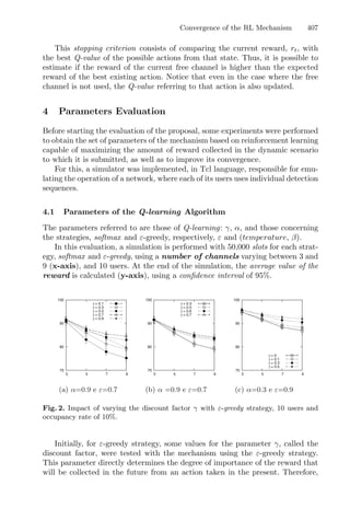
![408 A. Mendes
higher values of γ indicate that the agent relies more on the future reward than
the immediate reward
The results of this evaluation are shown in Fig. 2. For this analysis, it was
necessary to choose an initial range for the other parameters, α and ε, and our
choice was based on the values chosen for these same parameters previously [5].
It can be seen that the three approaches chosen (Figs. 2(a), 2(b) and 2(c)) point
to a relationship between the growth of γ and the increase in reward. However, it
can be noted that there is a threshold for the value of this parameter, between 0.7
and 0.9, which reverses the trend (Fig. 2(a)). An observation of the behaviour of
the parameter for values closer to 0.7 (Fig. 2(b)) demonstrates that the collected
reward values can be considered equal, due to the confidence interval, if γ is
in the interval [0.5, 0.7]. We opted for the smaller value as it favours a fast
convergence of the mechanism [17] .
70
80
90
100
3 5 7 9
α = 0.1
α = 0.3
α = 0.5
α = 0.7
α = 0.9
(a) γ = 0.5 e ε = 0.7
70
80
90
100
3 5 7 9
α = 0.1
α = 0.3
α = 0.5
α = 0.7
α = 0.9
(b) γ = 0 e ε = 0.7
84
86
88
90
92
94
96
98
100
3 5 7 9
ε = 0.1
ε = 0.5
ε = 0.7
ε = 0.9
ε = 1.0
(c) γ = 0.5 e α = 0.1
84
86
88
90
92
94
96
98
100
3 5 7 9
ε = 0.9
ε = 0.95
ε = 1
(d) γ = 0 e α = 0.3
Fig. 3. Impact of varying the learning rate α and the parameter ε with ε-greedy strat-
egy, 10 users and occupancy rate of 10%.
Then, the impact of varying the parameters α and ε was verified (Fig. 3).
Initially, the parameter α, called learning rate, was analysed. Briefly, larger val-
ues of this parameter benefit recent experience against the historical experiences
(or acquired knowledge) of the mechanism. In the same way, as in the previous
analysis, it was necessary to choose the initial value of the other parameters, γ
and ε. The γ value was obtained previously and the ε value was chosen as 0.7.
As can be seen in Figs. 3(a) and 3(b), smaller values of α provide better per-
formance of the mechanism. It was expected that this result would demonstrate
the importance of adapting the mechanism to the dynamics of the environment
and how much this would influence the overall performance, however, it was
found that it is more important to value the acquired knowledge, keeping the
parameter α low.
The parameter ε, also called exploration level, is linked to the ε-greedy strat-
egy and establishes the probability that directs the mechanism to explore new
states. The appropriate choice in the expose level depends very much on the
problem to be addressed. If the purpose of the problem requires intense learn-
ing, the value of this parameter tends to be higher. On the other hand, if in the
problem there is the execution of other tasks parallel to the learning, it does not](https://image.slidesharecdn.com/optimizationlearningalgorithmsandapplications-231204021346-9e8015c0/85/Optimization-Learning-Algorithms-and-Applications-pdf-416-320.jpg)
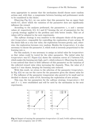
![410 A. Mendes
4.2 Number of Users and Channel Occupancy
In this part, an experiment is carried out to determine the impact of varying
the number of users simultaneously with the variation of the channel occupancy.
The purpose is to evaluate the importance of using a mechanism adaptable
to the increase in the number of users, independent of the channel occupancy.
Moreover, with the increase of the number of slots the values of the collected
reward (y-axis) can be observed and conclusions about the convergence of the
mechanism can be drawn.
In this experiment, a simulation is performed with 100,000 slots for each strat-
egy, softmax and ε-greedy, using a number of channels equal to 9. The number
of channels was chosen assuming that there will be greater “opportunities” for
users as there are more channels. The plotted figures have been harvested at
20% of the total number of slots to take advantage of the part that contains the
most information.
0
20
40
60
80
100
10 20 30 50 100
Slot [x 100]
1 US
10 USs
15 USs
20 USs
(a) Occupancy =
10%, softmax
0
20
40
60
80
100
10 20 30 50 100
Slot [x 100]
1 US
10 USs
15 USs
20 USs
(b) Occupancy =
90%, softmax
0
20
40
60
80
100
10 20 30 50 100
Slot [x 100]
1 US
10 USs
15 USs
20 USs
(c) Occupancy =
10%
0
20
40
60
80
100
10 20 30 50 100
Slot [x 100]
1 US
10 USs
15 USs
20 USs
(d) Occupancy =
90%
Fig. 5. Impact of varying the number of users and the channel occupancy parameter
for both strategies and with 9 channels.
The results of this examination are shown in Fig. 5. As expected, it is pos-
sible to observe that with low channel occupancy the obtained reward values
are higher (Figs. 5(b) and 5(d)), a direct consequence of the higher amount of
“opportunities” for the users. In this result, it is also possible to observe that
there is a better performance of the mechanism for a certain number of users,
in both strategies. It is possible to understand this phenomenon as a result of
the users’ accommodation, a consequence of the greater dispute for the available
opportunities, which are not enough for the demand, causing a reduction in the
reward when the number of users increases too much.
When the channel occupancy parameter increases, a reduction in the reward
values are expected, which can be seen in Figs. 5(a) and 5(c). In this scenario, it
is also noted that there is a better performance of the mechanism for a certain
number of users, although the value is different from that present when there
are more “opportunities” available.
Another important observation is that the ε-greedy strategy outperforms soft-
max when applied to the problem, regardless of the channel occupancy rate. This](https://image.slidesharecdn.com/optimizationlearningalgorithmsandapplications-231204021346-9e8015c0/85/Optimization-Learning-Algorithms-and-Applications-pdf-418-320.jpg)
![Convergence of the RL Mechanism 411
somewhat contradicts the theory that there is a predominance of the softmax
technique, demonstrating that in certain scenarios and applications, the ε-greedy
technique can indeed have superior performance [17].
The results obtained with this experiment also point to a need for adaptation
of the mechanism to the number of users, being interesting that should be a
capability of autonomous restriction of this quantity by the mechanism, aiming
to reach a bigger reward. This will be investigated in future works.
Regarding the convergence of the mechanism, even with the significant
increase in the number of channels, the mechanism shows to be robust, evolving
through a transitory period until the convergence in an equilibrium point, as the
number of slots increases.
4.3 Number of Channels and Channel Occupancy
In this part, the effects on the reward (y-axis) due to the variation of the num-
ber of channels simultaneously with the variation of the channel occupancy were
evaluated. For this purpose, a similar experiment to the previous one (Sect. 4.2)
was carried out, starting from a simulation with the same amount of slots for
each strategy, softmax and ε-greedy. A total of 10 users were used, as per the
results obtained in Sect. 4.2. Plotted figures were harvested at 20% of the total
number of slots for clarity, as in the previous analysis.
As expected, for both strategies and the two evaluated rates of the chan-
nel occupancy parameter, the highest reward values were obtained with the
highest channel offer (Fig. 6). However, with low channel availability for users
(Figs. 6(a) and 6(c)), the performance of the mechanism was similar for 3 chan-
nels or 5 channels. The cause of this behaviour is that a high rate of the channel
occupancy parameter with a reduced number of channels means that there are
fewer “opportunities” to be taken advantage of by the mechanism, and a small
increase in these “opportunities” is enough for the mechanism performance to
raise significantly.
0
20
40
60
80
100
10 20 30 50 100
Slot [x 100]
3 channels
5 channels
9 channels
(a) Occupancy =
10%, softmax
0
20
40
60
80
100
10 20 30 50 100
Slot [x 100]
3 channels
5 channels
9 channels
(b) Occupancy =
90%, softmax
0
20
40
60
80
100
10 20 30 50 100
Slot [x 100]
3 channels
5 channels
9 channels
(c) Occupancy =
10%
0
20
40
60
80
100
10 20 30 50 100
Slot [x 100]
3 channels
5 channels
9 channels
(d) Occupancy =
90%
Fig. 6. Impact of varying the number of channels and the channel occupancy parameter
with both strategies, for 10 users.
For all the configurations presented, it was shown that the mechanism is
immune to any perturbation caused by the variation, either of the number of](https://image.slidesharecdn.com/optimizationlearningalgorithmsandapplications-231204021346-9e8015c0/85/Optimization-Learning-Algorithms-and-Applications-pdf-419-320.jpg)
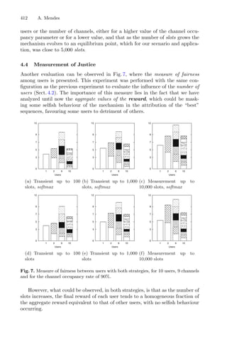
![Convergence of the RL Mechanism 413
This result also contributes to strengthening the hypothesis that the mecha-
nism converges to an equilibrium point since at this point the individual strate-
gies do not lead to the greedy behaviour of some users.
4.5 Results
To evaluate the performance of the proposal, the developed simulator was
extended and the following detection sequences were evaluated:
– the dynamic sequence of the channels provided by the mechanism (RL);
– the sequence of channels in the decreasing sequence of their availability prob-
abilities (Prob);
– the sequence given by the descending sequence of the average capacities of
each channel (CAP) [3]; and,
– the random sequence of channels (RND).
It is worth noting that all of the evaluated sequences, except the RL sequence,
are static, i.e., they do not change throughout the simulation. In the case of
the sequence RL, due to reinforcement learning itself, the sequence may vary
during the simulation. Moreover, all sequences, except for the RL and the RND,
assume a priori knowledge of the average capacities of each channel and/or their
availability probabilities.
At the beginning of each simulation round, the value of the average capac-
ity and availability probabilities of each channel i, i ∈ 1, ..., N, were drawn.
The availability probability of each channel is drawn uniformly within the
interval [0, 1]. The average capacity is drawn following a uniform distribu-
tion within the interval [0.1 × CAPMAX, CAPMAX], where CAPMAX is
the maximum average capacity of the channels. And the instantaneous capac-
ity of each channel is drawn using a uniform distribution within the interval
[0.2×CAPMEDIA, CAPMEDIA], where CAPMEDIA is the average capac-
ity of each channel.
Channel occupancy modelling was established according to an exponential
on-off model synchronised with the slots. With this, a given channel remained
in the occupied state for a period equal to tOF F equivalent to the mean of
an exponential distribution. Thus, tON can be obtained by tON = (1−u)×tOF F
u ,
where u is the channel occupancy rate.
The value of Wm, referring to the collision probability, was set to 8 [21].
Thirty rounds of the simulation were performed for each set of parameters. In
all simulations, CAPMAX was configured with a fixed value of 10 and the size
of the slot was configured as variable, with a value equal to twice the number of
channels used in the simulation multiplied by τ.
The metric used for evaluation was the reward obtained by each of the
sequences implemented using the same states and instantaneous channel capac-
ities (fairness criterion) at each slot, corresponding to the effective transmission
rate obtained by the user when using the channel (Sect. 3) and calculated by the
simulator, at the end of each round, as the average reward obtained by each of](https://image.slidesharecdn.com/optimizationlearningalgorithmsandapplications-231204021346-9e8015c0/85/Optimization-Learning-Algorithms-and-Applications-pdf-421-320.jpg)
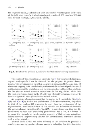
![Convergence of the RL Mechanism 415
ration threshold of the available capacity of the network according to the number
of available channels.
From Figs. 8(c) and 8(g), it can be seen that with few users, the reward
obtained varies little with the variation of occupancy (x-axis) and channels.
When the number of users increases (Figs. 8(d) and 8(h)), an increase in reward is
observed, although it can be noted that the variation in the parameter occupancy
is small, maintaining a similar percentage growth of reward with the increase in
the number of available channels.
Finally, the ε-greedy strategy had a superior result than the softmax strat-
egy, when applied to the problem. A possible explanation for this lies in the fact
that when Q-learning is used in modelling with a high number of actions, it is
expected to observe a high number of overestimations, which impair the perfor-
mance of the strategy, in some of the values of the actions if there is some noise
in these values, for example, due to the use of approximate value functions or
too abrupt transitions between states. Another explanation comes from the fact
that for some applications/modelling, the softmax strategy keeps exploring for
a long time, oscillating between many actions that obtain rewards with similar
values, also harming its performance [22].
5 Conclusions and Future Works
In this paper, the evolution of the mechanism presented in [5] is discussed for
the multi-user case. The implementation of the softmax strategy to balance the
research-exploration dilemma is also included along with recommendations for
the choice of parameters to improve the overall reward. Then, the convergence
of the mechanism is verified by applying the aforementioned set of parameters.
Finally, the performance evaluation of the evolved mechanism is performed.
Actually, the proper selection of a set of parameters for the mechanism allows
maximizing the reward (data throughput). However, its performance is strictly
related to the values chosen and, hence, the state of the RF environment could
degrade the performance.
It is always worth noting that RF communication is widely used in practical
applications, e.g. for the gathering of data from sensors spread over a primary
production area (agriculture).
As future works, we have the investigation of optimal values for the parame-
ters, the implementation of new strategy to balance the exploitation-exploration
dilemma and the evolution of the mechanism for autonomous user control in
order to achieve a higher reward, as shown in Sect. 4.2.
Acknowledgements. This work has been conducted under the project “BIOMA
– Bioeconomy integrated solutions for the mobilization of the Agri-food market”
(POCI-01-0247-FEDER-046112), by “BIOMA” Consortium, and financed by European
Regional Development Fund (FEDER), through the Incentive System to Research and
Technological development, within the Portugal2020 Competitiveness and Internation-
alization Operational Program.](https://image.slidesharecdn.com/optimizationlearningalgorithmsandapplications-231204021346-9e8015c0/85/Optimization-Learning-Algorithms-and-Applications-pdf-423-320.jpg)

![Approaches to Classify Knee
Osteoarthritis Using Biomechanical Data
Tiago Franco1(B)
, P. R. Henriques2
, P. Alves1
,
and M. J. Varanda Pereira1
1
Research Centre in Digitalization and Intelligent Robotics,
Polytechnic Institute of Bragança, Bragança, Portugal
{tiagofranco,palves,mjoao}@ipb.pt
2
ALGORITMI Centre, Department of Informatics,
University of Minho, Braga, Portugal
prh@di.uminho.pt
Abstract. Knee osteoarthritis (KOA) is a degenerative disease that
mainly affects the elderly. The development of this disease is associ-
ated with a complex set of factors that cause abnormalities in motor
functions. The purpose of this review is to understand the composition
of works that combine biomechanical data and machine learning tech-
niques to classify KOA progress. This study was based on research arti-
cles found in the search engines Scopus and PubMed between January
2010 and April 2021. The results were divided into data acquisition, fea-
ture engineering, and algorithms to synthesize the discovered content.
Several approaches have been found for KOA classification with signifi-
cant accuracy, with an average of 86% overall and three papers reaching
100%; that is, they did not fail once in their tests. The acquisition of data
proved to be the divergent task between the works, the most considerable
correlation in this stage was the use of the ground reaction force (GRF)
sensor. Although three studies reached 100% in the classification, two did
not use a gradual evaluation scale, classifying between KOA or healthy
individuals. Thus, we can get out of this work that machine learning
techniques are promising for identifying KOA using biomechanical data.
However, the classification of pathological stages is a complex problem
to discuss, mainly due to the difficult access and lack of standardization
in data acquisition.
Keywords: Knee osteoarthritis · Biomechanical · Data classification ·
Machine learning
1 Introduction
Osteoarthritis (OA), the most common form of arthritis, is a degenerative joint
disease caused by rupture and eventual loss of the cartilage that lines the bony
extremities [18]. This disease is directly related to aging and usually affects the
knee, hip, spine, big toe, and hands. Estimates show that about 10% of men and
c
Springer Nature Switzerland AG 2021
A. I. Pereira et al. (Eds.): OL2A 2021, CCIS 1488, pp. 417–429, 2021.
https://doi.org/10.1007/978-3-030-91885-9_31](https://image.slidesharecdn.com/optimizationlearningalgorithmsandapplications-231204021346-9e8015c0/85/Optimization-Learning-Algorithms-and-Applications-pdf-425-320.jpg)
![418 T. Franco et al.
18% of women over 60 years of age have some kind of the OA, reinforcing its
worldwide importance in public health [17].
In particular, knee osteoarthritis (KOA) is the type of OA with the highest
perceived prevalence. The most characteristic symptoms of KOA are usually
changing in biomechanical behavior, such as joint pain, stiffness, cracking, and
locking of the joints. These symptoms are typically noticed earlier because they
interfere with daily activities, especially gait abnormalities [21].
The development of KOA is associated with a combination of a complex set
of factors. These risk factors can be divide into non-modifiable and modifiable,
including joint integrity, genetic predisposition, local inflammation, mechanical
forces, and cellular and biochemical processes. Consequently, several treatments
have been creating to improve motor function, relieve pain, and alleviate the
deficiencies caused [10].
One of the fundamental pieces for developing a sophisticated treatment is
the understanding and classification of the progression of KOA. As this infor-
mation becomes more practical and accessible, more realistic monitoring of the
case becomes possible, enabling the physiotherapist to prepare a more efficient
specialized solution [2]. In addition, it also creates the possibility of expanding
the early detection of KOA, reducing the prevalence of the disease in the global
population [3].
The most common techniques used to classify KOA progression are X-rays
and magnetic resonance imaging (MRI). Unfortunately, both have limitations;
radiography is low-priced but is generally low-resolution and used only for initial
evaluation. The MRI has better accuracy and is helpful for monitoring stages
of the pathology, but it is expensive [2]. In addition, patients generally seek
these techniques after feeling uncomfortable, making it challenging to detect
asymptomatic patients early.
Thus, researchers from different areas seek to propose innovative, low-cost,
and scalable solutions for OA. The application of computational techniques,
mainly machine learning, stands out to be constantly growing and orthogonal to
most adjacent areas. The evolution of the data acquisition and analysis capacity
aroused great interest from the scientific community, enabling new automated
solutions for pre or post treatment [5].
As a result, several clinical and observational databases are being created,
analyzed, and made available online. These data are highly dimensional, hetero-
geneous, and voluminous, opening up a new range of possibilities and challenges
for improving KOA diagnosis [14].
Studies show evidence that it is possible to recognize through biomechanical
data, including kinematic-kinetic data and electromyography (EMG) signals, the
difference in the behavior of patients with KOA and pathological stage indica-
tions [1,17]. In addition, the review about the application of machine learning
in KOA developed by Kokkotis et at. [5], shows that the application of ML
algorithms for KOA classification using biomechanical data performs similarly
to models built on image data (x-rays and MRI).](https://image.slidesharecdn.com/optimizationlearningalgorithmsandapplications-231204021346-9e8015c0/85/Optimization-Learning-Algorithms-and-Applications-pdf-426-320.jpg)
![Approaches to Classify Knee Osteoarthritis Using Biomechanical Data 419
That said, there was a desire to understand in more detail the composi-
tion of works that focus on biomechanical data, identifying and categorizing
the most common and promising forms of data acquisition, resource engineering
and algorithms. Thus, the present work reviews the literature with the purpose
of systematizing and comparing the knowledge produced by articles that use
biomechanical data to classify the KOA through machine learning algorithms.
The paper is organized in four more sections after this one. Section 2 refers to
the methodology used, such as keywords and selection criteria; Sect. 3 compiles
the results of this article, describing the relevant points found in the reviewed
articles on data acquisition, resource engineering and algorithms; Sect. 4 dis-
cusses the results and the points that we believe should be highlighted; Sect. 5
reports the main conclusions and scientific contributions that we have drawn
from this study.
2 Methods
The literature review presented summarizes the works found in the Scopus and
PubMed repositories. Several combinations of keywords were used in the search,
with the most recurring ones: biomechanical, gait, machine learning, deep learn-
ing, classification, osteoarthritis. Searches were limited by the year of publication
between January 2010 and April 2021.
The focus of the review is to find articles that use biomechanical data from
patients with KOA. Therefore, three rules were used to define the inclusion
criteria, namely:
1. Only articles that mention clinical evidence of the presence of KOA in patients
included in the study;
2. Only articles that handle with biomechanical data;
3. Studies that propose to classify KOA using machine learning algorithms.
For the exclusion criteria, only two rules were added, namely:
1. Studies did not specify KOA as the presenting pathology;
2. Studies that used analytical methods for KOA classification.
Two review papers inspire this study with correlated objectives. The review
[5] synthesizes machine learning techniques in diagnosing knee osteoarthritis
between 2006 to 2019. The study comprehensively explores using any data
applied to knee osteoarthritis, including MRI, X-Ray, Kinetic and Kinematic
data, Clinical data, and Demographics. The second review mentioned [8] makes
a survey on the evaluation of knee osteoarthritis based on gait between 2000
to 2018. The study shows to be the most comprehensive on the subject by dis-
cussing in detail the various techniques applied to the understanding of human
gait and its difference for KOA patients.
The present study differs from the ones mentioned, being more specific,
including only works that use Kinetic and Kinematic data for the classifica-
tion of knee osteoarthritis through machine learning techniques. The focus of
this work is to detail the construction of the dataset and explore the different
models based on the biomechanical data.](https://image.slidesharecdn.com/optimizationlearningalgorithmsandapplications-231204021346-9e8015c0/85/Optimization-Learning-Algorithms-and-Applications-pdf-427-320.jpg)
![420 T. Franco et al.
3 Results
Twelve articles were selected according to the criteria described to be explored.
A list with the meta-information can be seen in Table 1.
Table 1. Selected articles
Index Author Year Country Repository
1 Köktaş [22] 2010 Turkey Scopus
2 Moustakidis [15] 2010 Greece Scopus
3 McBride [12] 2011 USA Scopus
4 Kotti [6] 2014 UK PubMed
5 Phinyomark [19] 2016 Canada PubMed
6 Kotti [7] 2017 UK Scopus
7 Muñoz-Organero [16] 2017 China Scopus
8 Long [11] 2017 UK Scopus
9 Mezghani [13] 2017 Canada Scopus
10 Kobsar [4] 2017 Canada PubMed
11 Kwon [9] 2020 Korea PubMed
12 Vijayvargiya [20] 2020 India Scopus
Two-thirds of the articles found are available on Scopus, with the majority of
the articles being after 2015, with the highest concentration in 2017 with 05/12.
In addition, it was also noted that there is a correlation of authors between the
articles Kotti [6,7] and Long [11], as well as Phinyomark [19], Mezghani [13] and,
Kobsar [4].
N. Kour [8] describes that the pipeline commonly followed to classify KOA
using computable data has five main stages, illustrated in Fig. 1. The first step
is to acquire data from KOA patients and healthy individuals; the second step
is pre-processing, where techniques are applied to improve the quality of the
data; the third phase is the extraction of the most relevant characteristics and
reduction of the data volume; the fourth step is where the model is built and
the classifier algorithm is optimized; lastly, the fifth stage is the final result of
the process, the desired classification.
Fig. 1. The steps of the process followed in the diagnosis of KOA. Adapted [8].](https://image.slidesharecdn.com/optimizationlearningalgorithmsandapplications-231204021346-9e8015c0/85/Optimization-Learning-Algorithms-and-Applications-pdf-428-320.jpg)
![Approaches to Classify Knee Osteoarthritis Using Biomechanical Data 421
Analogously, the selected articles follow a structure similar to that shown
in Fig. 1, diverging in some cases in steps 2 and 3, which may appear together
with the name of feature engineering. The approaches adopted are the main
outcomes of this work, the results of this work are organized in three parts that
compete with the classification process, being: (1) the description of the data
collection scenario and its specifications, (2) the path that the data takes after
its collection until transform into input/output of the classifier algorithm and
(3) the characteristics of the machine learning models produced by the reviewed
articles.
3.1 Data Acquisition
Different approaches were applied to acquire biomechanical data. Only one study
[4] did not add data from healthy individuals to healthy control (HC). The most
used resource for the acquisition was the force plates (FP) and the only one that
was adopted in combination with the other two found kinematic (KMC) and
wearable devices. Consequently, the most applied sensor was the Ground reac-
tion force (GRF), but the Inertial measurement unit (IMU), electromyography
(EMG), and Goniometer (GO) sensors were also seen. The detailed list of the
characteristics of the datasets developed in the studies can be seen in Table 2.
Table 2. Characteristics of the datasets
Author Year Size Sensors Resources Additional data
Köktaş [22] 2010 +150 (KOA/HC) GRF KMC+FP Yes
Moustakidis [15] 2010 24 KOA/12 HC GRF FP No
McBride [12] 2011 20 KOA/10 HC GRF KMC+FP No
Kotti [6] 2014 47 KOA/133 HC GRF FP No
Phinyomark [19] 2016 100 KOA/43 HC GRF KMC+FP No
Kotti [7] 2017 47 KOA/47 HC GRF FP No
Muñoz-Organero [16] 2017 14 KOA/14 HC GRF Wearable No
Long [11] 2017 92 KOA/84 HC GRF KMC+FP Yes
Mezghani [13] 2017 100 KOA/40 HC IMU Wearable Yes
Kobsar [4] 2017 39 KOA IMU Wearable No
Kwon [9] 2020 375 (KOA/HC) GRF KMC+FP Yes
Vijayvargiya [20] 2020 11 KOA/11 HC EMG+GO Wearable No
The collection of biomechanical data is not an easy task, much less stan-
dardized. All studies that describe the creation of the dataset diverge at some
point. Even those that use the same resource and sensors diverge in the data
collection equipment. A good example is the data provided by kinematic, usu-
ally applied for the acquisition of joint angles (knee, hip) and movement in the
anatomical planes (sagittal, frontal, horizontal); the number of cameras used in
[9,11,12,19,22], was 6, not specified, 8, 12, 10, respectively. In addition, most of](https://image.slidesharecdn.com/optimizationlearningalgorithmsandapplications-231204021346-9e8015c0/85/Optimization-Learning-Algorithms-and-Applications-pdf-429-320.jpg)
![422 T. Franco et al.
the software used to acquire the data is paid and closed code, making it difficult
to understand the actual correspondence between the datasets.
There were not many wearable devices, only four, two commercial devices,
and two developed. The technology adopted in each one is quite different. The
article [16] applies an insole composed of 8 Force Sensing Resistors (FSR). The
[13] also applies a commercial device, but this time the wearable uses IMU
sensors in the knee region to translate the movements into sophisticated software.
Similarly, [4] also uses IMU sensors; however, the study proposes the creation of
a wearable device, testing different positions for gait identification. The [20] also
proposes the creation of a wearable for the acquisition, using EMG sensors and
a goniometer to measure the angle between the thigh and the shin.
The number of patients included varies between the works, with a minimum
of 22 [20] and a maximum of 375 [9] individuals divided between KOA and HC.
All studies mention the clinical confirmation of the diagnosis of KOA in patients,
but not all register the degree of the pathology.
One-third of the chosen jobs included additional data in the datasets. The
data were mainly standardized patient-reported outcome measures (PROMs)
forms. The articles [13] and [11] adopted the knee injury and osteoarthritis
outcome score (KOOS) and [9] the Western Ontario and McMaster Univer-
sity Osteoarthritis Index (WOMAC). Finally, [22] follow a different approach,
describing a form with the fields of age, body mass index and pain level. Despite
the division, in practice most of the selected works add some information. For
example, the participant’s weight is used to standardize forces on the ground
across the entire dataset.
3.2 Feature Engineering
The presented study classifies as Feature Engineering the process that the data
goes through starting from the resources adopted by each study and becoming
the input/output of the classifier algorithm. So, according to Fig. 1, we divide
the applied techniques between pre-processing, feature extraction and add an
evaluation scale to imagine the dataset in its entirety. Table 3 seeks to summarize
the main techniques mentioned by the authors.
As we can see, all articles apply techniques or a sequence of calculations
before feature extraction. It is essential to say that the authors who used more
sophisticated software and technology describe less the pre-processing since the
data has been previously treated differently from the others. Thus, the most seen
techniques were normalization by weight and synchronization of gait between
individuals.
Three techniques are highlighted in pre-processing: the first is the discrete
wavelet transform (DW), applied to reduce the noise of the raw EMG signals
and provide information in the frequency and time domains; the second is the
overlay window applied to divide the signal into parts, both of the article [20].
The last, we have the [15] that applied a derivation of the DW called Wavelet
Packet with the inclusion of a more detailed decomposition of the signal.](https://image.slidesharecdn.com/optimizationlearningalgorithmsandapplications-231204021346-9e8015c0/85/Optimization-Learning-Algorithms-and-Applications-pdf-430-320.jpg)
![Approaches to Classify Knee Osteoarthritis Using Biomechanical Data 423
Table 3. Feature engineering
Author Year Pre-processing Feature
Extraction
Evaluation
Scale
Köktaş [22] 2010 Calc. of joint angles Mahalanobis K-L
Moustakidis [15] 2010 Normal. by weight,
Wavelet Packet
FuzCoC K-L adap.
McBride [12] 2011 Calc. of joint angles Analysis K-L
Kotti [6] 2014 Normal. by weight, gait
Sync
PCA KOA or
HC
Phinyomark [19] 2016 Calc. of joint angles PCA KOA or
HC
Kotti [7] 2017 Normal. by weight, gait
Sync
Analysis 0–2 develop
Muñoz-Organero [16] 2017 Normal. by altitude
and duration
Mahalanobis KOA or
HC
Long [11] 2017 Calc. of joint angles,
normal. by weight, gait
Sync
Analysis KOOS
adap.
Mezghani [13] 2017 Calc. of joint angles Analysis K-L
Kobsar [4] 2017 Normal. by altitude,
gait Sync
PCA KOOS
adap.
Kwon [9] 2020 Calc. of joint angles ANOVA,
student t-test
WOMAC
adap.
Vijayvargiya [20] 2020 Filtered, Normal.,
DWT, Overlapping
Windows
Backward
Elimin.
KOA or
HC
Four studies performed a manual analysis to extract characteristics, study-
ing the variance of their fields and making them more powerful. The other 8
chose standardized methods, with a more significant predominance, 3 articles,
the Principal component analysis (PCA). PCA is an orthogonal or linear trans-
formation technique used to convert a set of possibly correlated variables into a
set of linearly unrelated variables called Principal Components (PC) that max-
imize the variability in the original data [19].
Two articles applied the Mahalanobis distance in its Extraction of Char-
acteristics phase, an algorithm that can be applied as a selection criterion. In
summary, the Mahalanobis algorithm calculates the distance between fields in
the pattern due by the mean. In this way, it is possible to reduce the fields by
distinguishing the highest and lowest variance under the Mahalanobis distance
observation.
The statistical methods A One-way Analysis of Variance (ANOVA) and Stu-
dent’s T-Test were the methods applied by [9] to determine which features were
significantly related to the desired evaluation scale. The feature extraction per-](https://image.slidesharecdn.com/optimizationlearningalgorithmsandapplications-231204021346-9e8015c0/85/Optimization-Learning-Algorithms-and-Applications-pdf-431-320.jpg)
![424 T. Franco et al.
formed by [15] followed a sequential selection according to the Complementary
Fuzzy Criteria (FuzCoC), adjusting the nodes of the decision tree algorithm.
For [20], 11 characteristics were initially extracted in the time domain of the
EMG signal. Afterward, a Backward Elimination technique was applied, remov-
ing less significant fields by iteration. This work applies different pre-processing
and feature extraction techniques because it is the only one to use EMG data
for classification.
All the studies mentioned about the Kellgren and Lawrence classification
(K-L) to evaluate the OA progression. The K-L scale is summarized in a set of
evidence that an x-ray needs to confirm one of the 5◦
, 0 being healthy and 4
being the most critical pathological level. This method is commonly adopted for
its practicality and was accepted by the World Health Organization (WHO) in
1961. Despite this, only four studies used the k-L scale as an evaluation scale.
The special addendum to [15], that grouped the classification between the scores
of 1 or 2 as moderate and the score of 3 or 4 as severe.
Two articles took advantage of patient reporting forms to produce a classifi-
cation adapted to their dataset. Author [4] used the variations of KOOS forms
made by patients before and after a treatment. In this way, those who had a posi-
tive change in the form were considered as responding to treatment, consequently
those who did not change or worsened were considered as not responding. The
second [9] used WOMAC to produce its scale. There was an adaptation trans-
forming the values from 1 to 5 of the form into three classes: mild, moderate and
severe.
Lastly, the study [7] developed an evaluation scale for KOA pathology, start-
ing from 0 for the healthiest individual and continues linearly up to 2, equivalent
to both knees with severe KOA. In addition, a maximum value of 0.5 was placed
for the individual to be considered without the presence of KOA.
3.3 Algorithms and Results
Algorithms of different natures were applied for the classification of KOA. These
algorithms are Neural networks, Multilayer Perceptron (MLP), Support-vector
machine (SVM), decision tree-based algorithms, Random Forest, Regression tree,
Extra tree, statistical algorithms, Bayes classifier and, linear discriminant anal-
ysis (LDA) and clustering algorithm k-nearest neighbors (kNN). A combination
of algorithms was also proposed, Köktaş [22] used a decision tree under the dis-
crete data to decide which MLP to use to classify the biomechanical data. The
article [15] combined the Fuzzy methodology to improve a decision tree based
on SVM, denoting Fuzzy decision tree-based SVM (FDT-SVM).
Although some works have presented several algorithms and adaptations
to improve performance, we will consider only the components that produced
the best performance pointed out by the authors of the reviewed articles. The
detailed list can be found in Table 4.
The results obtained by the studies were 72.61% up to classifications that
did not fail once in their tests with 100% accuracy. The studies that reported
100% of their results used the SVM and kNN algorithms. The two papers that](https://image.slidesharecdn.com/optimizationlearningalgorithmsandapplications-231204021346-9e8015c0/85/Optimization-Learning-Algorithms-and-Applications-pdf-432-320.jpg)
![Approaches to Classify Knee Osteoarthritis Using Biomechanical Data 425
Table 4. Algorithms with better performance
Author Year Algorithm Train/Test Validation Result
Köktaş [22] 2010 Decision tree + MLP 66-33 10F-CV 80%
Moustakidis [15] 2010 FDT-SVM 90-10 10F-CV 93.44%
McBride [12] 2011 Neural networks 66-33 – 75.3%
Kotti [6] 2014 Bayes classifier – 47F-CV 82.62%
Phinyomark [19] 2016 SVM – 10F-CV 98–100%
Kotti [7] 2017 Random forest 50-50 5F-CV 72.61%
Muñoz-Organero [16] 2017 SVM – – 100%
Long [11] 2017 KNN 70-30 CV 100%
Mezghani [13] 2017 Regression tree 90-10 10F-CV 85%
Kobsar [4] 2017 LDA – 10F-CV 81.7%
Kwon [9] 2020 Random forest 70-30 HCV 74.1%
Vijayvargiya [20] 2020 Extra tree – 10F-CV 91.3%
performed the Random Forest algorithm and Neural networks achieved results
below 76%. Statistical algorithms obtained similar results at around 82%.
There was no agreement between studies on the distribution of data between
training data and test data. Five of the 12 studies did not perform the distri-
bution. That is, the entire dataset was used in the training phase. The greatest
co-occurrence was among the papers [9,11,12], with approximately 2/3 of the
dataset for training and 1/3 for testing.
Only two studies did not apply or did not mention the use of the validation
technique. All others applied some variation of cross-validation (CV). This tech-
nique is summarized in the division of the training data in X parts (XF-CV),
where X-1 parts will be used in training and 1 part for testing. Then, the algo-
rithm will be trained X times with the addition of circularly alternating the test
subset.
Half of the works discussed adopted the most known form of this technique,
the 10-fold cross-validation. The study [9] used the variation of the technique
called holdout (HCV), which consists of separating the training dataset into two
equal parts. Within this set, Article [6] stands out for using the division by 47.
The authors report that they opted for this division divided by having only 47
individuals with KOA; thus, 46 rows were used for training and one for testing.
4 Discussion
It’s clear from the studies analyzed that each work has its characteristics and
limitations that must be analyzed separately. However, in a general context,
works that proposed the KOA classification reached significant precision, with an
average of 86% overall and three works reaching 100%. The variety of approaches](https://image.slidesharecdn.com/optimizationlearningalgorithmsandapplications-231204021346-9e8015c0/85/Optimization-Learning-Algorithms-and-Applications-pdf-433-320.jpg)
![426 T. Franco et al.
found shows how the classification of KOA is a topic that can be explored in
different ways, even limiting under the biomechanical data.
It is possible to highlight that 9 of the 12 articles used GRF sensors. Even
those who had all the joints available through the acquisition of data via Kine-
matics did not discard the use of GRF. Kotti [6] describes that if a pathological
factor is present in a patient, the movements are expected to be systematically
altered. Thus, as shown in the works presented, the gait movement is altered
in the case of KOA and, it is possible with only the ground reaction to identify
these changes.
Work [22] has a different implementation from the others due to two facts.
The first fact is that it uses additional data (age, body mass index, and pain level)
to build a decision tree. The second fact is that the work uses the decision tree to
select which MLP will be used to classify the grade of the KOA. This approach
becomes interesting since the discrete data has properties quite different from
the timeseries, allowing for optimization separately.
Only one article [4] does not consider healthy individuals in the composition
of the dataset. Consequently, it fails to classify or understand the difference
between healthy and KOA. Although there is no cure for KOA, this information
is still crucial to the classification problem.
The study [20] was innovative within the set studied by using EMG sensors.
With a good accuracy of 91.3%, the study shows that it is possible to distinguish
a person who has KOA or not through multiple EMG sensors. The study authors
comment that the composition of the sensors makes the classification happen.
This is because EMG detects muscle contraction, and with only one muscle, it is
difficult to identify the difference for a pathological patient. However, when sev-
eral sensors are added, it is possible to distinguish a different activation pattern
on the leg muscles when a movement is made.
It is known that the classification of multiple classes is usually more complex
than binary classification, as in the case of KOA or HC. Based on this, Table 5
adds the column of the adopted evaluation scale to the results of the algorithms.
As we can see, all the works that classified between KOA or HC have better
outcomes and, did not divide their datasets between training and test. It was
also noted that the SVM algorithm had the best accuracy, but it was not used
to classify the degree of the KOA pathology.
The studies that adopted the Kellgren and Lawrence scale for their models
obtained a maximum of 85% accuracy. The special case in this category was
Moustakidis [15], which grouped 4◦
in 2, reducing the number of classes and
achieving a performance of 93.44%. Analogously, with the exception of study
[11], the 3 works that sought a different scale had a similar result not above 82%.
Finally, Long [11] stands out from this review, mainly because it proves to
be the most complete. The study has one of the largest datasets (92 KOA/84
HC) collected by kinematic and force plates, contributing to the reliability of the
work. Despite not using the Kellgren and Lawrence scale, the study also uses a
gradual scale for the classification. As a surprise, the algorithm that achieved](https://image.slidesharecdn.com/optimizationlearningalgorithmsandapplications-231204021346-9e8015c0/85/Optimization-Learning-Algorithms-and-Applications-pdf-434-320.jpg)
![Approaches to Classify Knee Osteoarthritis Using Biomechanical Data 427
Table 5. Results ordered by the evaluation scale
Author Year Algorithm Evaluation Scale Train/Test Result
Kotti [6] 2014 Bayes classifier KOA or HC – 82.62%
Phinyomark [19] 2016 SVM KOA or HC – 98–100%
Muñoz-Organero [16] 2017 SVM KOA or HC – 100%
Vijayvargiya [20] 2020 Extra tree KOA or HC – 91.3%
Köktaş [22] 2010 Decision tree + MLP K-L 66–33 80%
Moustakidis [15] 2010 FDT-SVM K-L adap. 90–10 93.44%
McBride [12] 2011 Neural networks K-L 66–33 75.3%
Mezghani [13] 2017 Regression tree K-L 90–10 85%
Kotti [7] 2017 Random forest 0–2 develop 50–50 72.61%
Long [11] 2017 KNN KOOS adap. 70–30 100%
Kobsar [4] 2017 LDA KOOS adap. – 81.7%
Kwon [9] 2020 Random forest WOMAC adap. 70–30 74.1%
100% accuracy for this study was the KNN, the only case of clustering algorithm
in this review.
5 Conclusion
In this review, several approaches were seen to classify KOA progression using
biomechanical data. As seen, all studies that applied a binary classification, that
is, models capable of identifying whether an individual has KOA or not, had
good accuracy, even with small datasets and different sensors. In this way, these
works bring evidence that the differences in the biomechanics of a patient with
KOA are considerably noticeable by the machine learning algorithms.
However, this perception is not so clear for the classification of the KOA
progression. Except for one article, all works found that opted for a KOA gradu-
ated scale had inferior results. In addition to the natural difficulty added by the
classification of multiple classes, non-standard data acquisition seems crucial in
this problem.
In fact, acquiring data to monitor pathologies is always a challenge, no dif-
ferent for KOA. The construction of the reported data sets requires the approval
of a committee, clinical evidence, multiple processes, and specialized personnel.
In this way, the datasets explored are pretty distinct from each other. Not only
in the number of patients and divergent equipment but also the evaluation scale.
Thus, it is not possible to affirm that the data acquired by a study can reach
similar precision to other models presented.
Despite this, studies such as Long [11] prove that it is possible to classify
the progression of KOA efficiently. This work proved to be the most complete of
the reviewed and showed confidence in the results. Although the study did not
apply a known technique in the feature engineering stage, the authors describe
a manual analysis for feature extraction.](https://image.slidesharecdn.com/optimizationlearningalgorithmsandapplications-231204021346-9e8015c0/85/Optimization-Learning-Algorithms-and-Applications-pdf-435-320.jpg)
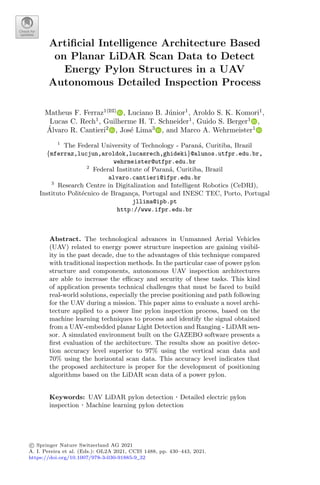

![LiDAR-Based Architecture for Autonomous UAV Pylon Inspection 433
controllers can work with these GNSS modules data to provide high accuracy
positions to the aircraft, allowing autonomous mission programming. This tech-
nique is one of the most common solutions to provide precise horizontal position-
ing to UAV but demands good operational conditions to work properly. Some
environment conditions, like the presence of obstacles, antenna shadowing, mag-
netic field interference, and cloudy weather conditions, may affect the system
accuracy significantly [19], justifying the development of complementary posi-
tioning solutions to integrate the UAV control system.
A common approach to propose UAV position and navigation data is using
computer vision algorithms that collect images based on regular or stereoscopic
cameras embedded on the UAV. Some review papers were published about this
subject, presenting the main applications and challenges about the practical use
of vision-based UAV control algorithms. This includes the influence of outdoor
light variation, difficult of identifying object clues in the images to provide data
information for the vision algorithms, and the high variability of the flight sites
composition and objects, making it hard to define a general image algorithm
processing for all kind of application [1,10,12].
Considering the specific area of energy power structure autonomous inspec-
tion, two kinds of computer vision algorithm approaches are found in the lit-
erature: (a) the power line following applications, used for a long-range and
long-distance visual inspection, and (b) the pylon detection and localization for
small distance detailed inspection operation.
The line following applications has the main objective of identifying the posi-
tion of the UAV related to the energy power cables and transmission structure
during its displacement along the lines when the aircraft capture images of the
energy cables and components for an overview of the structural conditions. In
this situation, the algorithm must keep the UAV navigation in the correct path
and distance from the structures during the aircraft displacement (10.0 m to
50.0 m commonly), using the images captured to provide information to the dis-
tance and orientation estimators, feeding the flight controller. Most proposals use
image processing techniques to extract the power line from an image and calcu-
late the position and orientation of the UAV related to it [2,6,9,11,13,14,18].
Another approach uses pylon detection and identification on images to pro-
vide a direction to the UAV displacement. In these cases, the vision algorithms
extract the pylon features from the image and calculate its position, feeding the
flight control hardware to pursuit the “target” and displace it to the next pylon.
An example of this approach is presented in the work [8].
Some works presented in the literature apply vision algorithms to provide
a high accuracy position data to the UAV related to the power pylon when
it executes the flight in small distances (2.0 m to 6.0 m commonly) to capture
detailed images of the structure components.
A pylon distance estimation algorithm based on monocular image processing
is presented in [3]. It uses the UAV displacement based on the GPS and the air-
craft’s IMU (Inertial Measurement Unity) data to calculate the pylon position
using the image match points for two consecutive images. A position measure-](https://image.slidesharecdn.com/optimizationlearningalgorithmsandapplications-231204021346-9e8015c0/85/Optimization-Learning-Algorithms-and-Applications-pdf-441-320.jpg)
![434 M. F. Ferraz et al.
ment error lower than 1.0 m has been reported as a result (for the best samples)
of a 10.0 m distance flight in real-world experiments, using a pylon model.
Another similar work proposes a “Point-Line-Based SLAM” technique based
on a monocular camera to calculate the center of the pylon. A 3D point cloud is
estimated from the monocular images at each algorithm interaction, providing
the capability to calculate the distance from the UAV and the pylon. The results
present an average position error of 0.72 m [5].
Using LiDAR sensors to provide distance data for energy power inspection
is a good approach to solve problems related to the inspection tasks. The main
application of this kind of sensor in UAV energy power inspection is focused on
the mapping of the structures using the LiDAR point cloud data to reconstruct
the real conditions of the transmission lines [4,9,16,17].
Another approach that proposes a distance estimation of a pylon for a
detailed inspection application, based on a planar LiDAR sensor, is presented.
In the work, a planar LiDAR carried onboard by a multi-rotor aircraft collects
horizontal data from the pylon structure and uses such information to calcu-
late the geometric centroid of the pylon. One issue of this technique is that it
demands the aircraft to keep the alignment to the pylon to obtain proper data
to feed the position calculation. Also, the inclination of the measurement plane,
due to the movement of the aircraft, has a significant influence on the position
error calculated by the algorithm, as described in [15].
This brief state-of-art review shows that intelligent computing algorithms
based on a planar LiDAR sensor data can provide a significant contribution to
this specific area of application, especially when they are employed to identify
the pylon position/orientation and to calculate its distance from a UAV flying
close to it. The work described in the present paper is a first evaluation of the
application of machine learning algorithms to face the mentioned challenges.
3 Problem Description
The power pylon detailed inspection demands the UAV displacement around its
structure. In this operation, the technician goal is to achieve a close-up image of
the pylon components to verify their integrity. This operation requires that the
aircraft stays hovering close to the targets points, typically within 4.0 m. The
robustness of the flight control depends on the correct evaluation of the UAV
position, in this case, with high accuracy. Although a centimeter-level accuracy
obtained by a DGNSS system is suitable for this operation, the malfunction of
this system demands the proposal of additional positioning systems to assure
the security of the flight, as explained earlier.
This work main goal is, as described below, to run an initial evaluation of a
positioning architecture based on an Artificial Intelligence algorithm to detect
an electric power pylon close to a UAV in short distances, in order to assist
the detailed pylon inspection tasks. Such an architecture is based on two planar
LiDAR sensors to scan, respectively, the horizontal and vertical planes. Each](https://image.slidesharecdn.com/optimizationlearningalgorithmsandapplications-231204021346-9e8015c0/85/Optimization-Learning-Algorithms-and-Applications-pdf-442-320.jpg)
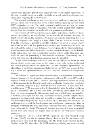
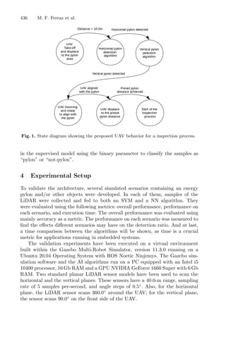
![LiDAR-Based Architecture for Autonomous UAV Pylon Inspection 437
Eight distinct scenarios were built to allow the data collection for the training
and evaluation of the horizontal AI algorithms, as shown in Fig. 2.
Fig. 2. Images of the experiment scenarios. a) Only a pylon in the field. b) Several
buildings and one pylon. c) Several trees and one pylon in the field. d) A complex
building structure, a water tank and one pylon. e) Several buildings, one pylon and
one tree. f) Several buildings; no pylon. g) Several trees in the field close from each
other; no pylon. h) A complex building structure, a water tank; no pylon.
A 3D STL pylon model from GRABCAD [7] website was imported to the
GAZEBO. To execute the data collection for the horizontal LiDAR, the sensor
was randomly displaced around the pylon on a range from 2.0 m to 10.0 m in dif-
ferent heights between 2.0 m and 20.0 m. The pylon height was set to 30.0 m. For
all the experiments a practical approach was considered in the sensor horizontal
stabilization. It was defined that the LiDAR sensor was attached to a stabilized
gimbal that keeps the sensor always scanning in a horizontal or vertical plane.
A random horizontal alignment noise with 1.0-degree range was added to the
sensor position to simulate the stabilization error present on the gimbal mecha-
nism. Figure 3 shows an example of the horizontal point map LiDAR detection
on a simulation in a complex environment.
For each position, the sensor captures a 360-degree planar point data and
store it into a vector. All samples for each scenario were stored and pos-processed,
indicating the presence or not presence of the pylon in the scenario. The training
set was composed of 80% of the collected samples and the test set was composed
of 20% of the collected samples.
Table 1 presents the results of the SVM algorithm versus the NN algorithm
for the horizontal LiDAR data experiment.
For the vertical data collection, the LiDAR sensor was configured in the same
conditions as the horizontal sensor, however, it scans a 90.0-degree range. A total
of 17500 samples have been captured and used as the training and test data. The
main difference for this data collection is that the sensor was keep pointed to the
pylon in the scenario with a pylon present to assure that the collected samples
contain the detection of the pylon segment. These samples have been tagged as
“pylon” to feed the training set. In the other scenarios, the sensor was randomly
placed in the space inside a 10.0-m radius from the center of the scene, and also](https://image.slidesharecdn.com/optimizationlearningalgorithmsandapplications-231204021346-9e8015c0/85/Optimization-Learning-Algorithms-and-Applications-pdf-445-320.jpg)
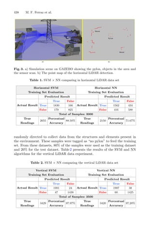
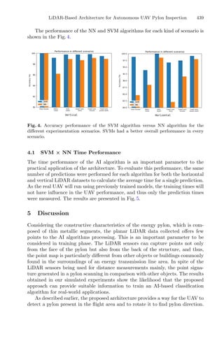
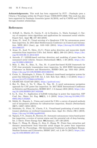
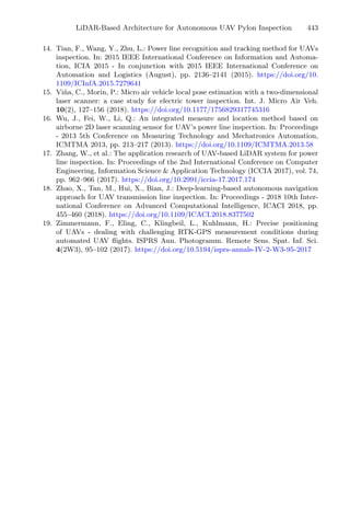

![Machine Vision to Empower an Intelligent
Personal Assistant for Assembly Tasks
Matheus Talacio1,2
, Gustavo Funchal1(B)
, Victória Melo1
, Luis Piardi1,2
,
Marcos Vallim2
, and Paulo Leitao1
1
Research Center in Digitalization and Intelligent Robotics (CeDRI),
Instituto Politécnico de Bragança, Campus de Santa Apolónia,
5300-253 Bragança, Portugal
{gustavofunchal,victoria,piardi,pleitao}@ipb.pt
2
Universidade Tecnológica Federal do Paraná (UTFPR),
Avenida 7 de Setembro 3165, Curitiba 80230-901, Paraná, Brazil
matheustalacio@alunos.utfpr.edu.br, mvallim@utfpr.edu.br
Abstract. In the context of the fourth industrial revolution, the inte-
gration of human operators in emergent cyber-physical systems assumes
a crucial relevance. In this context, humans and machines can not be
considered in an isolated manner but instead regarded as a collabora-
tive and symbiotic team. Methodologies based on the use of intelligent
assistants that guide human operators during the execution of their oper-
ations, taking advantage of user friendly interfaces, artificial intelligence
(AI) and virtual reality (VR) technologies, become an interesting app-
roach to industrial systems. This is particularly helpful in the execution
of customised and/or complex assembly and maintenance operations.
This paper presents the development of an intelligent personal assis-
tant that empowers operators to perform faster and more cost-effectively
their assembly operations. The developed approach considers ICT tech-
nologies, and particularly machine vision and image processing, to guide
operators during the execution of their tasks, and particularly to verify
the correctness of performed operations, contributing to increase produc-
tivity and efficiency, mainly in the assembly of complex products.
1 Introduction
The 4th industrial revolution is pushing the adoption of emergent technologies,
e.g., Internet of Things (IoT), Artificial Intelligence (AI), Big data, collaborative
robots and Virtual Reality (VR), aiming to transform the way factories operate
to increase their responsiveness and reconfigurability. In particular, Industry 4.0
enables the increasing level of automation and digitization in the factories of the
future [5], with Cyber-Physical Systems (CPS) acting as a backbone to develop
such emergent production systems and contributing to develop smart processes,
machines and products. CPS aims to connect the various physical components,
e.g., sensors and actuators, with cyber systems composed by controllers and
communication networks to achieve a common goal [9].
c
Springer Nature Switzerland AG 2021
A. I. Pereira et al. (Eds.): OL2A 2021, CCIS 1488, pp. 447–462, 2021.
https://doi.org/10.1007/978-3-030-91885-9_33](https://image.slidesharecdn.com/optimizationlearningalgorithmsandapplications-231204021346-9e8015c0/85/Optimization-Learning-Algorithms-and-Applications-pdf-453-320.jpg)
![448 M. Talacio et al.
In this emergent CPS environment, humans have a very important role
since they are the most flexible elements in automated systems, being required
their symbiotic integration. In particular, instead of performing repetitive and
monotonous tasks that can be fully automated, humans will be requested to
perform add-value tasks, e.g., assembly of complex and/or customized products
or performing maintenance interventions.
In this context, intelligent assistants and virtual interfaces can be used to
assist humans to realize their manual operations in a faster and more cost-
effective manner, taking advantage of the huge amount of data available at the
shop floor, as well as the emergent ICT technologies, e.g., AI and VR [3]. These
intelligent assistants can support the online monitoring of the equipment con-
dition during the execution of the assembly and maintenance operations, and
combine this information with diagnostic reports and their previous experience
in analogous situations, to determine the best action plans to be carried out. In
such systems, besides the intelligence behind the guidance system, it is important
to consider automatic systems that dynamically verifies the correctness of per-
formed operations, warning the need to correct the operation and only allowing
to proceed in case the operation is complete and successfully performed.
Such automatic verification usually involves the use of machine vision tech-
niques, which in industry context presents several constraints, namely related
to environmental illumination and shadowing, time response and the irregular
geometries of the pieces to be checked. These systems can be empowered with
the use of AI techniques and should be integrated with the other functionalities
of the intelligent assistants.
Having this in mind, this paper describes the development of a machine vision
solution, as part of an intelligent personal assistant (IPA), that supports human
operators to perform faster and more cost-effectively their assembly operations.
In particular, the IPA application uses ICT technologies and image processing
techniques to guide operators to assembly correctly customized and complex
products, checking the correctness of the performed operations. The activities
carried out by the operator are supervised through an intelligent system that
will verify the assertiveness of the assembly to ensure that the operation cycle
will only end when the system detects that the assembly is correct, even for the
scenarios considering 3D assemblies, in which the final product is assembled step
by step, and each step is understood as a complete activity. Since the algorithm
is executed in real-time, a check to verify if an operator is modifying the assembly
is included. The developed solution allows to increase the productivity of oper-
ators through the direct integration with emerging technologies, and strongly
contributes for the human integration with highly automated applications.
The rest of the paper is organized as follows. Section 2 contextualizes the
related work on developing intelligent assistants, as well as the use of machine
vision to verify the correctness of assembly operations. Section 3 presents the IPA
system architecture for the case study and Sect. 4 describes the development of
the machine vision system to verify the correctness of assembly operations for
the two scenarios considered in the case study. Section 5 discusses the achieved](https://image.slidesharecdn.com/optimizationlearningalgorithmsandapplications-231204021346-9e8015c0/85/Optimization-Learning-Algorithms-and-Applications-pdf-454-320.jpg)
![Machine Vision to Empower an Intelligent Personal Assistant 449
experimental results, and particularly the user experience. Finally, Sect. 6 rounds
up the paper with the conclusions and points out the future work.
2 Related Work
Industry 4.0 relies on the use of CPS complemented with emergent digital tech-
nologies to achieve more intelligent, adaptive and reconfigurable production sys-
tems. Also important is the integration of the human operators into the produc-
tion processes for enhanced product value, achieving manufacturing flexibility in
complex human-machine systems, where humans and machines can not be con-
sidered in an isolated manner but instead regarded as a collaborative team [8].
This requires the presence of operators on the design of human-centred adaptive
manufacturing systems, allowing a symbiotic integration.
However, the execution of some operations, e.g., assembly and maintenance,
is normally complex and requires high-level expertise from the operators to exe-
cute them efficiently in short time, with the required quality and with the mini-
mal impact on the normal production cycles. This requires to enable the human-
machine collaboration, through the use of innovative technologies, e.g., machine
vision, machine learning and VR, that will support the operators during the
realization of their tasks.
In this context, IPA is a guidance software system that can support the
execution of operations, facilitating the interaction between the operators and
machines or computers, based on data mining from images, video, and voice
commands captured from sensors distributed in the environment [6,14]. The use
of IPA, as an intelligent assistant to inform the operator with real-time and his-
torical data and guide through the best action plan to perform the operation [7],
can improve the quality of executed operations, particularly in case of complex
and/or customised ones. As an example, maintenance technicians can use an
IPA system to obtain useful real-time information about the machine condition,
recommendations and actions to be taken, as well as useful information, e.g.,
documents, websites or videos [4]. These systems can provide real-time informa-
tion and instructions, replacing traditional methods that rely on printed manuals
and real machines that can be damaged [13].
The more common commercial versions of IPA are, e.g., Amazon Alexa,
Microsoft Cortana, Google Assistant or Apple Siri. In industrial environments,
IPA are, e.g., being used to training as a means of learning through the first-
person experience [1,10], to train operators in new machine maintenance pro-
cedures [16] and to support operators in performing complex and customised
assembly tasks and maintenance operations [15].
The use of IPA can include mechanisms to automatically verify the correct-
ness of the performed operations, namely assembly operations. In this context,
artificial vision, also known as machine vision, plays an important role in the
supervision of assembly operations since it allows the acquisition and analy-
sis of image data, which would not be possible only by inference of context in
software. In industrial environments, the verification of 3D product assemblies](https://image.slidesharecdn.com/optimizationlearningalgorithmsandapplications-231204021346-9e8015c0/85/Optimization-Learning-Algorithms-and-Applications-pdf-455-320.jpg)
![450 M. Talacio et al.
is not possible by using simple 2D images, which requires to consider alterna-
tive cameras that allows to measure the distance of points in the field of view,
providing a 3D image of the scene. Several technologies can be considered to
accomplish this objective, e.g., TOF (Time of Flight), used by Microsoft Kinect
2.0 and Microsoft Azure Kinect, and stereo vision, used by Intel Realsense and
Stereolabs ZED. The acquired images are analysed by using image processing
techniques to recognize shapes and objects, e.g., contour matching, morpholog-
ical operations and feature detection. In case of recognition of complex shapes,
these techniques can be combined with machine learning algorithms.
The referred commercial intelligent assistants solutions usually provide
speech recognition functionalities but miss the image recognition, which is crucial
in industrial environments. Additionally, the use of such intelligent assistants in
industrial environments is still rare, with the majority running as laboratory pro-
totypes, mainly due to the industrial constraints and complexity, e.g., lighting,
objects geometry and object overlay.
Several aspects can influence the use and confidence of the IPA technology,
e.g., usability, security and privacy [2]. At the practical level, there are some
challenges to be faced regarding the adoption of IPA supporting technologies in
industrial environments. These solutions need to be matured to avoid creating
entropy within the maintenance process and operators need to be adequately
trained to operate the system in a proper manner. The IPA’s human-interaction
barrier models need to be improved, and AI systems need to prove reliabil-
ity. Another aspect is related to the ergonomic evolution of the head mounted
devices, which need to be more comfortable for operators to use during the entire
shift or even complete the maintenance intervention [12].
3 System Architecture for the Intelligent Personal
Assistant
This section presents the setup of the assembly workbench and the system archi-
tecture of the IPA that will be mentoring operators to the execute assembly
operations based on LEGO pieces from different shapes and colours.
3.1 Description of the Case Study
In this work, an IPA is used to support operators to perform their customised
and/or complex assembly operations in a more efficient manner. For this pur-
pose, the IPA is combined with a workbench structure, illustrated in Fig. 1,
providing an intuitive and guidance information to the user regarding the task
to be performed, as well as the capability to verify the correctness of the opera-
tion execution. As example, the IPA informs the operator about the action plan
to perform the operation, namely which step to be executed, how to execute the
step, and which piece or tool should be used in this step.
The physical structure comprises several devices that support the human-
machine interface. In terms of data collection, the workbench has an Intel](https://image.slidesharecdn.com/optimizationlearningalgorithmsandapplications-231204021346-9e8015c0/85/Optimization-Learning-Algorithms-and-Applications-pdf-456-320.jpg)
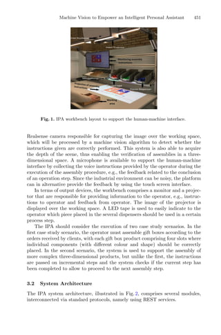
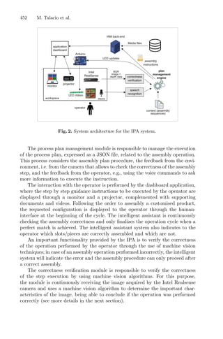

![454 M. Talacio et al.
All colours
of the object
analysed?
Yes
No
Image acquisition
(RGB colorspace)
Conversion to the
HSV colorspace
Colour identification
filter (Thresholding
operations)
Add to list with
properties of found
objects
Returns list with
properties of all objects
found in the image
Find contours
Fig. 3. Algorithm for the image recognition.
human eyes [11]. Considering the image after the colour space conversion, the
use of the OpenCV library, and particularly the inRange function, allows apply-
ing a threshold filter to isolate the pixels from the image by defining a range
in the colour space. As result, a binary image is obtained, with the pixels that
are within the defined range for each colour assuming the white colour and the
pixels that are not within the range assuming the black colour. This process is
performed for all the available colours of objects to be identified and the range
is defined for each colour. From the binary image it is possible to find the con-
tour of the different objects by using the findContours method, which extracts
information about the area, center of mass and vertex position of the object.
This image recognition algorithm is performed for both case study scenarios.
However, the algorithm to verify the assembly correctness is dependent of the
scenario and will be described in the following sections.
4.2 Verification Algorithm for the Gift-Box Assembly
In this scenario, the application generates a configuration for the gift-box accord-
ing to the received orders, i.e. which pieces (defined in terms of shape and colour)
should be placed in each one of the four box slots. The operator receives the
information related to this configuration, through the projector and monitor,
and performs the assembly operation by placing the pieces in the target slots
of the gift-box. The requirements to confirm the correct assembly include the
verification if only one piece is placed in each slot and if the piece has the colour
as requested in the configuration instructions. The algorithm to verify the cor-
rectness for the gift-box assembly is illustrated in Fig. 4.
The image recognition algorithm described in the previous section is used to
list the objects present at the scene. Then, for the gift-box assembly verification
algorithm, the pointPolygonTest function from the OpenCV library, is used to](https://image.slidesharecdn.com/optimizationlearningalgorithmsandapplications-231204021346-9e8015c0/85/Optimization-Learning-Algorithms-and-Applications-pdf-460-320.jpg)
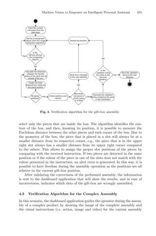
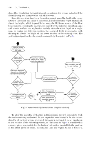
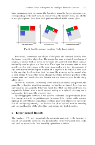
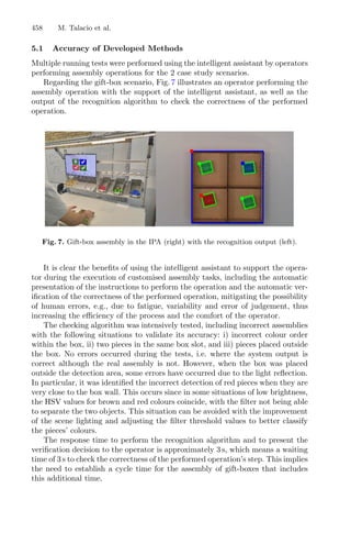
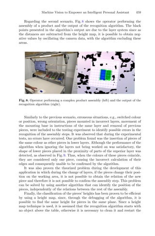
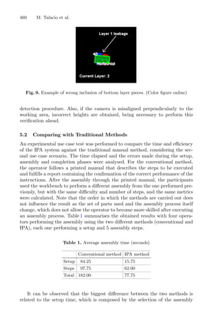

![Smart River Platform - River Quality
Monitoring and Environmental Awareness
Kenedy P. Cabanga1,2
, Edmilson V. Soares1,2
, Lucas C. Viveiros1
,
Estefânia Gonçalves2
, Ivone Fachada2
, José Lima1
,
and Ana I. Pereira1(B)
1
Research Centre in Digitalization and Intelligent Robotics CeDRI,
Instituto Politécnico de Bragança, 5300-252 Bragança, Portugal
{a36074,a39189}@alunos.ipb.pt, {viveiros,jllima,apereira}@ipb.pt
2
Centro de Ciência Viva de Bragança, Bragança, Portugal
{egoncalves,ifachada}@braganca.cienciaviva.pt
Abstract. In the technology communication era, the use of the Inter-
net of Things (IoT) has become popular among other digital solutions,
since it offers the integration of information from several organisms and
at several sources. By means of this, we can access data from distant
locations and at any time. In the specific case of water monitoring, the
conventional outdated measurement methods can lead to low efficiency
and complexity issues. Hence, Smart systems rise as a solution for a
broad of cases. Smart River is a smart system platform developed to
optimize the resources and monitoring the quality of water parameters
of the Fervença river. The central solution is based at Centro Ciência
Viva de Bragança (CCVB), one of the 21 science centers in Portugal
that aims to promote the preservation and environmental awareness for
the population. By using the IoT technologies, the system allows real-
time data collection with low cost and low energy consumption, being
a complement of existing projects that are being developed to promote
the ecological importance of natural resources. This paper covers sensor
module selection for data collection inside the river and data storage.
The parameters of the river are visualized using a program developed in
Unity engine to present data averages and comparison between weeks,
months, and years.
Keywords: Smart systems · Internet of Things (IoT) · Water
parameters
1 Introduction
Nowadays, the fourth industrial revolution is becoming increasingly popular
among researchers and employees because of its broad contributions in different
sectors. Among its different areas (virtual and augmented reality, artificial intel-
ligence, advanced robots, autonomous vehicles, cloud computing, big data and
block-chain between others) [1,2] the Internet of Things (IoT) is standing out
and growing rapidly.
c
Springer Nature Switzerland AG 2021
A. I. Pereira et al. (Eds.): OL2A 2021, CCIS 1488, pp. 463–474, 2021.
https://doi.org/10.1007/978-3-030-91885-9_34](https://image.slidesharecdn.com/optimizationlearningalgorithmsandapplications-231204021346-9e8015c0/85/Optimization-Learning-Algorithms-and-Applications-pdf-469-320.jpg)
![464 K. P. Cabanga et al.
Overall, the main advantage of IoT technology is the connections since it
allows the communication between many devices to share information inside
a cloud-based data system. Many points can be connected in any place, any
distance, and any time through the internet. This enables a better efficiency for
fast information delivery with low-cost and effort on building intelligent solutions
using software, sensors, vehicles, and electronic devices interconnected [2].
Whereas the conventional methods of water quality monitoring need to dis-
locate to the place to monitor the water directly or by analyzing it in the labo-
ratory. The proposed system takes advantage of the trend technologies of IoT to
build a smart solution. Smart River platform is a set of intelligent and intercon-
nected systems through the cloud to measure the water parameters and quality
of the Fervença river in Bragança, Portugal [5].
Fervença River is a border affluent of Sabor river, has its spring located in the
Fontes Barrosas village and crosses the city of Bragança, being one of the main
hydric resources for farming activities in the small communities of the region. It
is also an extensive source of biodiversity in its waters and the riverside, inside
and outside of the city’s territory.
The rivers and streams are a priceless resource, but pollution from urban and
agricultural areas pose a threat to the water quality. To understand the value
of water quality, and to effectively manage and protect the water resources, it’s
critical to know the current status of water-quality conditions, and how and why
those conditions have been changing over time.
The system aims to collect physical and chemical parameters from the Fer-
vença river, store all the data inside a cloud-based server, and display it in a
touchscreen monitor in one of the exhibits of the science center of Centro de
Ciência Viva de Bragança (CCVB). The exhibit aims to offer an interactive,
scientific and educational experience regarding the importance of carrying out
environmental monitoring combined with the latest communication technologies.
Besides, to improve the environmental awareness of CCVB visitors.
Currently, there is a great need for the use of decentralized and automated
systems for data collection in environmental systems. The data can be used for
the development of the technique that allows the improvement of environmen-
tal conditions, consequently, by improving the quality of people’s life who use
natural resources, as well as promoting sustainability.
Systems such as Smart River have been increasingly used in Smart Cities,
by allowing integration with other technologies and development of solutions
with shared databases. Combined with science communication techniques, the
module presents a tool that contributes to the population’s awareness on the
environmental value of the water.
This paper is organized as follows. Section 2 presents the literature review
associated with the sensor modules configuration, the network communica-
tion, Internet of Things (IoT) and LoRaWAN protocols. Section 3 addresses
the system architecture where the hardware and the communication scheme
is explained. Section 4 details the Smart River system development and the
management of the sensors installed at Bragança region. The water monitor-
ing through Node-Red and Unity applications is described at Sect. 5. Finally,
Sect. 6 presents some conclusions and points for future works.](https://image.slidesharecdn.com/optimizationlearningalgorithmsandapplications-231204021346-9e8015c0/85/Optimization-Learning-Algorithms-and-Applications-pdf-470-320.jpg)
![Smart River Platform 465
2 Theoretical Background
River quality monitoring systems seek to ensure high precision and accuracy of
data, timely reports, data averages, easy access to data and integrity. The river
is an important source of water for all cities and one of the main threats to its
sustainability is pollution. The existing methods for monitoring water quality
rivers are manual monitoring and continuous monitoring. These methods are
expensive and less efficient. Therefore, an intelligent river monitoring system
was proposed [12,13].
A peculiar effect of the IoT applications is the intelligently data control, which
is the result of the platform known as The Things Network (TTN). Whereas the
LoRaWAN protocol is used for sending data, and each device is capable of com-
municating through LoRa technology, known as End Nodes. The communication
occurs with the Gateway from sending data measurements taken by the sensors
and relevant information by the developed application [4,6,7].
The Gateway is responsible for creating a connection between the devices and
the network server and by receiving data from the various End Nodes. Besides
interpreting, storing, and passing the data into the network server. The Gateway
is always connected through the Network Server via the TCP and IP protocols,
either by the wired or wireless network. From the point of view of the End Nodes,
the Gateway is just a messenger forwarded to the Network Server.
Overall, TTN is an open-server platform in which the application’s servers
are built that interpret and present the data to the user. This server is able to
format the data that will be sent to the device and respond, when programmed
to do so, based on the data collected, autonomously and without the constant
need for human observation [8,9].
2.1 End Nodes
The LoRaWAN End nodes usually have sensors to detect a change in the param-
eters (e.g. temperature, humidity, accelerometers, GPS), a LoRa transponder
(responsible for transmitting the signals over LoRaWAN radio), and optionally,
a micro-controller. Besides the End node is battery-powered and uses low energy
approach, it requires attention from outside programs for checking the battery
charge. Depending on the system interface developed, it can show how last the
percentage of the battery. Some LoRa embedded sensors can run batteries to
last for a maximum of 5 years and transmit signals over distances to 10 km from
the other device connected through the network [3].
2.2 Gateways
One advantage of LoRaWAN technology is the worldwide connection between
gateways by the community of TTN. These devices support the operation of the
sensors to transmit the data to the LoRa Gateways. The package communication
process occurs by using the LoRa gateways which are responsible for using the
network with standard internet protocols (IP) to transmit data and to receive
data from the embedded sensors to the server [3].](https://image.slidesharecdn.com/optimizationlearningalgorithmsandapplications-231204021346-9e8015c0/85/Optimization-Learning-Algorithms-and-Applications-pdf-471-320.jpg)

![Smart River Platform 467
Table 1. Smart system components and specifications
Sensor
and components
Parameter
and function
Specifications
DHT11 Humidity and ambient
temperature
Voltage of 3 V to 5.5 V; electric current of
0.3 mA (measurement) 60 µA (standby);
temperature range from 0 ◦C to 50 ◦C;
humidity range: 20% to 90%; temperature
and humidity resolution is 16 bits; Accuracy
of ±1 ◦C and ±1% [14].
DS18B20 Water temperature Working Voltage of 3.2 V to 5.25 V DC;
Working Current of 2 mA (max); Resolution
of 9 to 12 bit programmable; Measuring
Range of −55 to 110 ◦C; Measurement
Accuracy of ±0.5 ◦C @ −10 to +80 ◦C; ±2
◦C @ −55 to +110 ◦C; output cables of
yellow (data), red (vcc), black (gnd); sensor
output interface of XH2.54-3P [15]
Analog pH pro V2 pH water level Supply voltage from 3.3 V to 5.5 V; Output
voltage of 0 V to 3.0 V; BNC probe
connector; PH2.0-3P signal connector;
PH2.0-3P signal connector; Measurement
accuracy of ±0.1 @ 25 ◦C; Dimension
42 mm * 32 mm/1.66 * 1.26 in; pH probe:
Probe type industrial grade; Detection range
of 0 to 14; Temperature range of 0 to 60 ◦C;
Accuracy of ±0.1pH (25◦); response time
1 min; probe life of 7 * 24 h 0.5 years
(depending on water quality) [16]
Electrical
conductivity
sensor V1
Water Conductivity Operating voltage +5.00 V; PCB size 45 ×
32 mm (1.77 × 1.26); Measuring range 1
ms/cm - 20 ms/cm; Operating temperature
5 - 40◦C; Accuracy ±10% F.S (using
Arduino 10 bits ADC); PH2.0 interface
(3-pin SMD); Conductivity electrode
(Constant Electrode K = 1, BNC
connector); Length of electrode cable about
60 cm (23.62); Standard conductivity
solution (1413 µs/cm and 12.88 ms/cm) x1
[17].
Transceiver
LoRa RFM95
Communication with
TTN
LoRa technology is available as Radio
Frequency communication on frequencies
433, 868 and 915 MHz. The operating ranges
of LoRa are part of the Industrial Scientific
and Medical (ISM) band, which different
intervals are reserved internationally for
ISM development
Atmega328p Microcontroller Memory; Timer/counter; A/D converter;
D/A converter; Parallel and Serial ports](https://image.slidesharecdn.com/optimizationlearningalgorithmsandapplications-231204021346-9e8015c0/85/Optimization-Learning-Algorithms-and-Applications-pdf-473-320.jpg)
![468 K. P. Cabanga et al.
3.2 Communication Network
Smart River systems communication occurs through the different IoT platforms
connected to the network. By using these platforms it is possible to collect
data through LoRaWAN technology and the Gateways. TTN aims to enable
low-power devices to use long-range Gateways and connect to a decentralized
open-source network. The final application allows exchanging data with high-
end precision and efficient connection. The Fig. 2 illustrates the sensor modules
registered on the platform [10].
Fig. 2. Devices
TTN uses the LoRaWAN protocol that defines the system architecture and
the communication parameters with LoRa technologies. These devices use low-
power LoRa networks, to connect to the Gateway and thus, enabling a high-
bandwidth connection, such as Wi-Fi, Ethernet, and GSM. All Gateways that
reach a device will receive messages from other devices on the net and re-forward
the message to them in the TTN. Thus, the network will reduplicate the messages
and select the best gateway to forward the messages in the queue to the downlink.
The Fig. 3 presents the communication scheme for data collection.
Fig. 3. Communication scheme](https://image.slidesharecdn.com/optimizationlearningalgorithmsandapplications-231204021346-9e8015c0/85/Optimization-Learning-Algorithms-and-Applications-pdf-474-320.jpg)
![470 K. P. Cabanga et al.
is possible to increase the network coverage area. In addition to installing Gate-
ways, anyone can install a Node and connect to a working Gateway at no cost
to use the network [11].
Today TTN has thousands of Gateways around the world and a very active
community using the platform, discussing and exchanging information. With the
use of the TTN network, applications that use IoT can be quickly prototyped,
moving from the validation phase to production with guaranteed scalability and
security [11].
After the data is collected by the sensors and communicated, all data is stored
in a cloud database that can be accessed through external applications. The
microcontroller is programmed to command the data collection by the sensors
and to send the information in byte format to the TTN server.
The microcontroller should use the “hibernate” mode for a defined interval
of 15 min and, if the battery is below 3 V, it goes into “hibernate forever”. By
this way, reducing energy consumption as much as possible and allowing a longer
battery life [11].
To allow access to data in an educational, scientific, and interactive way, two
user interface applications were developed: i) An application developed in Unity
engine, which is part of the permanent exhibition of Casa da Seda; ii) A Node.js
server application, which can be accessed via mobile phones linked. On example
is presented by Fig. 5.
The application made in Unity was developed in order to be educational and
intuitive, facilitating access to data averages and information about measured
parameters, collection points, and the application of LoRaWAN technology in
the development of the module.
Fig. 5. Parameters description](https://image.slidesharecdn.com/optimizationlearningalgorithmsandapplications-231204021346-9e8015c0/85/Optimization-Learning-Algorithms-and-Applications-pdf-476-320.jpg)
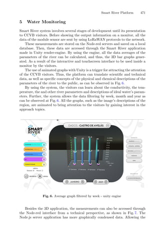


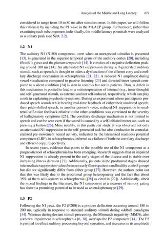

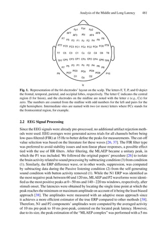
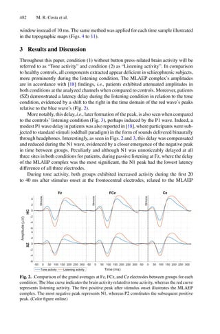
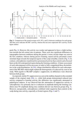
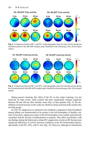


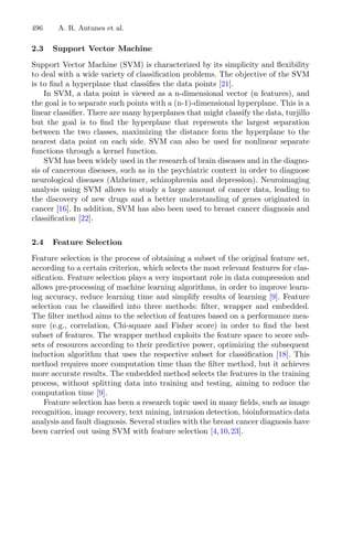
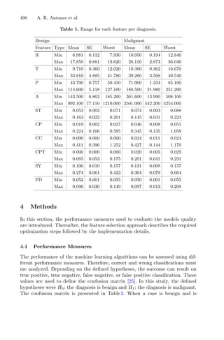
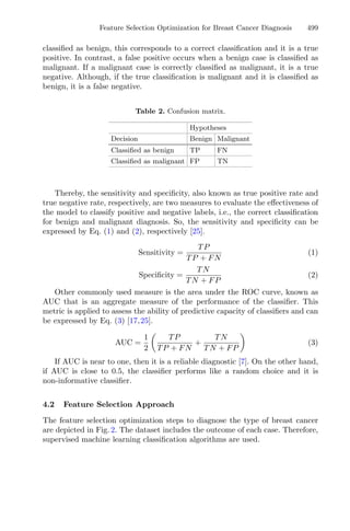
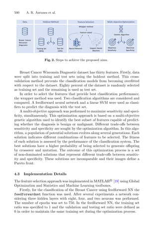
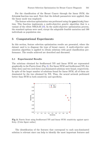
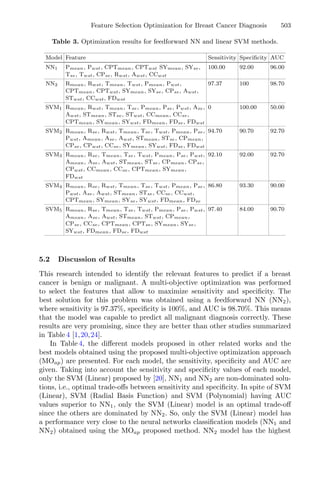
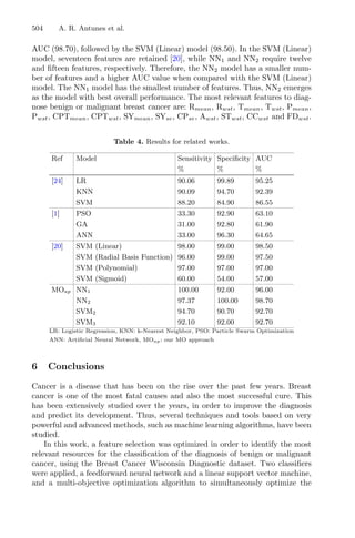


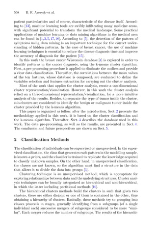

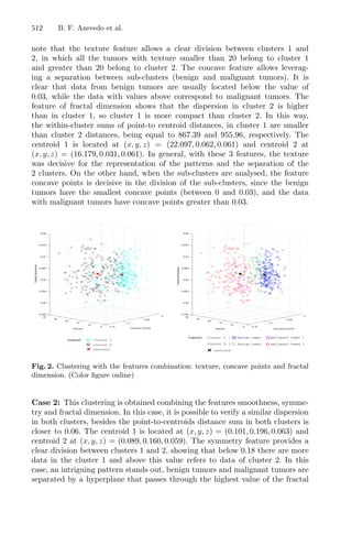
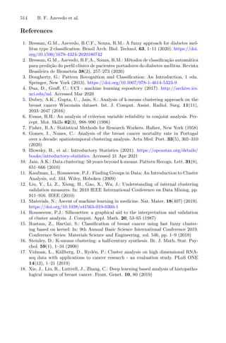


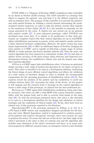
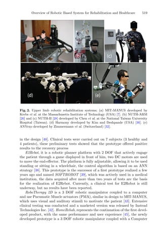
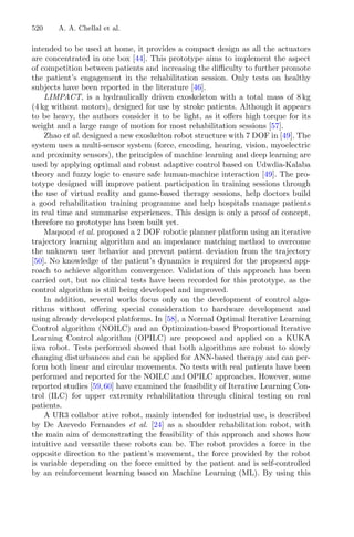
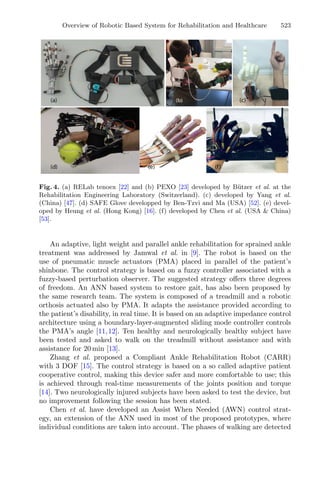

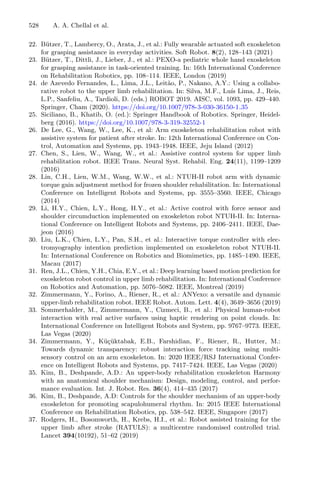


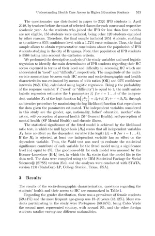
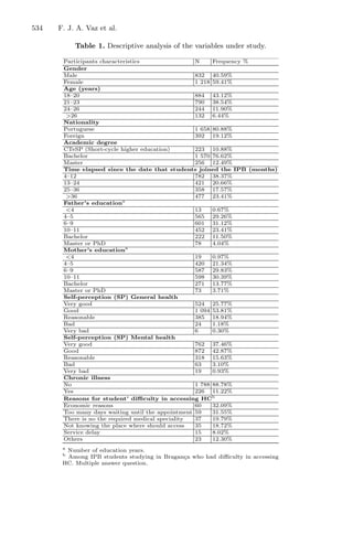

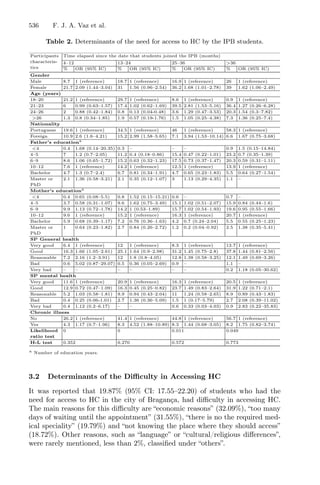


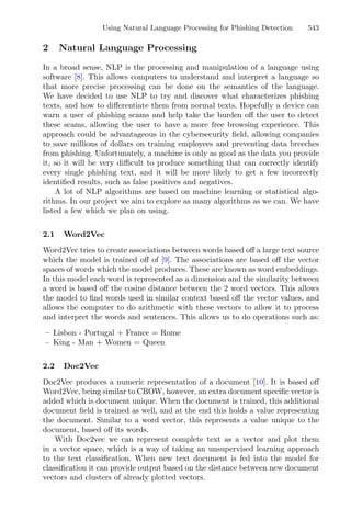

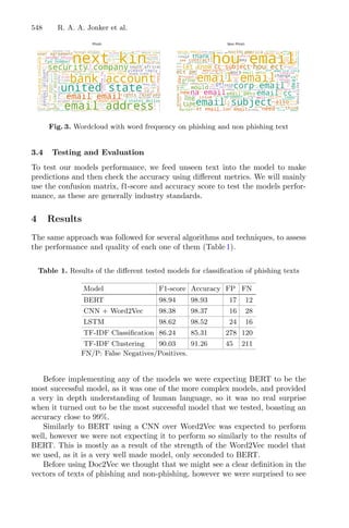
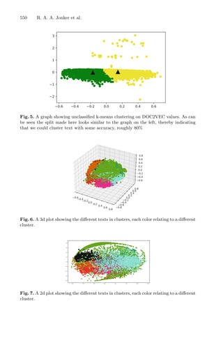
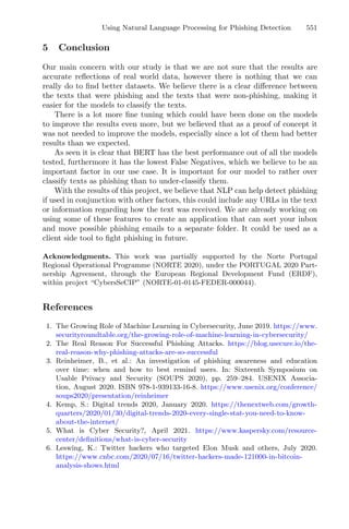


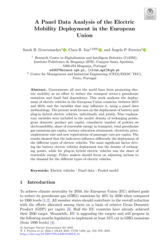
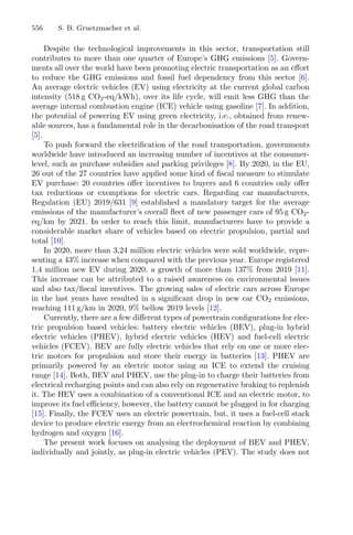
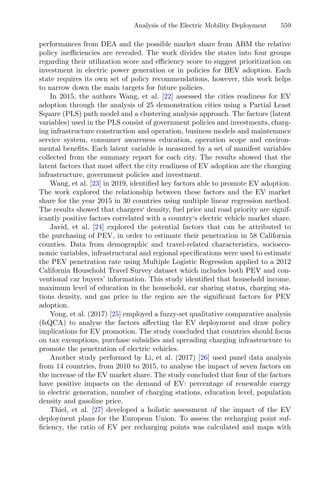
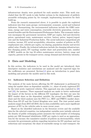
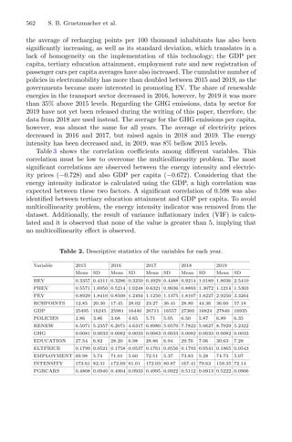
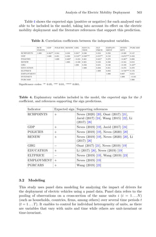
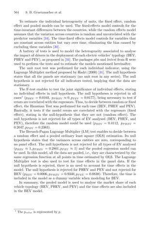
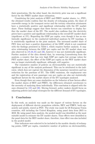


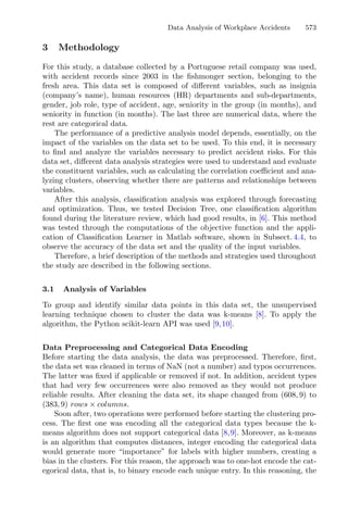
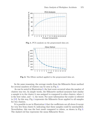
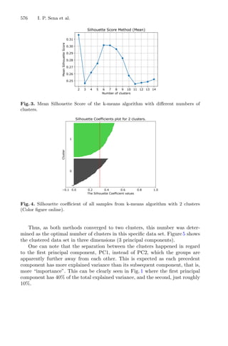
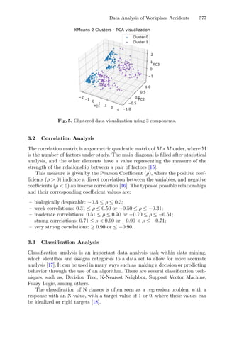
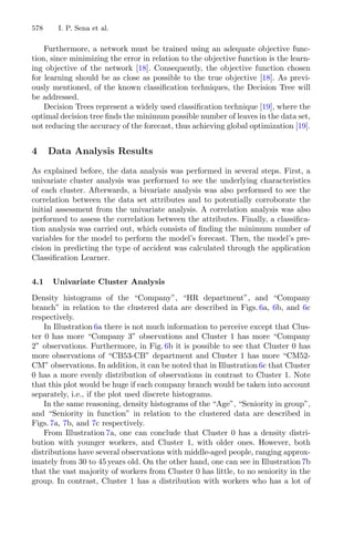
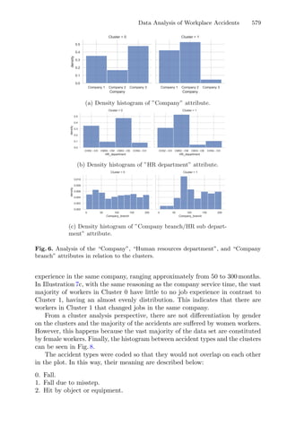
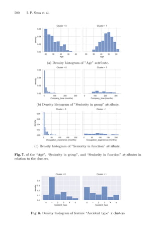
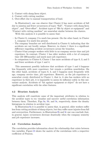
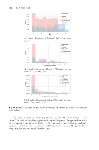
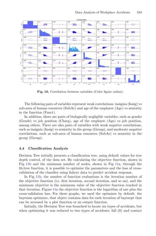
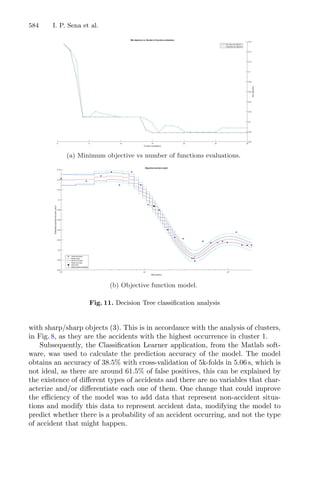

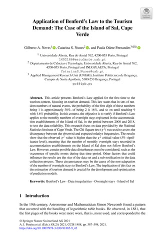


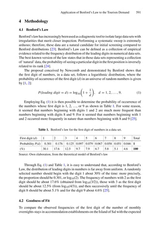
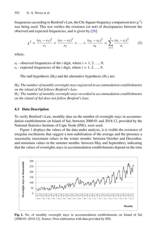
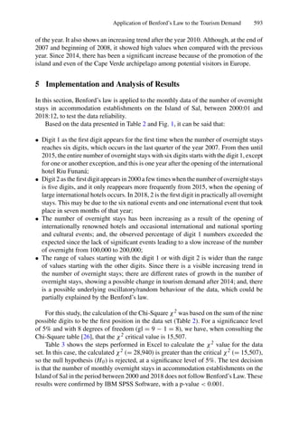
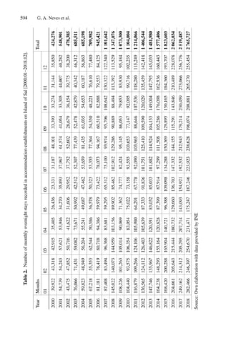
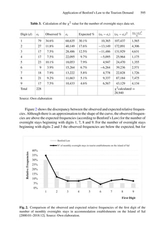


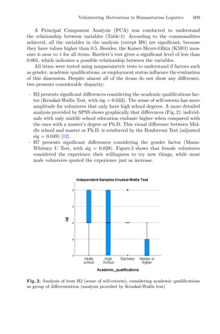
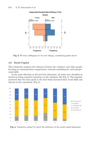
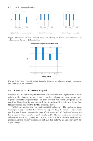
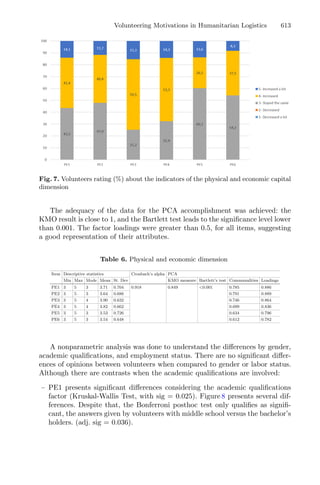
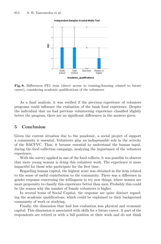

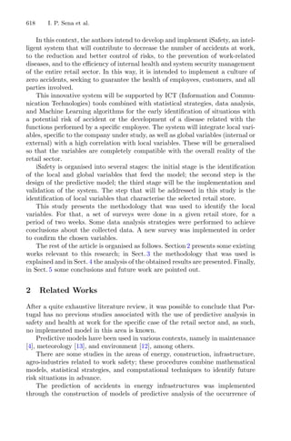


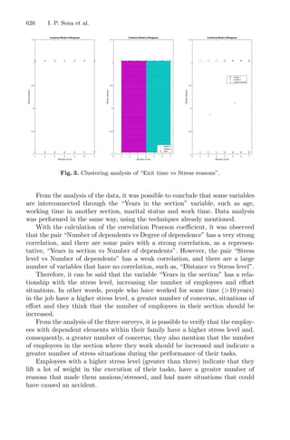


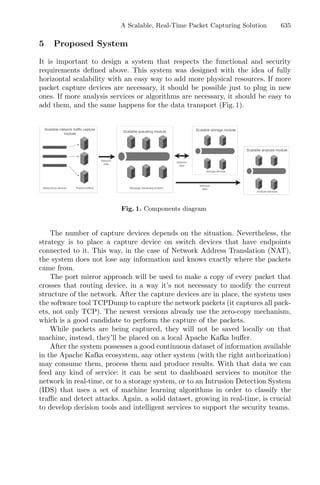


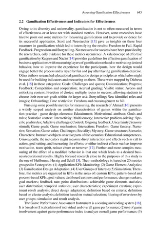
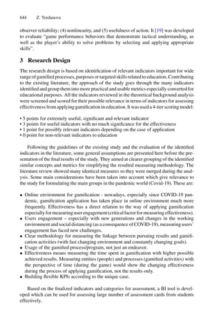
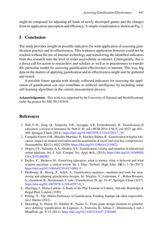


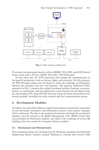


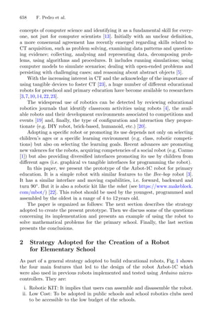
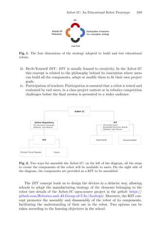


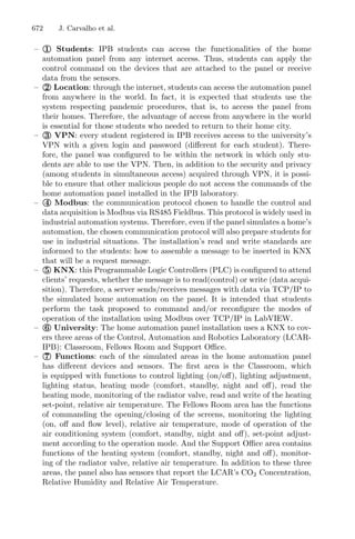
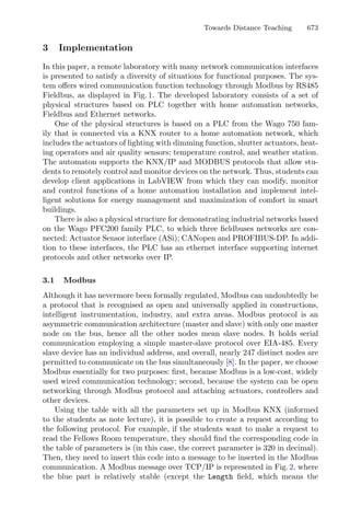

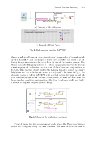


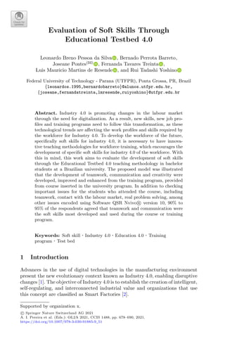


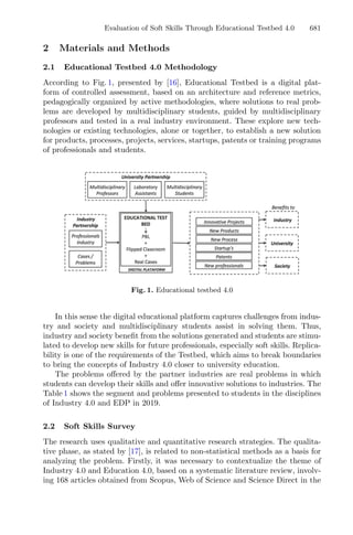
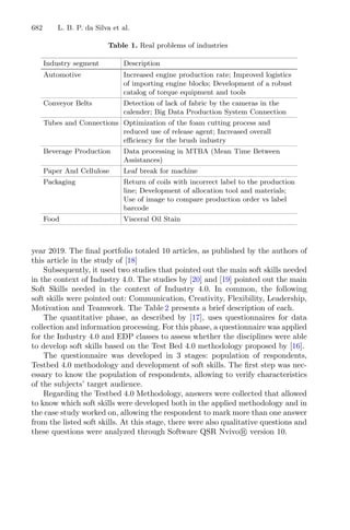


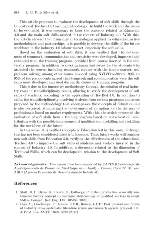
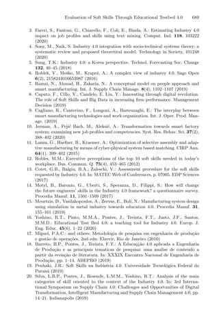


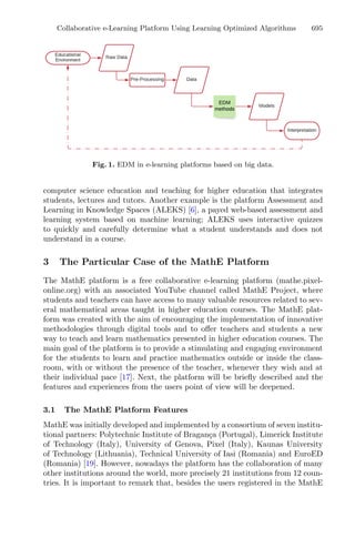


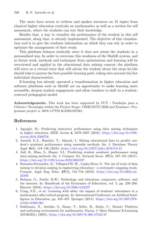


This document provides information about a conference titled "First International Conference, OL2A 2021" that was held from July 19-21, 2021 in Bragança, Portugal. It discusses the conference's organization, including its editors, scientific committee members, and topics. The conference focused on optimization, learning algorithms, and applications. It received 134 submissions and selected 52 accepted papers, including 39 full papers.


