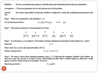
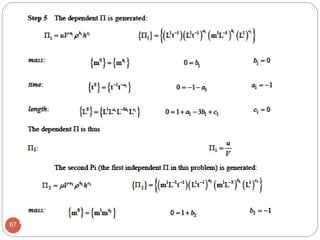
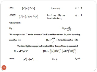
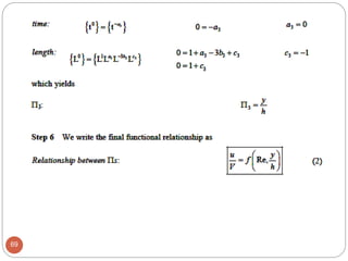
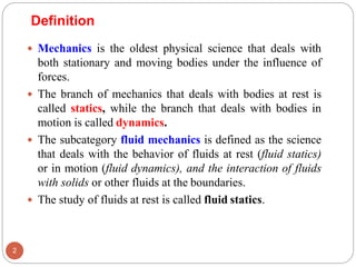
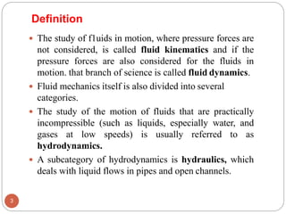
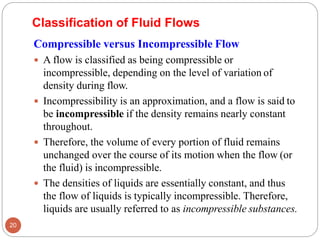
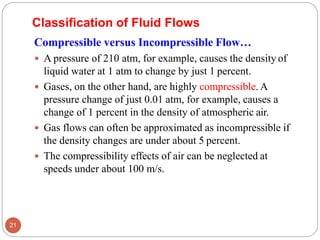
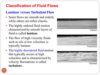
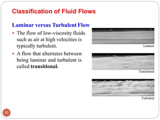
This document provides an introduction to fluid mechanics. It begins by defining mechanics, statics, dynamics, and fluid mechanics. Fluid mechanics deals with fluids at rest or in motion and their interaction with boundaries. The study of fluids at rest is called fluid statics, while considering pressure forces is called fluid dynamics. Fluid mechanics is divided into several categories including hydrodynamics, hydraulics, gas dynamics, and aerodynamics. The document then defines what constitutes a fluid and distinguishes between liquids and gases. It provides examples of applications of fluid mechanics in various engineering fields and classifies different types of fluid flows. Finally, it defines important fluid properties such as density, specific weight, specific volume, and viscosity.
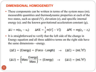
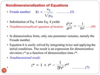
![Dimensions and Units…
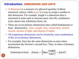
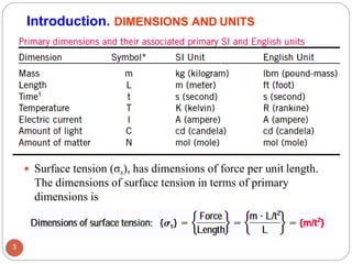
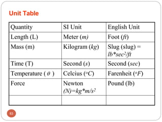
1 Newton – Force required to accelerate a 1 kg of mass
to 1 m/s2
1 slug – is the mass that accelerates at 1 ft/s2 when acted
upon by a force of 1 lb
To remember units of a Newton use F=ma (Newton’s 2nd
Law)
[F] = [m][a]= kg*m/s2 = N
To remember units of a slug also use F=ma => m = F / a
[m] = [F] / [a] = lb / (ft / sec2) = lb*sec2 / ft
84](https://image.slidesharecdn.com/ppt-fm-230922044820-a10b75a8/85/Ppt-FM-pdf-84-320.jpg)