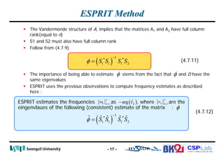
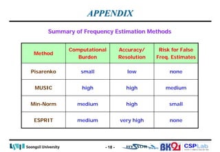
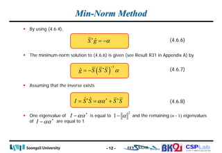
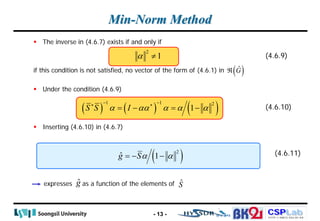
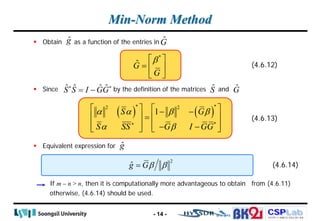
The document discusses various parametric methods for spectral estimation in communication signal processing, particularly focusing on Pisarenko and MUSIC methods, Min-Norm method, and ESPRIT. It outlines the procedural steps involved in each method for estimating frequency parameters, highlighting their computational efficiencies and accuracy levels. A summary table compares the computational burden, accuracy, resolution, and risks of false frequency estimates for each method.
![CSPLab
CSPLab
HTTP:/ / AMCS.SSU.AC.KR
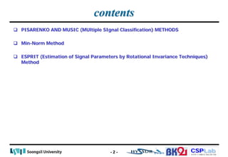
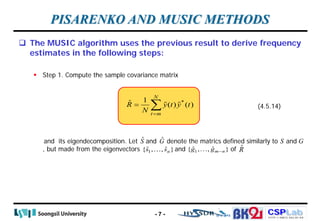
The Multiple Signal Classification (or Multiple Signal Characterization) [MUSIC] method and
Pisarenko’s method are derived from the covariance model (4.2.7) with m>n
Let
: eigenvalues of R
: orthonormal eigenvectors associated with
: orthonormal eigenvectors associated with
PISARENKO AND MUSIC METHODS
* 2
( )
R APA I m n
σ
= + >
1 2 m
λ λ λ
≥ ≥ ≥
1
{ , , }
n
s s
1
{ , , }
n
λ λ
1
{ , , }
m n
g g −
1
{ , , }
n m
λ λ
+
1 1
[ , , ] ( ), [ , , ] ( ( ))
n m n
S s s m n G g g m m n
−
× = × −
(4.5.4)
- 3 -
(4.2.7)](https://image.slidesharecdn.com/parametriclinespectra-241110095740-b04b9afe/85/Parametric_-Methods-for-line_spectra-in-pdf-3-320.jpg)
![CSPLab
CSPLab
HTTP:/ / AMCS.SSU.AC.KR
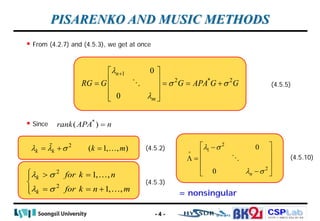
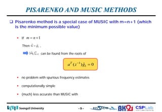
PISARENKO AND MUSIC METHODS
Spectral MUSIC:
Step 2a. Determine frequency estimates as the locations of the n highest peaks of the
function
* *
1
, [ , ]
ˆ ˆ
( ) ( )
a GG a
ω π π
ω ω
∈ − (4.5.15)
Root MUSIC:
Step 2b. Determine frequency estimates as the angular positions of the n (pairs of
reciprocal) roots of the equation
which are located nearest the unit circle
(4.5.16)
1 *
ˆ ˆ
( ) ( ) 0
T
a z GG a z
−
=
- 8 -](https://image.slidesharecdn.com/parametriclinespectra-241110095740-b04b9afe/85/Parametric_-Methods-for-line_spectra-in-pdf-8-320.jpg)
![CSPLab
CSPLab
HTTP:/ / AMCS.SSU.AC.KR
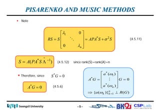
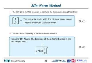
ESPRIT Method
Let
and
Where Im-1 is the identity matrix of dimension and
and are
It is verified that
where
D is unitary matrix
- 15 -
[ ] ( )
1 m 1
I 0 1
A A m n
−
= − × (4.7.1)
[ ] ( )
2 m 1
0 I 1
A A m n
−
= − × (4.7.2)
( ) ( )
1 1
m m
− × −
[ ]
m 1
I 0
− [ ]
m 1
0 I − ( )
1
m m
− ×
2 1
A A D
= (4.7.3)
1
0
0 n
i
i
e
D
e
ω
ω
−
−
=
(4.7.4)](https://image.slidesharecdn.com/parametriclinespectra-241110095740-b04b9afe/85/Parametric_-Methods-for-line_spectra-in-pdf-15-320.jpg)
![CSPLab
CSPLab
HTTP:/ / AMCS.SSU.AC.KR
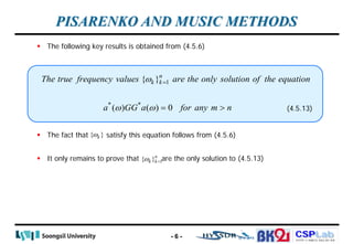
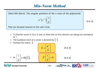
ESPRIT Method
Similarly to (4.7.1) and (4.7.2), define
From (4.5.12), we have that
where C is the nonsingular matrix given by
By using (4.7.1)-(4.7.3) and (4.7.7)
where
- 16 -
[ ]
1 m 1
I 0
S S
−
=
[ ]
2 m 1
0 I
S S
−
=
(4.7.5)
(4.7.6)
S AC
= (4.7.7)
n n
×
* 1
C PA S −
= Λ
1
2 2 1 1 1
S A C A DC S C DC S φ
−
= = = = (4.7.9)
1
C DC
φ −
(4.7.10)
(4.7.8)](https://image.slidesharecdn.com/parametriclinespectra-241110095740-b04b9afe/85/Parametric_-Methods-for-line_spectra-in-pdf-16-320.jpg)