Download to read offline
![PARAMETERIZED SURFACES AND SURFACE AREA
PORAMATE (TOM) PRANAYANUNTANA
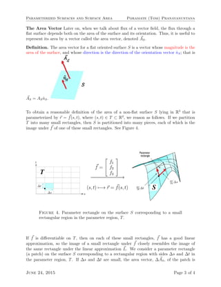
Definition. Given a function f : T ⊂
st-plane
R2
−→ S ⊂
xyz-space
R3
, we define the surface param-
eterized by r = f to be the set of points S =
r(s, t) ∈ R3
xyz-space
(s, t) ∈ T ⊂ R2
st-plane
.
f =
f1
f2
f3
−−−−−−−−−−−→
(s, t) −→ r = f(s, t)
Figure 1. The parameterization sends each point (s, t) in the parameter re-
gion, T, to a point (x, y, z) or position vector r = [f1(s, t), f2(s, t), f3(s, t)]T
on
the surface, S.
That is, S is the image of T under f. The equation r = f(s, t) is a parameterization of S.
We say that the parameterization by f =
f1
f2
f3
is smooth if the Jacobian matrix
Jf(s, t) =
f1s f1t
f2s f2t
f3s f3t
(1)
Date: June 24, 2015.](https://image.slidesharecdn.com/1098cb0f-1560-4e86-9ece-957f54588db1-150716230138-lva1-app6892/85/Parameterized-Surfaces-and-Surface-Area-1-320.jpg)
![PARAMETERIZED SURFACES AND SURFACE AREA
PORAMATE (TOM) PRANAYANUNTANA
Definition. Given a function f : T ⊂
st-plane
R2
−→ S ⊂
xyz-space
R3
, we define the surface param-
eterized by r = f to be the set of points S =
r(s, t) ∈ R3
xyz-space
(s, t) ∈ T ⊂ R2
st-plane
.
f =
f1
f2
f3
−−−−−−−−−−−→
(s, t) −→ r = f(s, t)
Figure 1. The parameterization sends each point (s, t) in the parameter re-
gion, T, to a point (x, y, z) or position vector r = [f1(s, t), f2(s, t), f3(s, t)]T
on
the surface, S.
That is, S is the image of T under f. The equation r = f(s, t) is a parameterization of S.
We say that the parameterization by f =
f1
f2
f3
is smooth if the Jacobian matrix
Jf(s, t) =
f1s f1t
f2s f2t
f3s f3t
(1)
Date: June 24, 2015.](https://image.slidesharecdn.com/1098cb0f-1560-4e86-9ece-957f54588db1-150716230138-lva1-app6892/75/Parameterized-Surfaces-and-Surface-Area-1-2048.jpg)
![Parameterized Surfaces and Surface Area Poramate (Tom) Pranayanuntana
Figure
2. The surface parameterized
by r = [s, 1 − t2
, t3
− t]T
, where
−1 ≤ s ≤ 1 and −1.2 ≤ t ≤ 1.2,
is not simple.
Figure 3. Astroidal sphere
parameterized by r =
[sin3
s cos3
t, sin3
s sin3
t, cos3
s]T
,
where 0 ≤ s ≤ π and
0 ≤ t < 2π, is not smooth.
has continuous entries and the normal vector nS = rs × rt = fs × ft never zero. A surface S
is simple if it has a parameterization that is given by a one-to-one function. A surface S is
said to be smooth if it has a one-to-one smooth parameterization.
The requirement that Jf(s, t) be continuous is to ensure a continuously varying normal nS to
the surface, and the nonvanishing cross product is to assure that the normal never becomes
the zero vector. These together hold the intuitive idea that a smooth surface is one without
cusps or creases. The definition of a simple surface is designed to take out self-intersections
such as that shown in Figure 2.
In Figure 3, for instance, is the surface parameterized by
r =
sin3
s cos3
t
sin3
s sin3
t
cos3
s
(2)
where 0 ≤ s ≤ π and 0 ≤ t < 2π. It is not smooth because, for example, nS = rs ×rt vanishes
when s = π/2 and t = 0; this is the sharp point on the surface at the point (1, 0, 0). A smooth
surface without self-intersections is sometimes called a manifold. Roughly speaking, a
manifold then should, in the vicinity of each point not on its boundary, resemble a plane.
Surface Area
Orientation of a Surface At each point on a smooth surface there are two unit normals,
one in each direction. Choosing an orientation means picking one of these normals at
every point of the surface in a continuous way. The unit normal vector in the direction of the
orientation is denoted by ˆnS. For a closed surface (that is, the boundary of a solid region),
we usually choose the outward orientation.
June 24, 2015 Page 2 of 4](https://image.slidesharecdn.com/1098cb0f-1560-4e86-9ece-957f54588db1-150716230138-lva1-app6892/85/Parameterized-Surfaces-and-Surface-Area-2-320.jpg)
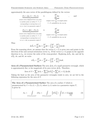

The document defines parameterized surfaces and discusses their surface area. A parameterized surface S is defined by a function f that maps points (s,t) in a parameter region T to points in R3. S has a smooth parameterization if the Jacobian of f is continuous and the normal vector is never zero. Surface area is approximated by dividing S into small parameter rectangles and taking the limit. The area of a parameterized surface S is given by the integral over the parameter region T of the cross product of the partial derivatives of the parameterization f with respect to s and t.