1. SURFACE INTEGRALS AND FLUX INTEGRALS
PORAMATE (TOM) PRANAYANUNTANA
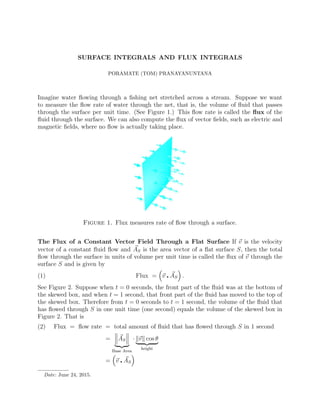
Imagine water flowing through a fishing net stretched across a stream. Suppose we want
to measure the flow rate of water through the net, that is, the volume of fluid that passes
through the surface per unit time. (See Figure 1.) This flow rate is called the flux of the
fluid through the surface. We can also compute the flux of vector fields, such as electric and
magnetic fields, where no flow is actually taking place.
Figure 1. Flux measures rate of flow through a surface.
The Flux of a Constant Vector Field Through a Flat Surface If v is the velocity
vector of a constant fluid flow and AS is the area vector of a flat surface S, then the total
flow through the surface in units of volume per unit time is called the flux of v through the
surface S and is given by
Flux = v AS .(1)
See Figure 2. Suppose when t = 0 seconds, the front part of the fluid was at the bottom of
the skewed box, and when t = 1 second, that front part of the fluid has moved to the top of
the skewed box. Therefore from t = 0 seconds to t = 1 second, the volume of the fluid that
has flowed through S in one unit time (one second) equals the volume of the skewed box in
Figure 2. That is
Flux = flow rate = total amount of fluid that has flowed through S in 1 second(2)
= AS
Base Area
· v cos θ
height
= v AS
Date: June 24, 2015.

2. Surface Integrals and Flux Integrals Poramate (Tom) Pranayanuntana
Figure 2. Flux of v through a flat surface with area vector AS is the volume
of this skewed box.
Figure 3. Surface S di-
vided into small, almost flat
pieces, showing a typical ori-
entation vector ˆn and area
vector ∆AS
Figure 4. Flux of a vector
field through a curved sur-
face S.
The Flux Integral To calculate the flux of a vector field F which is not necessarily con-
stant through a curved, oriented surface S, we divide the surface into a patchwork of small,
approximately flat pieces (like a wire-frame representation of the surface) as shown in Figure
3. Suppose a particular patch has area ∆AS. We pick an orientation vector ˆnS at a point on
the patch and define the area vector of the patch, ∆AS, as ∆AS = ˆnS∆AS. If the patches are
small enough, we can assume that F is approximately constant on each piece. (See Figure
4.) Then we know that
Flux through patch ≈ F ∆AS ,
so, adding the fluxes through all the small pieces, we have
Flux through whole surface ≈ F ∆AS .
As each patch becomes smaller and ∆AS → 0, the approximation gets better and we get
Flux through S = lim
∆AS →0
F ∆AS .
June 24, 2015 Page 2 of 4

3. Surface Integrals and Flux Integrals Poramate (Tom) Pranayanuntana
Thus, provided the limit exists, we define the following:
The flux integral of the vector field F through the oriented surface S is
S
F dAS = lim
∆AS →0
F ∆AS . (3)
If S is a closed surface oriented outward, we describe the flux through S as the flux
out of S, and it is denoted by
S
F dAS to emphasize that S is a closed surface.
Flux Integrals Over Parameterized Surfaces We now consider how to compute the
flux of a smooth vector field F through a smooth oriented surface, S, parameterized by
r = r(s, t) = f(s, t), for (s, t) in some region T of the parameter space. We write
S : r = r(s, t) = f(s, t), (s, t) ∈ T.
We consider a parameter rectangle on the surface S corresponding to a rectangular region
with sides ∆s and ∆t in the parameter region, T. (See Figure 5.)
Figure 5. Parameter rectangle on the surface S corresponding to a small
rectangular region in the parameter region, T, in the parameter space.
June 24, 2015 Page 3 of 4

4. Surface Integrals and Flux Integrals Poramate (Tom) Pranayanuntana
If ∆s and ∆t are small, the area vector, ∆AS, of the patch is approximately the area vector
of the parallelogram defined by the vectors
r(s + ∆s, t) − r(s, t)
secant vector displaced from one point
to another point on surface S : r = f
corresponding to moving from (s, t)
to (s + ∆s, t) on parameter region T
≈
∂r
∂s
∆s
tangent vector
∂r
∂s
on tangent plane:
r = L, multiplied by the run ∆s
, and
r(s, t + ∆t) − r(s, t)
secant vector displaced from one point
to another point on surface S : r = f
corresponding to moving from (s, t)
to (s, t + ∆t) on parameter region T
≈
∂r
∂t
∆t
tangent vector
∂r
∂t
on tangent plane:
r = L, multiplied by the run ∆t
.
Thus
∆AS ≈
∂r
∂s
∆s ×
∂r
∂t
∆t =
∂r
∂s
×
∂r
∂t
∆s∆t.
From the reasoning above, we assume that the vector rs × rt is never zero and points in the
direction of the unit normal orientation vector ˆnS. If the vector rs ×rt points in the opposite
direction of ˆnS, we reverse the order of the cross-product. Replacing ∆AS, ∆s, and ∆t by
dAS, ds, and dt, we write
dAS =
∂r
∂s
ds ×
∂r
∂t
dt =
∂r
∂s
×
∂r
∂t
dsdt.
The Flux of a Vector Field through a Parameterized Surface The flux
of a smooth vector field F through a smooth oriented surface S parameterized
by r = r(s, t) = f(s, t), where (s, t) varies in a parameter region T, is given by
S:r(s,t),(s,t)∈T
F dAS =
T
F(r(s, t)) (rs × rt) dsdt
dAT
. (4)
We choose the parameterization so that rs × rt is never zero and points in the
direction of ˆnS everywhere.
June 24, 2015 Page 4 of 4