Download to read offline
![12/20/2013
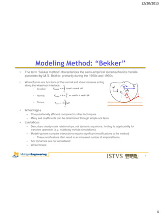
Bekker Parameter Identification
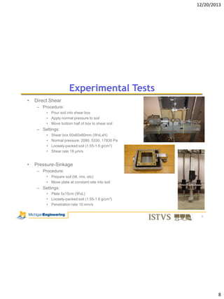
Direct Shear:
• Bekker parameters c, ϕ, and K were determined by
numerically minimizing the error given by:
2
arg min
j
c
tan
1 exp
c, ,K
j
K
Pressure-Sinkage:
• Bekker parameters k, and n were determined by
numerically minimizing the error given by:
n
arg min
z
k ,n
k
z
2
bplate
Parameter
Value
c [Pa]
139.280
ϕ [rad]
0.606
K [m]
5.151x10⁻⁴
k [Pa]
2.541x10⁵
n [-]
1.387
9
9](https://image.slidesharecdn.com/paper815830-140206132309-phpapp01/85/Comparison-of-DEM-and-Traditional-Modeling-Methods-for-Simulating-Steady-State-Wheel-Terrain-Interaction-for-Small-Vehicles-Paper81583-9-320.jpg)
![12/20/2013
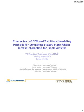
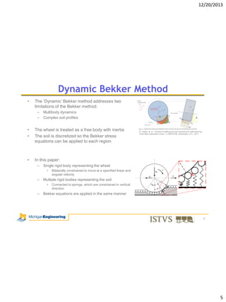
DEM Direct Shear Tests
•
•
•
Same shear box dimensions as experimental
Normal pressure applied by using a rigid body of
closely-packed particles with necessary density
Increased shear rate required to limit computation
cost
– Reducing the shear rate further had negligible
impact on simulation results
•
Computation Time:
– Simulations were run on a single core of an Intel
Xeon 5160 (3.0 GHz), at a rate of 40 to 20 cpu
minutes per simulation second for time steps 1.5
and 3.8 μs, respectively
Parameter
shear box dimensions [mm]
normal load [Pa]
shear rate [mm/s]
shear displacement [mm]
number of soil particles
time step [sec]
Value
60 x 60 x 60 (W x L x H)
2080, 5330, 17830
0.66
6.6
~640
1.5 - 3.8x10⁻⁶
10
10](https://image.slidesharecdn.com/paper815830-140206132309-phpapp01/85/Comparison-of-DEM-and-Traditional-Modeling-Methods-for-Simulating-Steady-State-Wheel-Terrain-Interaction-for-Small-Vehicles-Paper81583-10-320.jpg)
![12/20/2013
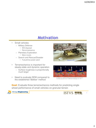
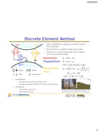
DEM Pressure-Sinkage Tests
•
•
Same size plate dimensions as experimental
Soil bin was 3x size of plate (recommended by
MIT to limit edge effects)
– Periodic boundaries used to further remove wall
effects
•
Same sinkage rate as experimental
•
Computation Time:
– Simulations were run on a single core of an Intel
Xeon 5160 (3.0 GHz), at a rate of 6 to 3 hours
cpu per simulation second for time steps 1.5 and
3.8 μs, respectively
Parameter
soil bin dimensions [mm]
plate dimensions [mm]
sinkage rate [mm/s]
maximum sinkage [mm]
number of soil particles
time step [sec]
Value
150 x 400 x 160
(W x L x H)
50 x 130 x 10
(W x L x H)
10.0
20.0
~30,000
1.5 - 3.8x10⁻⁶
11
11](https://image.slidesharecdn.com/paper815830-140206132309-phpapp01/85/Comparison-of-DEM-and-Traditional-Modeling-Methods-for-Simulating-Steady-State-Wheel-Terrain-Interaction-for-Small-Vehicles-Paper81583-11-320.jpg)
![12/20/2013
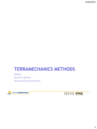
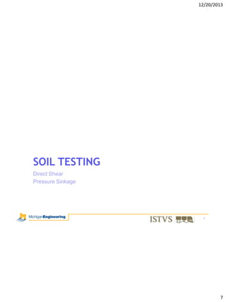
New Rolling Resistance Model
•
The direct-shear and pressure-sinkage soil
tests have widely different shear/sinkage
rates
–
–
•
–
Increasing drag force when velocity increased
from 1 to 50 mm/s [1]
DEM pile formation simulations found rolling
friction depended on the relative motion
between particles [2]
Rolling Resistance Torque
Tr
min Trk
Tr,k t+
Shear rate 18 μm/s
Penetration rate 10 mm/s
The properties of granular soil have been
shown to be rate dependent
–
•
t
Tr,k t
Ri
Rj
Fn
ΔTrk
k r Δθr
Spring/Damper Components
kr
r
•
r, eff
r Δωr
Tr
ΔTrk
•
Ri R j
Tr ,
2.25k n
Ri R j
r, eff
Ri
2
Rj
2 k r I eff
Coefficients
I eff
r, eff
1.4
M i Ri2 M j R j2
M i Ri2
min
M j R j2
2
r
vt , 1.0
[1] B. Yeomans, C. M. Saaj, and M. Van Winnendael, “Walking
planetary rovers – Experimental analysis and modelling of leg thrust
in loose granular soils,” J. Terramechanics, vol. 50, no. 2, pp. 107–
120, Apr. 2013.
[2] A. P. Grima and P. W. Wypych, “Discrete element simulations of
granular pile formation: Method for calibrating discrete element
models,” Eng. Comput., vol. 28, no. 3, pp. 314–339, 2011.
12
12](https://image.slidesharecdn.com/paper815830-140206132309-phpapp01/85/Comparison-of-DEM-and-Traditional-Modeling-Methods-for-Simulating-Steady-State-Wheel-Terrain-Interaction-for-Small-Vehicles-Paper81583-12-320.jpg)

![12/20/2013
Settings: Bekker Method
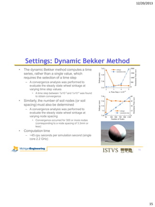
•
Some of the Bekker parameters cannot be determined from soil tests
– Parameters a0 and a1 used to determine the location of maximum shear stress
– These parameters can only be determined experimentally using wheel tests
Parameter
a0 [-]
a1 [-]
θr [rad]
•
Value
0.18
0.32
0
Parameter values were chosen assuming coefficients from the literature
– The goal is to predict, not to fit, wheel performance
J. Wong and A. Reece, “Prediction of rigid wheel performance based on the analysis of soil-wheel stresses part I.
Performance of driven rigid wheels,” J. Terramechanics, vol. 4, pp. 81–98, 1967.
•
Computation time
– ~43 ms to solve for a given slip ratio and normal load (using standard iterative
solving method, implemented in C)
14
14](https://image.slidesharecdn.com/paper815830-140206132309-phpapp01/85/Comparison-of-DEM-and-Traditional-Modeling-Methods-for-Simulating-Steady-State-Wheel-Terrain-Interaction-for-Small-Vehicles-Paper81583-14-320.jpg)
![12/20/2013
Settings: DEM
•
DEM wheel composed of 1cm diameter
overlapping particles, grouped to act as a
single rigid body
•
Experimental wheel/soil bin dimensions
were maintained
•
Procedure:
– Wheel placed on soil, allowed to rest for 0.5
seconds
– An x-axis force and a y-axis torque were
applied to the wheel for 1 second to ramp-up
the longitudinal and angular velocities
– Wheel was simulated for a distance of 0.7m,
or until steady-state was reached
•
Parameter
soil bed dimensions [mm]
number of soil particles
number of wheel particles
time step [sec]
Value
600 x 1000 x 160
(W x L x H)
~300,000
~12,000
2.2x10⁻⁶
Computation time
– ~8.5 cpu hours per simulation second (8
cores 3.0 GHz)
16
16](https://image.slidesharecdn.com/paper815830-140206132309-phpapp01/85/Comparison-of-DEM-and-Traditional-Modeling-Methods-for-Simulating-Steady-State-Wheel-Terrain-Interaction-for-Small-Vehicles-Paper81583-16-320.jpg)
![12/20/2013
DEM-Tuned Bekker Method
•
•
Bekker parameters can be tuned to produce similar results as DEM
When the Bekker method capabilities are sufficient, may be able to tune to DEM
simulations
Parameter
c [Pa]
ϕ [rad]
K [m]
k [Pa]
n [-]
a0 [-]
a1 [-]
θr [rad]
Soil-Tuned Values
139.280
0.606
5.151x10⁻⁴
2.541x10⁵
1.387
0.18*
0.32*
0
DEM-Tuned Values
96.240
0.606
4.534x10⁻³
2.305x10⁴
0.418
0.09
0.90
0
21
21](https://image.slidesharecdn.com/paper815830-140206132309-phpapp01/85/Comparison-of-DEM-and-Traditional-Modeling-Methods-for-Simulating-Steady-State-Wheel-Terrain-Interaction-for-Small-Vehicles-Paper81583-21-320.jpg)

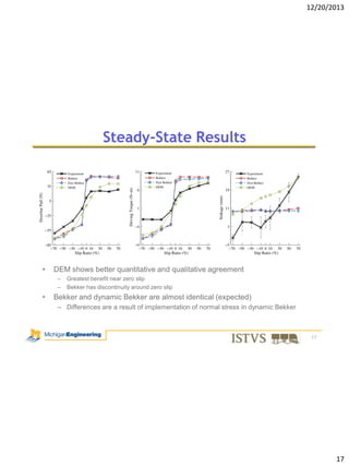
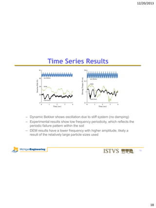
This document discusses the comparison of various terramechanics modeling methods, specifically the Bekker method, Dynamic Bekker method, and Discrete Element Method (DEM), for simulating wheel-terrain interaction in small vehicles. It highlights the advantages and limitations of each method, including computational efficiency and prediction accuracy for wheel performance on granular terrain. Experimental procedures and parameter identification for soil testing are also detailed to support the evaluation of these modeling techniques.