Operating Systems (slides)

Operating System
Introduction
Wang Xiaolin
April 9, 2016
u wx672ster+os@gmail.com
1 / 397

Textbooks
D.P. Bovet and M. Cesatı́. Understanding The Linux
Kernel. 3rd ed. O’Reilly, 2005.
Silberschatz, Galvin, and Gagne. Operating System
Concepts Essentials. John Wiley & Sons, 2011.
Andrew S. Tanenbaum. Modern Operating Systems. 3rd.
Prentice Hall Press, 2007.
邹恒明. 计算机的心智：操作系统之哲学原理. 机械工业出版社,
2009.
2 / 397

Course Web Site
Course web site: http://cs2.swfu.edu.cn/moodle
Lecture slides:
http://cs2.swfu.edu.cn/∼wx672/lecture_notes/os/slides/
Source code: http://cs2.swfu.edu.cn/∼wx672/lecture_notes/os/src/
Sample lab report:
http://cs2.swfu.edu.cn/∼wx672/lecture_notes/os/sample-
report/
3 / 397

What’s an Operating System?
▶ “Everything a vendor ships when you order an operating
system”
▶ It’s the program that runs all the time
▶ It’s a resource manager
- Each program gets time with the resource
Each program gets space on the resource
▶ It’s a control program
- Controls execution of programs to prevent errors and
improper use of the computer
▶ No universally accepted deﬁnition
4 / 397

What’s in the OS?
Hardware
Hardware control
Device drivers
Character
devices
Block
devices
Buﬀer
cache
File subsystem
VFS
NFS · · · Ext2 VFAT
Process control
subsystem
Inter-process
communication
Scheduler
Memory
management
System call interface
Libraries
Kernel level
Hardware level
User level
Kernel level
User programs
trap
trap
5 / 397

Abstractions
To hide the complexity of the actual implementations
Section 1.10 Summary 25
o
-
to
e
Main memory I/O devicesProcessorOperating system
Processes
Virtual memory
Files
Virtual machine
Instruction set
architecture
one instruction at a time. The underlying hardware is far
ing multiple instructions in parallel, but always in a way
he simple, sequential model. By keeping the same execu-
rocessor implementations can execute the same machine 6 / 397

System Goals
Convenient vs. Efficient
▶ Convenient for the user — for PCs
▶ Efficient — for mainframes, multiusers
▶ UNIX
- Started with keyboard + printer, none paid to convenience
- Now, still concentrating on efficiency, with GUI support
7 / 397

History of Operating Systems
1401 7094 1401
(a) (b) (c) (d) (e) (f)
Card
reader
Tape
drive Input
tape
Output
tape
System
tape
Printer
Fig. 1-2. An early batch system. (a) Programmers bring cards to
1401. (b) 1401 reads batch of jobs onto tape. (c) Operator carries
input tape to 7094. (d) 7094 does computing. (e) Operator carries
output tape to 1401. (f) 1401 prints output.
8 / 397

1945 - 1955 First generation
- vacuum tubes, plug boards
1955 - 1965 Second generation
- transistors, batch systems
1965 - 1980 Third generation
- ICs and multiprogramming
1980 - present Fourth generation
- personal computers
9 / 397

Multi-programming is the ﬁrst instance where the
OS must make decisions for the users
Job scheduling — decides which job should be loaded into
the memory.
Memory management — because several programs in
memory at the same time
CPU scheduling — choose one job among all the jobs are
ready to run
Process management — make sure processes don’t oﬀend
each other
Job 3
Job 2
Job 1
Operating
system
Memory
partitions
10 / 397

The Operating System Zoo
▶ Mainframe OS
▶ Server OS
▶ Multiprocessor OS
▶ Personal computer OS
▶ Real-time OS
▶ Embedded OS
▶ Smart card OS
11 / 397

OS Services
Like a government
Helping the users:
▶ User interface
▶ Program execution
▶ I/O operation
▶ File system manipulation
▶ Communication
▶ Error detection
Keeping the system eﬃcient:
▶ Resource allocation
▶ Accounting
▶ Protection and security
12 / 397

A Computer System
Banking
system
Airline
reservation
Operating system
Web
browser
Compilers Editors
Application programs
Hardware
System
programs
Command
interpreter
Machine language
Microarchitecture
Physical devices
Fig. 1-1. A computer system consists of hardware, system pro-
13 / 397

CPU Working Cycle
Fetch
unit
Decode
unit
Execute
unit
1. Fetch the ﬁrst instruction from memory
2. Decode it to determine its type and operands
3. execute it
Special CPU Registers
Program counter(PC): keeps the memory address of the next
instruction to be fetched
Stack pointer(SP): points to the top of the current stack in
memory
Program status(PS): holds
- condition code bits
- processor state
14 / 397

System Bus
Monitor
Keyboard
Floppy
disk drive
Hard
disk drive
Hard
disk
controller
Floppy
disk
controller
Keyboard
controller
Video
controller
MemoryCPU
Bus
Fig. 1-5. Some of the components of a simple personal computer.
Address Bus: speciﬁes the memory locations (addresses) for
the data transfers
Data Bus: holds the data transfered. bidirectional
Control Bus: contains various lines used to route timing and
control signals throughout the system
15 / 397

Controllers and Peripherals
▶ Peripherals are real devices controlled by controller chips
▶ Controllers are processors like the CPU itself, have
control registers
▶ Device driver writes to the registers, thus control it
▶ Controllers are connected to the CPU and to each other
by a variety of buses
16 / 397

ISA
bridge
Modem
Mouse
PCI
bridgeCPU
Main
memory
SCSI USB
Local bus
Sound
card
Printer Available
ISA slot
ISA bus
IDE
disk
Available
PCI slot
Key-
board
Mon-
itor
Graphics
adaptor
Level 2
cache
Cache bus Memory bus
PCI bus
17 / 397

Motherboard Chipsets
Intel Core 2
(CPU)
Front
Side
Bus
North bridge
Chip
DDR2System RAM Graphics Card
DMI
Interface
South bridge
Chip
Serial ATA Ports Clock Generation
BIOS
USB Ports
Power Management
PCI Bus
18 / 397

▶ The CPU doesn’t know what it’s connected to
- CPU test bench? network router? toaster? brain
implant?
▶ The CPU talks to the outside world through its pins
- some pins to transmit the physical memory address
- other pins to transmit the values
▶ The CPU’s gateway to the world is the front-side bus
Intel Core 2 QX6600
▶ 33 pins to transmit the physical memory address
- so there are 233
choices of memory locations
▶ 64 pins to send or receive data
- so data path is 64-bit wide, or 8-byte chunks
This allows the CPU to physically address 64GB of memory
(233
× 8B)
19 / 397

the northbridge
1. receives a physical memory request
2. decides where to route it
- to RAM? to video card? to ...?
- decision made via the memory address map
21 / 397

Bootstrapping
Can you pull yourself up by your own bootstraps?
A computer cannot run without ﬁrst loading software but
must be running before any software can be loaded.
BIOS
Initialization
MBR Boot Loader
Earily
Kernel
Initialization
Full
Kernel
Initialization
First
User Mode
Process
BIOS Services Kernel Services
Hardware
CPU in Real Mode
Time ﬂow
CPU in Protected Mode
Switch to
Protected Mode
22 / 397

Intel x86 Bootstrapping
1. BIOS (0xfffffff0)
« POST « HW init « Find a boot device (FD,CD,HD...) «
Copy sector zero (MBR) to RAM (0x00007c00)
2. MBR – the ﬁrst 512 bytes, contains
▶ Small code (< 446 Bytes), e.g. GRUB stage 1, for loading
GRUB stage 2
▶ the primary partition table (= 64 Bytes)
▶ its job is to load the second-stage boot loader.
3. GRUB stage 2 — load the OS kernel into RAM
4. startup
5. init — the ﬁrst user-space program
|<-------------Master Boot Record (512 Bytes)------------>|
0 439 443 445 509 511
+----//-----+----------+------+------//---------+---------+
| code area | disk-sig | null | partition table | MBR-sig |
| 440 | 4 | 2 | 16x4=64 | 0xAA55 |
+----//-----+----------+------+------//---------+---------+
$ sudo hd -n512 /dev/sda
23 / 397

Why Interrupt?
While a process is reading a disk ﬁle, can we do...
while(!done_reading_a_file())
{
let_CPU_wait();
// or...
lend_CPU_to_others();
}
operate_on_the_file();
24 / 397

Modern OS are Interrupt Driven
HW INT by sending a signal to CPU
SW INT by executing a system call
Trap (exception) is a software-generated INT coursed by an
error or by a speciﬁc request from an user
program
Interrupt vector is an array of pointers pointing to the
memory addresses of interrupt handlers. This
array is indexed by a unique device number
$ less /proc/devices
$ less /proc/interrupts
25 / 397

Programmable Interrupt Controllers
Interrupt
INT
IRQ 0 (clock)
IRQ 1 (keyboard)
IRQ 3 (tty 2)
IRQ 4 (tty 1)
IRQ 5 (XT Winchester)
IRQ 6 (floppy)
IRQ 7 (printer)
IRQ 8 (real time clock)
IRQ 9 (redirected IRQ 2)
IRQ 10
IRQ 11
IRQ 12
IRQ 13 (FPU exception)
IRQ 14 (AT Winchester)
IRQ 15
ACK
Master
interrupt
controller
INT
ACK
Slave
interrupt
controller
INT
CPU
INTA
Interrupt
ack
s
y
s
t
^
e
m
d
a
t
^
a
b
u
s
Figure 2-33. Interrupt processing hardware on a 32-bit Intel PC.
26 / 397

Interrupt Processing
CPU
Interrupt
controller
Disk
controller
Disk drive
Current instruction
Next instruction
1. Interrupt
3. Return
2. Dispatch
to handler
Interrupt handler
(b)(a)
1
3
4 2
Fig. 1-10. (a) The steps in starting an I/O device and getting an
interrupt. (b) Interrupt processing involves taking the interrupt,
running the interrupt handler, and returning to the user program.
27 / 397

Interrupt Timeline
1.2 Computer-System Organization 9
user
process
executing
CPU
I/O interrupt
processing
I/O
request
transfer
done
I/O
request
transfer
done
I/O
device
idle
transferring
Figure 1.3 Interrupt time line for a single process doing output.
the interrupting device. Operating systems as different as Windows and UNIX
dispatch interrupts in this manner. 28 / 397

System Calls
A System Call
▶ is how a program requests a service from an OS kernel
▶ provides the interface between a process and the OS
29 / 397

Program 1 Program 2 Program 3
+---------+ +---------+ +---------+
| fork() | | vfork() | | clone() |
+---------+ +---------+ +---------+
| | |
+--v-----------v-----------v--+
| C Library |
+--------------o--------------+ User space
-----------------|------------------------------------
+--------------v--------------+ Kernel space
| System call |
+--------------o--------------+
| +---------+
| : ... :
| 3 +---------+ sys_fork()
o------>| fork() |---------------.
| +---------+ |
| : ... : |
| 120 +---------+ sys_clone() |
o------>| clone() |---------------o
| +---------+ |
| : ... : |
| 289 +---------+ sys_vfork() |
o------>| vfork() |---------------o
+---------+ |
: ... : v
+---------+ do_fork()
System Call Table 30 / 397

User program 2

User program 1

Kernel call
Service

procedure

Dispatch table

User programs

run in
user mode

Operating

system

runs in

kernel mode
4

3

1
2

Mainmemory
Figure 1-16. How a system call can be made: (1) User pro-
gram traps to the kernel. (2) Operating system determines ser-
vice number required. (3) Operating system calls service pro-
cedure. (4) Control is returned to user program.
31 / 397

The 11 steps in making the system call
read(fd,buffer,nbytes)
Return to caller
4
10
6
0
9
7 8
3
2
1
11
Dispatch
Sys call
handler
Address
0xFFFFFFFF
User space
Kernel space
(Operating system)
Library
procedure
read
User program
calling read
Trap to the kernel
Put code for read in register
Increment SP
Call read
Push fd
Push buffer
Push nbytes
5
32 / 397

Process management
Call Description
pid = fork( ) Create a child process identical to the parent
pid = waitpid(pid, statloc, options) Wait for a child to terminate
s = execve(name, argv, environp) Replace a process’ core image
exit(status) Terminate process execution and return status
File management
Call Description
fd = open(file, how, ...) Open a file for reading, writing or both
s = close(fd) Close an open file
n = read(fd, buffer, nbytes) Read data from a file into a buffer
n = write(fd, buffer, nbytes) Write data from a buffer into a file
position = lseek(fd, offset, whence) Move the file pointer
s = stat(name, buf) Get a file’s status information
Directory and file system management
Call Description
s = mkdir(name, mode) Create a new directory
s = rmdir(name) Remove an empty directory
s = link(name1, name2) Create a new entry, name2, pointing to name1
s = unlink(name) Remove a directory entry
s = mount(special, name, flag) Mount a file system
s = umount(special) Unmount a file system
Miscellaneous
Call Description
s = chdir(dirname) Change the working directory
s = chmod(name, mode) Change a file’s protection bits
s = kill(pid, signal) Send a signal to a process
seconds = time(seconds) Get the elapsed time since Jan. 1, 1970
33 / 397

System Call Examples
fork()
1 #include stdio.h
2 #include unistd.h
3
4 int main ()
5 {
6 printf(Hello World!n);
7 fork();
8 printf(Goodbye Cruel World!n);
9 return 0;
10 }
$ man 2 fork
34 / 397

exec()
1 #include stdio.h
2 #include unistd.h
3
4 int main ()
5 {
7 if(fork() != 0 )
8 printf(I am the parent process.n);
9 else {
10 printf(A child is listing the directory contents...n);
11 execl(/bin/ls, ls, -al, NULL);
12 }
13 return 0;
14 }
$ man 3 exec
35 / 397

Hardware INT vs. Software INT
Device:
Send electrical signal to interrupt controller.
Controller:
1. Interrupt CPU.
2. Send digital identification of interrupting
device.
Kernel:
1. Save registers.
2. Execute driver software to read I/O device.
3. Send message.
4. Restart a process (not necessarily
interrupted process).
Caller:
1. Put message pointer and destination of
message into CPU registers.
2. Execute software interrupt instruction.
Kernel:
1. Save registers.
2. Send and/or receive message.
3. Restart a process (not necessarily calling
process).
(a) (b)
Figure 2-34. (a) How a hardware interrupt is processed. (b)
How a system call is made.
36 / 397

References
Wikipedia. Interrupt — Wikipedia, The Free
Encyclopedia. [Online; accessed 21-February-2015].
2015.
Wikipedia. System call — Wikipedia, The Free
2015.
37 / 397

Processes Threads
Wang Xiaolin
April 9, 2016
38 / 397

Process
A process is an instance of a program in execution
Processes are like human beings:
« they are generated
« they have a life
« they optionally generate one or
more child processes, and
« eventually they die
A small diﬀerence:
▶ sex is not really common among
processes
▶ each process has just one parent
Stack
Gap
Data
Text
0000
FFFF
39 / 397

Process Control Block (PCB)
Implementation
A process is the collection of data
structures that fully describes how far the
execution of the program has progressed.
▶ Each process is represented by a PCB
▶ task_struct in
+-------------------+
| process state |
+-------------------+
| PID |
+-------------------+
| program counter |
+-------------------+
| registers |
+-------------------+
| memory limits |
+-------------------+
| list of open files|
+-------------------+
| ... |
+-------------------+
40 / 397

Process Creation
exit()exec()
fork() wait()
anything()
parent
child
▶ When a process is created, it is almost identical to its
parent
▶ It receives a (logical) copy of the parent’s address space,
and
▶ executes the same code as the parent
▶ The parent and child have separate copies of the data
(stack and heap)
41 / 397

Forking in C
1 #include stdio.h
2 #include unistd.h
3
4 int main ()
5 {
7 fork();
8 printf(Goodbye Cruel World!n);
9 return 0;
10 }
$ man fork
42 / 397

exec()
1 int main()
2 {
3 pid_t pid;
4 /* fork another process */
5 pid = fork();
6 if (pid 0) { /* error occurred */
7 fprintf(stderr, Fork Failed);
8 exit(-1);
9 }
10 else if (pid == 0) { /* child process */
11 execlp(/bin/ls, ls, NULL);
12 }
13 else { /* parent process */
14 /* wait for the child to complete */
15 wait(NULL);
16 printf (Child Complete);
17 exit(0);
18 }
19 return 0;
20 }
$ man 3 exec
43 / 397

Process State Transition
1 23
4
Blocked
Running
Ready
1. Process blocks for input
2. Scheduler picks another process
3. Scheduler picks this process
4. Input becomes available
Fig. 2-2. A process can be in running, blocked, or ready state.
Transitions between these states are as shown.
44 / 397

CPU Switch From Process To Process
45 / 397

Process vs. Thread
a single-threaded process = resource + execution
a multi-threaded process = resource + executions
Thread Thread
Kernel Kernel
Process 1 Process 1 Process 1 Process
User
space
Kernel
space
(a) (b)
Fig. 2-6. (a) Three processes each with one thread. (b) One process
with three threads.
A process = a unit of resource ownership, used to group
resources together;
A thread = a unit of scheduling, scheduled for execution
on the CPU.
46 / 397

Process vs. Thread
multiple threads running
in one process:
multiple processes run-
ning in one computer:
share an address space and
other resources
share physical memory,
disk, printers ...
No protection between threads
impossible — because process is the minimum unit of
resource management
unnecessary — a process is owned by a single user
47 / 397

A Multi-threaded Web Server
Dispatcher thread
Worker thread
Web page cache
Kernel
Network
connection
Web server process
User
space
Kernel
space
Fig. 2-10. A multithreaded Web server.
while (TRUE) { while (TRUE) {
get next request(buf); wait for work(buf)
handoff work(buf); look for page in cache(buf, page);
} if (page not in cache(page))
read page from disk(buf, page);
return page(page);
}
(a) (b)
49 / 397

A Word Processor With 3 Threads
Kernel
Keyboard Disk
Four score and seven
years ago, our fathers
brought forth upon this
continent a new nation:
conceived in liberty,
and dedicated to the
proposition that all
men are created equal.
Now we are engaged
in a great civil war
testing whether that
nation, or any nation
so conceived and so
dedicated, can long
endure. We are met on
a great battlefield of
that war.
We have come to
dedicate a portion of
that field as a final
resting place for those
who here gave their
lives that this nation
might live. It is
altogether fitting and
proper that we should
do this.
But, in a larger sense,
we cannot dedicate, we
cannot consecrate we
cannot hallow this
ground. The brave
men, living and dead,
who struggled here
have consecrated it, far
above our poor power
to add or detract. The
world will little note,
nor long remember,
what we say here, but
it can never forget
what they did here.
It is for us the living,
rather, to be dedicated
here to the unfinished
work which they who
fought here have thus
far so nobly advanced.
It is rather for us to be
here dedicated to the
great task remaining
before us, that from
these honored dead we
take increased devotion
to that cause for which
they gave the last full
measure of devotion,
that we here highly
resolve that these dead
shall not have died in
vain that this nation,
under God, shall have
a new birth of freedom
and that government of
the people by the
people, for the people
Fig. 2-9. A word processor with three threads.
50 / 397

Why Having a Kind of Process Within a Process?
▶ Responsiveness
▶ Good for interactive applications.
▶ A process with multiple threads makes a great server (e.g.
a web server):
Have one server process, many ”worker” threads – if one
thread blocks (e.g. on a read), others can still continue
executing
▶ Economy – Threads are cheap!
▶ Cheap to create – only need a stack and storage for
registers
▶ Use very little resources – don’t need new address space,
global data, program code, or OS resources
▶ switches are fast – only have to save/restore PC, SP, and
registers
▶ Resource sharing – Threads can pass data via shared
memory; no need for IPC
▶ Can take advantage of multiprocessors
51 / 397

Thread States Transition
Same as process states transition
1 23
4
Blocked
Running
Ready
1. Process blocks for input
2. Scheduler picks another process
3. Scheduler picks this process
4. Input becomes available
Fig. 2-2. A process can be in running, blocked, or ready state.
Transitions between these states are as shown.
52 / 397

Each Thread Has Its Own Stack
▶ A typical stack stores local data and call information for
(usually nested) procedure calls.
▶ Each thread generally has a diﬀerent execution history.
Kernel
Thread 3's stack
Process
Thread 3Thread 1
Thread 2
Thread 1's
stack
Fig. 2-8. Each thread has its own stack.
53 / 397

Thread Operations
Start
with one
thread
running
thread1
thread2
thread3
end
release
CPU
wait for
a thread
to exit
thread_create()
thread_create()
thread_create()
thread_exit()
thread_yield()
thread_exit()
thread_exit()
thread_join()
54 / 397

POSIX Threads
IEEE 1003.1c The standard for writing portable threaded
programs. The threads package it deﬁnes is
called Pthreads, including over 60 function calls,
supported by most UNIX systems.
Some of the Pthreads function calls
Thread call Description
pthread_create Create a new thread
pthread_exit Terminate the calling thread
pthread_join Wait for a speciﬁc thread to exit
pthread_yield Release the CPU to let another
thread run
pthread_attr_init Create and initialize a thread’s at-
tribute structure
pthread_attr_destroy Remove a thread’s attribute struc-
ture
55 / 397

Pthreads
Example 1
1 #include pthread.h
2 #include stdlib.h
3 #include unistd.h
4 #include stdio.h
5
6 void *thread_function(void *arg){
7 int i;
8 for( i=0; i20; i++ ){
9 printf(Thread says hi!n);
10 sleep(1);
11 }
12 return NULL;
13 }
14
15 int main(void){
16 pthread_t mythread;
17 if(pthread_create(mythread, NULL, thread_function, NULL)){
18 printf(error creating thread.);
19 abort();
20 }
21
22 if(pthread_join(mythread, NULL)){
23 printf(error joining thread.);
24 abort();
25 }
26 exit(0);
27 }
56 / 397

Pthreads
pthread_t deﬁned in pthread.h, is often called a ”thread id”
(tid);
pthread_create() returns zero on success and a non-zero
value on failure;
pthread_join() returns zero on success and a non-zero value
on failure;
How to use pthread?
1. #includepthread.h
2. $ gcc thread1.c -o thread1 -pthread
3. $ ./thread1
57 / 397

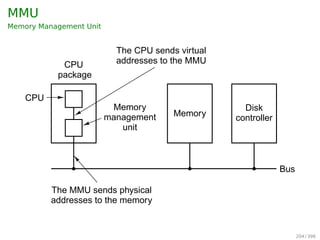
Pthreads
Example 2
1 #include pthread.h
2 #include stdio.h
3 #include stdlib.h
4
5 #define NUMBER_OF_THREADS 10
6
7 void *print_hello_world(void *tid)
8 {
9 /* prints the thread’s identifier, then exits.*/
10 printf (Thread %d: Hello World!n, tid);
11 pthread_exit(NULL);
12 }
13
14 int main(int argc, char *argv[])
15 {
16 pthread_t threads[NUMBER_OF_THREADS];
17 int status, i;
18 for (i=0; iNUMBER_OF_THREADS; i++)
19 {
20 printf (Main: creating thread %dn,i);
21 status = pthread_create(threads[i], NULL, print_hello_world, (void *)i);
22
23 if(status != 0){
24 printf (Oops. pthread_create returned error code %dn,status);
25 exit(-1);
26 }
27 }
28 exit(NULL);
29 }
58 / 397

Pthreads
With or without pthread_join()? Check it by yourself.
59 / 397

User-Level Threads vs. Kernel-Level Threads
Process ProcessThread Thread
Process
table
Process
table
Thread
table
Thread
table
Run-time
system
Kernel
space
User
space
KernelKernel
Fig. 2-13. (a) A user-level threads package. (b) A threads package
managed by the kernel.
60 / 397

User-Level Threads
User-level threads provide a library of functions to allow user
processes to create and manage their own
threads.
No need to modify the OS;
Simple representation
▶ each thread is represented simply by a PC, regs, stack, and
a small TCB, all stored in the user process’ address space
Simple Management
▶ creating a new thread, switching between threads, and
synchronization between threads can all be done without
intervention of the kernel
Fast
▶ thread switching is not much more expensive than a
procedure call
Flexible
▶ CPU scheduling (among threads) can be customized to suit
the needs of the algorithm – each process can use a
diﬀerent thread scheduling algorithm
61 / 397

User-Level Threads
Lack of coordination between threads and OS kernel
▶ Process as a whole gets one time slice
▶ Same time slice, whether process has 1 thread or 1000
threads
▶ Also – up to each thread to relinquish control to other
threads in that process
Requires non-blocking system calls (i.e. a multithreaded
kernel)
▶ Otherwise, entire process will blocked in the kernel, even if
there are runnable threads left in the process
▶ part of motivation for user-level threads was not to have to
modify the OS
If one thread causes a page fault(interrupt!), the entire
process blocks
62 / 397

Kernel-Level Threads
Kernel-level threads kernel provides system calls to create
and manage threads
Kernel has full knowledge of all threads
▶ Scheduler may choose to give a process with 10 threads
more time than process with only 1 thread
Good for applications that frequently block (e.g. server
processes with frequent interprocess communication)
Slow – thread operations are 100s of times slower than
for user-level threads
Signiﬁcant overhead and increased kernel complexity –
kernel must manage and schedule threads as well as
processes
▶ Requires a full thread control block (TCB) for each thread
63 / 397

Hybrid Implementations
Combine the advantages of two
Multiple user threads
on a kernel thread
User
space
Kernel
spaceKernel threadKernel
Fig. 2-14. Multiplexing user-level threads onto kernel-level
threads. 64 / 397

Programming Complications
▶ fork(): shall the child has the threads that its parent
has?
▶ What happens if one thread closes a ﬁle while another is
still reading from it?
▶ What happens if several threads notice that there is too
little memory?
And sometimes, threads ﬁx the symptom, but not the
problem.
65 / 397

Linux Threads
To the Linux kernel, there is no concept of a thread
▶ Linux implements all threads as standard processes
▶ To Linux, a thread is merely a process that shares certain
resources with other processes
▶ Some OS (MS Windows, Sun Solaris) have cheap threads
and expensive processes.
▶ Linux processes are already quite lightweight
On a 75MHz Pentium
thread: 1.7µs
fork: 1.8µs
66 / 397

Linux Threads
clone() creates a separate process that shares the address
space of the calling process. The cloned task behaves
much like a separate thread.
Program 3
Kernel space
User space
fork()
clone()
vfork()
System Call Table
3
120
289
Program 1 Program 2
C Library
vfork()fork() clone()
System call sys_fork()
sys_clone()
sys_vfork()
do_fork()
67 / 397

clone()
1 #include sched.h
2 int clone(int (*fn) (void *), void *child_stack,
3 int flags, void *arg, ...);
arg 1 the function to be executed, i.e. fn(arg), which
returns an int;
arg 2 a pointer to a (usually malloced) memory space to be
used as the stack for the new thread;
arg 3 a set of ﬂags used to indicate how much the calling
process is to be shared. In fact,
clone(0) == fork()
arg 4 the arguments passed to the function.
It returns the PID of the child process or -1 on failure.
$ man clone
68 / 397

The clone() System Call
Some flags:
flag Shared
CLONE_FS File-system info
CLONE_VM Same memory space
CLONE_SIGHAND Signal handlers
CLONE_FILES The set of open files
In practice, one should try to avoid calling clone()
directly
Instead, use a threading library (such as pthreads) which
use clone() when starting a thread (such as during a call
to pthread_create())
69 / 397

clone() Example
1 #include unistd.h
2 #include sched.h
3 #include sys/types.h
4 #include stdlib.h
5 #include string.h
6 #include stdio.h
7 #include fcntl.h
8
9 int variable;
10
11 int do_something()
12 {
13 variable = 42;
14 _exit(0);
15 }
16
17 int main(void)
18 {
19 void *child_stack;
20 variable = 9;
21
22 child_stack = (void *) malloc(16384);
23 printf(The variable was %dn, variable);
24
25 clone(do_something, child_stack,
26 CLONE_FS | CLONE_VM | CLONE_FILES, NULL);
27 sleep(1);
28
29 printf(The variable is now %dn, variable);
30 return 0;
31 } 70 / 397

clone() Example
1 #include unistd.h
2 #include sched.h
3 #include sys/types.h
4 #include stdlib.h
5 #include string.h
6 #include stdio.h
7 #include fcntl.h
8
9 int variable;
10
11 int do_something()
12 {
13 variable = 42;
14 _exit(0);
15 }
16
17 int main(void)
18 {
19 void *child_stack;
20 variable = 9;
21
22 child_stack = (void *) malloc(16384);
23 printf(The variable was %dn, variable);
24
25 clone(do_something, child_stack,
26 CLONE_FS | CLONE_VM | CLONE_FILES, NULL);
27 sleep(1);
28
29 printf(The variable is now %dn, variable);
30 return 0;
31 }

70 / 397

Stack Grows Downwards
child_stack = (void**)malloc(8192) + 8192/sizeof(*child_stack);
✓
71 / 397

References
Wikipedia. Process (computing) — Wikipedia, The Free
2014.
Wikipedia. Process control block — Wikipedia, The Free
2015.
Wikipedia. Thread (computing) — Wikipedia, The Free
2015.
72 / 397

Process Synchronization
Wang Xiaolin
April 9, 2016
73 / 397

Interprocess Communication
Example:
ps | head -2 | tail -1 | cut -f2 -d' '
IPC issues:
1. How one process can pass information to another
2. Be sure processes do not get into each other’s way
e.g. in an airline reservation system, two processes compete
for the last seat
3. Proper sequencing when dependencies are present
e.g. if A produces data and B prints them, B has to wait until A
has produced some data
Two models of IPC:
▶ Shared memory
▶ Message passing (e.g. sockets)
74 / 397

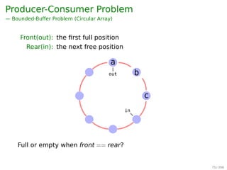
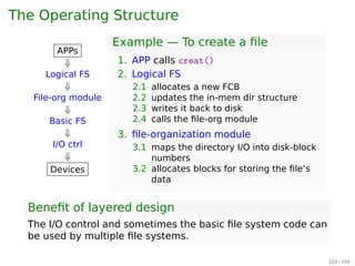
Producer-Consumer Problem
compiler Assembly
code assembler
Object
module loader
Process
wants
printing
file
Printer
daemon
75 / 397

Process Synchronization
▶ Consumers don’t try to remove objects from Buffer when
it is empty.
▶ Producers don’t try to add objects to the Buffer when it is
full.
Producer
1 while(TRUE){
2 while(FULL);
3 item = produceItem();
4 insertItem(item);
5 }
Consumer
1 while(TRUE){
2 while(EMPTY);
3 item = removeItem();
4 consumeItem(item);
5 }
How to define full/empty?
76 / 397

— Bounded-Buﬀer Problem (Circular Array)
Front(out): the ﬁrst full position
Rear(in): the next free position
out
in
c
b
a
Full or empty when front == rear?
77 / 397

Common solution:
Full: when (in+1)%BUFFER_SIZE == out
Actually, this is full - 1
Empty: when in == out
Can only use BUFFER_SIZE-1 elements
Shared data:
1 #define BUFFER_SIZE 6
2 typedef struct {
3 ...
4 } item;
5 item buffer[BUFFER_SIZE];
6 int in = 0; //the next free position
7 int out = 0;//the first full position
78 / 397

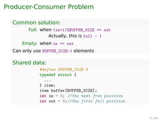
Bounded-Buﬀer Problem
Producer:
1 while (true) {
2 /* do nothing -- no free buffers */
3 while (((in + 1) % BUFFER_SIZE) == out);
4
5 buffer[in] = item;
6 in = (in + 1) % BUFFER_SIZE;
7 }
Consumer:
1 while (true) {
2 while (in == out); // do nothing
3 // remove an item from the buffer
4 item = buffer[out];
5 out = (out + 1) % BUFFER_SIZE;
6 return item;
7 }
out
in
c
b
a
79 / 397

Race Conditions
Now, let’s have two producers
4
5
6
7
abc
prog.c
prog.n
Process A
out = 4
in = 7
Process B
Spooler
directory
Fig. 2-18. Two processes want to access shared memory at the 80 / 397

Race Conditions
Two producers
1 #define BUFFER_SIZE 100
2 typedef struct {
3 ...
4 } item;
5 item buffer[BUFFER_SIZE];
6 int in = 0;
7 int out = 0;
Process A and B do the same thing:
1 while (true) {
2 while (((in + 1) % BUFFER_SIZE) == out);
3 buffer[in] = item;
4 in = (in + 1) % BUFFER_SIZE;
5 }
81 / 397

Race Conditions
Problem: Process B started using one of the shared
variables before Process A was ﬁnished with it.
Solution: Mutual exclusion. If one process is using a
shared variable or ﬁle, the other processes will
be excluded from doing the same thing.
82 / 397

Critical Regions
Mutual Exclusion
Critical Region: is a piece of code accessing a common
resource.
A enters critical region
A leaves critical region
B attempts to
enter critical
region
B enters
critical region
T1
T2
T3
T4
Process A
Process B
B blocked
B leaves
critical region
Time
Fig. 2-19. Mutual exclusion using critical regions. 83 / 397

Critical Region
A solution to the critical region problem must satisfy three
conditions:
Mutual Exclusion: No two process may be simultaneously
inside their critical regions.
Progress: No process running outside its critical region
may block other processes.
Bounded Waiting: No process should have to wait forever to
enter its critical region.
84 / 397

Mutual Exclusion With Busy Waiting
Disabling Interrupts
1 {
2 ...
3 disableINT();
4 critical_code();
5 enableINT();
6 ...
7 }
Problems:
▶ It’s not wise to give user process the power of turning oﬀ
INTs.
▶ Suppose one did it, and never turned them on again
▶ useless for multiprocessor system
Disabling INTs is often a useful technique within the kernel
itself but is not a general mutual exclusion mechanism for
user processes.
85 / 397

Lock Variables
1 int lock=0; //shared variable
2 {
3 ...
4 while(lock); //busy waiting
5 lock=1;
6 critical_code();
7 lock=0;
8 ...
9 }
Problem:
▶ What if an interrupt occurs right at line 5?
▶ Checking the lock again while backing from an interrupt?
86 / 397

Strict Alternation
Process 0
1 while(TRUE){
2 while(turn != 0);
3 critical_region();
4 turn = 1;
5 noncritical_region();
6 }
Process 1
1 while(TRUE){
2 while(turn != 1);
3 critical_region();
4 turn = 0;
5 noncritical_region();
6 }
Problem: violates condition-2
▶ One process can be blocked by another not in its critical
region.
▶ Requires the two processes strictly alternate in entering
their critical region.
87 / 397

Peterson’s Solution
int interest[0] = 0;
int interest[1] = 0;
int turn;
P0
1 interest[0] = 1;
2 turn = 1;
3 while(interest[1] == 1
4 turn == 1);
5 critical_section();
6 interest[0] = 0;
P1
1 interest[1] = 1;
2 turn = 0;
3 while(interest[0] == 1
4 turn == 0);
5 critical_section();
6 interest[1] = 0;
Wikipedia. Peterson’s algorithm — Wikipedia, The Free
2015.
88 / 397

Hardware Solution: The TSL Instruction
Lock the memory bus
enter region:
TSL REGISTER,LOCK | copy lock to register and set lock to 1
CMP REGISTER,#0 | was lock zero?
JNE enter region | if it was non zero, lock was set, so loop
RET | return to caller; critical region entered
leave region:
MOVE LOCK,#0 | store a 0 in lock
RET | return to caller
Fig. 2-22. Entering and leaving a critical region using the TSL
instruction.
89 / 397

Mutual Exclusion Without Busy Waiting
Sleep Wakeup
1 #define N 100 /* number of slots in the buffer */
2 int count = 0; /* number of items in the buffer */
1 void producer(){
2 int item;
3 while(TRUE){
4 item = produce_item();
5 if(count == N)
6 sleep();
7 insert_item(item);
8 count++;
9 if(count == 1)
10 wakeup(consumer);
11 }
12 }
1 void consumer(){
2 int item;
3 while(TRUE){
4 if(count == 0)
5 sleep();
6 item = rm_item();
7 count--;
8 if(count == N - 1)
9 wakeup(producer);
10 consume_item(item);
11 }
12 }
90 / 397

Mutual Exclusion Without Busy Waiting
Sleep Wakeup
2 int count = 0; /* number of items in the buffer */
1 void producer(){
2 int item;
3 while(TRUE){
4 item = produce_item();
5 if(count == N)
6 sleep();
8 count++;
9 if(count == 1)
10 wakeup(consumer);
11 }
12 }
1 void consumer(){
2 int item;
3 while(TRUE){
4 if(count == 0)
5 sleep();
6 item = rm_item();
7 count--;
8 if(count == N - 1)
9 wakeup(producer);
10 consume_item(item);
11 }
12 }
Deadlock!
90 / 397

Race Condition
Problem
1. Consumer is going to sleep upon seeing an empty buffer,
but INT occurs;
2. Producer inserts an item, increasing count to 1, then call
wakeup(consumer);
3. But the consumer is not asleep, though count was 0. So
the wakeup() signal is lost;
4. Consumer is back from INT remembering count is 0, and
goes to sleep;
5. Producer sooner or later will fill up the buffer and also
goes to sleep;
6. Both will sleep forever, and waiting to be waken up by
the other process. Deadlock!
91 / 397

Race Condition
Solution: Add a wakeup waiting bit
1. The bit is set, when a wakeup is sent to an awaken
process;
2. Later, when the process wants to sleep, it checks the bit
ﬁrst. Turns it oﬀ if it’s set, and stays awake.
What if many processes try going to sleep?
92 / 397

What is a Semaphore?
▶ A locking mechanism
▶ An integer or ADT
that can only be operated with:
Atomic Operations
P() V()
Wait() Signal()
Down() Up()
Decrement() Increment()
... ...
1 down(S){
2 while(S=0);
3 S--;
4 }
1 up(S){
2 S++;
3 }
More meaningful names:
▶ increment_and_wake_a_waiting_process_if_any()
▶ decrement_and_block_if_the_result_is_negative()
93 / 397

Semaphore
How to ensure atomic?
1. For single CPU, implement up() and down() as system
calls, with the OS disabling all interrupts while accessing
the semaphore;
2. For multiple CPUs, to make sure only one CPU at a time
examines the semaphore, a lock variable should be used
with the TSL instructions.
94 / 397

Semaphore is a Special Integer
A semaphore is like an integer, with three
diﬀerences:
1. You can initialize its value to any integer, but after that
the only operations you are allowed to perform are
increment (S++) and decrement (S- -).
2. When a thread decrements the semaphore, if the result
is negative (S ≤ 0), the thread blocks itself and cannot
continue until another thread increments the semaphore.
3. When a thread increments the semaphore, if there are
other threads waiting, one of the waiting threads gets
unblocked.
95 / 397

Why Semaphores?
We don’t need semaphores to solve synchronization
problems, but there are some advantages to using them:
▶ Semaphores impose deliberate constraints that help
programmers avoid errors.
▶ Solutions using semaphores are often clean and
organized, making it easy to demonstrate their
correctness.
▶ Semaphores can be implemented eﬃciently on many
systems, so solutions that use semaphores are portable
and usually eﬃcient.
96 / 397

The Simplest Use of Semaphore
Signaling
▶ One thread sends a signal to another thread to indicate
that something has happened
▶ it solves the serialization problem
Signaling makes it possible to guarantee that a section of
code in one thread will run before a section of code in
another thread
Thread A
1 statement a1
2 sem.signal()
Thread B
1 sem.wait()
2 statement b1
What’s the initial value of sem?
97 / 397

Semaphore
Rendezvous Puzzle
Thread A
1 statement a1
2 statement a2
Thread B
1 statement b1
2 statement b2
Q: How to guarantee that
1. a1 happens before b2, and
2. b1 happens before a2
a1 → b2; b1 → a2
Hint: Use two semaphores initialized to 0.
98 / 397

Thread A: Thread B:
Solution 1:
statement a1 statement b1
sem1.wait() sem1.signal()
sem2.signal() sem2.wait()
Solution 2:
sem2.signal() sem1.signal()
sem1.wait() sem2.wait()
Solution 3:
99 / 397

Thread A: Thread B:
Solution 1:
sem1.wait() sem1.signal()
sem2.signal() sem2.wait()
Solution 2:
Solution 3:
statement a2 statement b2Deadlock!
99 / 397

Mutex
▶ A second common use for semaphores is to enforce
mutual exclusion
▶ It guarantees that only one thread accesses the shared
variable at a time
▶ A mutex is like a token that passes from one thread to
another, allowing one thread at a time to proceed
Q: Add semaphores to the following example to enforce
mutual exclusion to the shared variable i.
Thread A: i++ Thread B: i++
Why? Because i++ is not atomic.
100 / 397

i++ is not atomic in assembly language
1 LOAD [i], r0 ;load the value of 'i' into
2 ;a register from memory
3 ADD r0, 1 ;increment the value
4 ;in the register
5 STORE r0, [i] ;write the updated
6 ;value back to memory
Interrupts might occur in between. So, i++ needs to be
protected with a mutex.
101 / 397

Mutex Solution
Create a semaphore named mutex that is initialized
to 1
1: a thread may proceed and access the shared variable
0: it has to wait for another thread to release the mutex
Thread A
1 mutex.wait()
2 i++
3 mutex.signal()
Thread B
1 mutex.wait()
2 i++
3 mutex.signal()
102 / 397

Multiplex — Without Busy Waiting
1 typedef struct{
2 int space; //number of free resources
3 struct process *P; //a list of queueing producers
4 struct process *C; //a list of queueing consumers
5 } semaphore;
6 semaphore S;
7 S.space = 5;
Producer
1 void down(S){
2 S.space--;
3 if(S.space == 4){
4 rmFromQueue(S.C);
5 wakeup(S.C);
6 }
7 if(S.space 0){
8 addToQueue(S.P);
9 sleep();
10 }
11 }
Consumer
1 void up(S){
2 S.space++;
3 if(S.space 5){
4 addToQueue(S.C);
5 sleep();
6 }
7 if(S.space = 0){
8 rmFromQueue(S.P);
9 wakeup(S.P);
10 }
11 }
if S.space 0,
S.space == Number of queueing producers
if S.space 5,
S.space == Number of queueing consumers + 5
103 / 397

Barrier
Barrier
Barrier
Barrier
A A A
B B B
C C
D D D
Time Time Time
Process
(a) (b) (c)
C
Fig. 2-30. Use of a barrier. (a) Processes approaching a barrier.
(b) All processes but one blocked at the barrier. (c) When the last
process arrives at the barrier, all of them are let through.
1. Processes approaching a barrier
2. All processes but one blocked at the barrier
3. When the last process arrives at the barrier, all of them
are let through
Synchronization requirement:
specific_task()
critical_point()
No thread executes critical_point() until after all threads
have executed specific_task().
104 / 397

Barrier Solution
1 n = the number of threads
2 count = 0
3 mutex = Semaphore(1)
4 barrier = Semaphore(0)
count: keeps track of how many threads have arrived
mutex: provides exclusive access to count
barrier: is locked (≤ 0) until all threads arrive
When barrier.value0,
barrier.value == Number of queueing processes
Solution 1
1 specific_task();
2 mutex.wait();
3 count++;
4 mutex.signal();
5 if (count n)
6 barrier.wait();
7 barrier.signal();
8 critical_point();
Solution 2
1 specific_task();
2 mutex.wait();
3 count++;
4 mutex.signal();
5 if (count == n)
6 barrier.signal();
7 barrier.wait();
8 critical_point();
105 / 397

Barrier Solution
1 n = the number of threads
2 count = 0
3 mutex = Semaphore(1)
4 barrier = Semaphore(0)
count: keeps track of how many threads have arrived
mutex: provides exclusive access to count
barrier: is locked (≤ 0) until all threads arrive
When barrier.value0,
barrier.value == Number of queueing processes
Solution 1
1 specific_task();
2 mutex.wait();
3 count++;
4 mutex.signal();
5 if (count n)
6 barrier.wait();
7 barrier.signal();
8 critical_point();
Solution 2
1 specific_task();
2 mutex.wait();
3 count++;
4 mutex.signal();
5 if (count == n)
6 barrier.signal();
7 barrier.wait();
8 critical_point();
Only one thread can pass the barrier!
✓Deadlock!
105 / 397

Barrier Solution
Solution 3
1 specific_task();
2
3 mutex.wait();
4 count++;
5 mutex.signal();
6
7 if (count == n)
8 barrier.signal();
9
10 barrier.wait();
11 barrier.signal();
12
13 critical_point();
Solution 4
1 specific_task();
2
3 mutex.wait();
4 count++;
5
6 if (count == n)
7 barrier.signal();
8
9 barrier.wait();
11 mutex.signal();
12
106 / 397

Barrier Solution
Solution 3
1 specific_task();
2
3 mutex.wait();
4 count++;
5 mutex.signal();
6
7 if (count == n)
8 barrier.signal();
9
10 barrier.wait();
12
Solution 4
1 specific_task();
2
3 mutex.wait();
4 count++;
5
6 if (count == n)
7 barrier.signal();
8
9 barrier.wait();
11 mutex.signal();
12
Blocking on a semaphore while holding a mutex!
Deadlock!
106 / 397

barrier.wait();
barrier.signal();
Turnstile
This pattern, a wait and a signal in rapid succession, occurs
often enough that it has a name called a turnstile, because
▶ it allows one thread to pass at a time, and
▶ it can be locked to bar all threads
107 / 397

Semaphores
Whenever an event occurs
▶ a producer thread creates an event object and adds it to
the event buﬀer. Concurrently,
▶ consumer threads take events out of the buﬀer and
process them. In this case, the consumers are called
“event handlers”.
Producer
1 event = waitForEvent()
2 buffer.add(event)
Consumer
1 event = buffer.get()
2 event.process()
Q: Add synchronization statements to the producer and
consumer code to enforce the synchronization
constraints
1. Mutual exclusion
2. Serialization
108 / 397

Semaphores — Producer-Consumer Problem
Solution
Initialization:
mutex = Semaphore(1)
items = Semaphore(0)
▶ mutex provides exclusive access to the buﬀer
▶ items:
+: number of items in the buﬀer
−: number of consumer threads in queue
109 / 397

Solution
Producer
2 mutex.wait()
3 buffer.add(event)
4 items.signal()
5 mutex.signal()
or,
Producer
2 mutex.wait()
3 buffer.add(event)
4 mutex.signal()
5 items.signal()
Consumer
1 items.wait()
2 mutex.wait()
4 mutex.signal()
5 event.process()
or,
Consumer
1 mutex.wait()
2 items.wait()
4 mutex.signal()
5 event.process()
110 / 397

Solution
Producer
2 mutex.wait()
3 buffer.add(event)
4 items.signal()
5 mutex.signal()
or,
Producer
2 mutex.wait()
3 buffer.add(event)
4 mutex.signal()
5 items.signal()
Consumer
1 items.wait()
2 mutex.wait()
4 mutex.signal()
5 event.process()
or,
Consumer
1 mutex.wait()
2 items.wait()
4 mutex.signal()
5 event.process()
Danger: any time you wait for a semaphore while holding
a mutex!
Deadlock!
110 / 397

Producer-Consumer Problem With
Bounded-Buﬀer
Given:
semaphore items = 0;
semaphore spaces = BUFFER_SIZE;
Can we?
if (items = BUFFER_SIZE)
producer.block();
if: the buﬀer is full
then: the producer blocks until a consumer removes
an item
111 / 397

Bounded-Buﬀer
Given:
semaphore items = 0;
semaphore spaces = BUFFER_SIZE;
Can we?
if (items = BUFFER_SIZE)
producer.block();
if: the buﬀer is full
then: the producer blocks until a consumer removes
an item
No! We can’t check the current value of a semaphore,
because
! the only operations are wait and signal.
? But...

111 / 397

Bounded-Buﬀer
1 semaphore items = 0;
2 semaphore spaces = BUFFER_SIZE;
1 void producer() {
2 while (true) {
4 down(spaces);
5 putIntoBuffer(item);
6 up(items);
7 }
8 }
1 void consumer() {
2 while (true) {
3 down(items);
4 item = rmFromBuffer();
5 up(spaces);
7 }
8 }
112 / 397

Bounded-Buﬀer
1 void producer() {
2 while (true) {
4 down(spaces);
6 up(items);
7 }
8 }
1 void consumer() {
2 while (true) {
3 down(items);
5 up(spaces);
7 }
8 }
works ﬁne when there is only one producer and one
consumer, because putIntoBuffer() is not atomic.
!
112 / 397

putIntoBuffer() could contain two actions:
1. determining the next available slot
2. writing into it
Race condition:
1. Two producers decrement spaces
2. One of the producers determines the next empty slot in
the buﬀer
3. Second producer determines the next empty slot and
gets the same result as the ﬁrst producer
4. Both producers write into the same slot
putIntoBuffer() needs to be protected with a mutex.
113 / 397

With a mutex
1 semaphore mutex = 1; //controls access to c.r.
1 void producer() {
2 while (true) {
4 down(spaces);
5 down(mutex);
7 up(mutex);
8 up(items);
9 }
10 }
1 void consumer() {
2 while (true) {
3 down(items);
4 down(mutex);
6 up(mutex);
7 up(spaces);
9 }
10 }
114 / 397

Monitors
Monitor a high-level synchronization object for achieving
mutual exclusion.
▶ It’s a language concept, and C
does not have it.
▶ Only one process can be active
in a monitor at any instant.
▶ It is up to the compiler to
implement mutual exclusion on
monitor entries.
▶ The programmer just needs to
know that by turning all the
critical regions into monitor
procedures, no two processes
will ever execute their critical
regions at the same time.
1 monitor example
2 integer i;
3 condition c;
4
5 procedure producer();
6 ...
7 end;
8
9 procedure consumer();
10 ...
11 end;
12 end monitor;
115 / 397

Monitor
The producer-consumer problem
1 monitor ProducerConsumer
2 condition full, empty;
3 integer count;
4
5 procedure insert(item: integer);
6 begin
7 if count = N then wait(full);
9 count := count + 1;
10 if count = 1 then signal(empty)
11 end;
12
13 function remove: integer;
14 begin
15 if count = 0 then wait(empty);
16 remove = remove_item;
17 count := count - 1;
18 if count = N - 1 then signal(full)
19 end;
20 count := 0;
21 end monitor;
1 procedure producer;
2 begin
3 while true do
4 begin
5 item = produce_item;
6 ProducerConsumer.insert(item)
7 end
8 end;
9
10 procedure consumer;
11 begin
12 while true do
13 begin
14 item = ProducerConsumer.remove;
15 consume_item(item)
16 end
17 end;
116 / 397

Message Passing
▶ Semaphores are too low level
▶ Monitors are not usable except in a few programming
languages
▶ Neither monitor nor semaphore is suitable for distributed
systems
▶ No conﬂicts, easier to implement
Message passing uses two primitives, send and receive
system calls:
- send(destination, message);
- receive(source, message);
117 / 397

Message Passing
Design issues
▶ Message can be lost by network; — ACK
▶ What if the ACK is lost? — SEQ
▶ What if two processes have the same name? — socket
▶ Am I talking with the right guy? Or maybe a MIM? —
authentication
▶ What if the sender and the receiver on the same
machine? — Copying messages is always slower than
doing a semaphore operation or entering a monitor.
118 / 397

Message Passing
TCP Header Format
0 1 2 3
0 1 2 3 4 5 6 7 8 9 0 1 2 3 4 5 6 7 8 9 0 1 2 3 4 5 6 7 8 9 0 1
+-+-+-+-+-+-+-+-+-+-+-+-+-+-+-+-+-+-+-+-+-+-+-+-+-+-+-+-+-+-+-+-+
| Source Port | Destination Port |
+-+-+-+-+-+-+-+-+-+-+-+-+-+-+-+-+-+-+-+-+-+-+-+-+-+-+-+-+-+-+-+-+
| Sequence Number |
+-+-+-+-+-+-+-+-+-+-+-+-+-+-+-+-+-+-+-+-+-+-+-+-+-+-+-+-+-+-+-+-+
| Acknowledgment Number |
+-+-+-+-+-+-+-+-+-+-+-+-+-+-+-+-+-+-+-+-+-+-+-+-+-+-+-+-+-+-+-+-+
| Data | |U|A|P|R|S|F| |
| Offset| Reserved |R|C|S|S|Y|I| Window |
| | |G|K|H|T|N|N| |
+-+-+-+-+-+-+-+-+-+-+-+-+-+-+-+-+-+-+-+-+-+-+-+-+-+-+-+-+-+-+-+-+
| Checksum | Urgent Pointer |
+-+-+-+-+-+-+-+-+-+-+-+-+-+-+-+-+-+-+-+-+-+-+-+-+-+-+-+-+-+-+-+-+
| Options | Padding |
+-+-+-+-+-+-+-+-+-+-+-+-+-+-+-+-+-+-+-+-+-+-+-+-+-+-+-+-+-+-+-+-+
| data |
+-+-+-+-+-+-+-+-+-+-+-+-+-+-+-+-+-+-+-+-+-+-+-+-+-+-+-+-+-+-+-+-+
119 / 397

Message Passing
The producer-consumer problem
2 void producer(void)
3 {
4 int item;
5 message m; /* message buffer */
6 while (TRUE) {
7 item = produce_item(); /* generate something to put in buffer */
8 receive(consumer, m); /* wait for an empty to arrive */
9 build_message(m, item); /* construct a message to send */
10 send(consumer, m); /* send item to consumer */
11 }
12 }
13
14 void consumer(void)
15 {
16 int item, i;
17 message m;
18 for (i=0; iN; i++) send(producer, m); /* send N empties */
19 while (TRUE) {
20 receive(producer, m); /* get message containing item */
21 item = extract_item(m); /* extract item from message */
22 send(producer, m); /* send back empty reply */
23 consume_item(item); /* do something with the item */
24 }
25 }
120 / 397

The Dining Philosophers Problem
1 while True:
2 think()
3 get_forks()
4 eat()
5 put_forks()
How to implement get_forks() and put_forks() to ensure
1. No deadlock
2. No starvation
3. Allow more than one philosopher to eat at the same time
121 / 397

Deadlock
#define N 5 /* number of philosophers */
void philosopher(int i) /* i: philosopher number, from 0 to 4 */
{
while (TRUE) {
think( ); /* philosopher is thinking */
take fork(i); /* take left fork */
take fork((i+1) % N); /* take right fork; % is modulo operator */
eat( ); /* yum-yum, spaghetti */
put fork(i); /* put left fork back on the table */
put fork((i+1) % N); /* put right fork back on the table */
}
}
Fig. 2-32. A nonsolution to the dining philosophers problem.
▶ Put down the left fork and wait for a while if the right one
is not available? Similar to CSMA/CD — Starvation
122 / 397

With One Mutex
1 #define N 5
2 semaphore mutex=1;
3
4 void philosopher(int i)
5 {
6 while (TRUE) {
7 think();
8 wait(mutex);
9 take_fork(i);
10 take_fork((i+1) % N);
11 eat();
12 put_fork(i);
13 put_fork((i+1) % N);
14 signal(mutex);
15 }
16 }
123 / 397

With One Mutex
1 #define N 5
2 semaphore mutex=1;
3
4 void philosopher(int i)
5 {
6 while (TRUE) {
7 think();
8 wait(mutex);
9 take_fork(i);
10 take_fork((i+1) % N);
11 eat();
12 put_fork(i);
13 put_fork((i+1) % N);
14 signal(mutex);
15 }
16 }
▶ Only one philosopher can eat at a time.
▶ How about 2 mutexes? 5 mutexes?
123 / 397

AST Solution (Part 1)
A philosopher may only move into eating state if
neither neighbor is eating
1 #define N 5 /* number of philosophers */
2 #define LEFT (i+N-1)%N /* number of i’s left neighbor */
3 #define RIGHT (i+1)%N /* number of i’s right neighbor */
4 #define THINKING 0 /* philosopher is thinking */
5 #define HUNGRY 1 /* philosopher is trying to get forks */
6 #define EATING 2 /* philosopher is eating */
7 typedef int semaphore;
8 int state[N]; /* state of everyone */
9 semaphore mutex = 1; /* for critical regions */
10 semaphore s[N]; /* one semaphore per philosopher */
11
12 void philosopher(int i) /* i: philosopher number, from 0 to N-1 */
13 {
14 while (TRUE) {
15 think( );
16 take_forks(i); /* acquire two forks or block */
17 eat( );
18 put_forks(i); /* put both forks back on table */
19 }
20 }
124 / 397

1 void take_forks(int i) /* i: philosopher number, from 0 to N-1 */
2 {
3 down(mutex); /* enter critical region */
4 state[i] = HUNGRY; /* record fact that philosopher i is hungry */
5 test(i); /* try to acquire 2 forks */
6 up(mutex); /* exit critical region */
7 down(s[i]); /* block if forks were not acquired */
8 }
9 void put_forks(i) /* i: philosopher number, from 0 to N-1 */
10 {
12 state[i] = THINKING; /* philosopher has finished eating */
13 test(LEFT); /* see if left neighbor can now eat */
14 test(RIGHT); /* see if right neighbor can now eat */
16 }
17 void test(i) /* i: philosopher number, from 0 to N-1 */
18 {
19 if (state[i] == HUNGRY state[LEFT] != EATING state[RIGHT] != EATING) {
20 state[i] = EATING;
21 up(s[i]);
22 }
23 }
125 / 397

1 void take_forks(int i) /* i: philosopher number, from 0 to N-1 */
2 {
4 state[i] = HUNGRY; /* record fact that philosopher i is hungry */
5 test(i); /* try to acquire 2 forks */
7 down(s[i]); /* block if forks were not acquired */
8 }
9 void put_forks(i) /* i: philosopher number, from 0 to N-1 */
10 {
12 state[i] = THINKING; /* philosopher has finished eating */
13 test(LEFT); /* see if left neighbor can now eat */
14 test(RIGHT); /* see if right neighbor can now eat */
16 }
17 void test(i) /* i: philosopher number, from 0 to N-1 */
18 {
19 if (state[i] == HUNGRY state[LEFT] != EATING state[RIGHT] != EATING) {
20 state[i] = EATING;
21 up(s[i]);
22 }
23 }
Starvation!
125 / 397

More Solutions
▶ If there is at least one leftie and at least one rightie, then
deadlock is not possible
▶ Wikipedia: Dining philosophers problem
126 / 397

The Readers-Writers Problem
Constraint: no process may access the shared data for
reading or writing while another process is
writing to it.
1 semaphore mutex = 1;
2 semaphore noOther = 1;
3 int readers = 0;
4
5 void writer(void)
6 {
7 while (TRUE) {
8 wait(noOther);
9 writing();
10 signal(noOther);
11 }
12 }
1 void reader(void)
2 {
3 while (TRUE) {
4 wait(mutex);
5 readers++;
6 if (readers == 1)
7 wait(noOther);
8 signal(mutex);
9 reading();
10 wait(mutex);
11 readers--;
12 if (readers == 0)
13 signal(noOther);
14 signal(mutex);
15 anything();
16 }
17 }
127 / 397

Constraint: no process may access the shared data for
reading or writing while another process is
writing to it.
3 int readers = 0;
4
5 void writer(void)
6 {
7 while (TRUE) {
8 wait(noOther);
9 writing();
10 signal(noOther);
11 }
12 }
1 void reader(void)
2 {
3 while (TRUE) {
4 wait(mutex);
5 readers++;
6 if (readers == 1)
7 wait(noOther);
8 signal(mutex);
9 reading();
10 wait(mutex);
11 readers--;
13 signal(noOther);
14 signal(mutex);
15 anything();
16 }
17 }
Starvation The writer could be blocked forever if there are
always someone reading.
Starvation!
127 / 397

No starvation
3 semaphore turnstile = 1;
4 int readers = 0;
5
6 void writer(void)
7 {
8 while (TRUE) {
9 turnstile.wait();
10 wait(noOther);
11 writing();
12 signal(noOther);
13 turnstile.signal();
14 }
15 }
1 void reader(void)
2 {
3 while (TRUE) {
4 turnstile.wait();
5 turnstile.signal();
6
7 wait(mutex);
8 readers++;
9 if (readers == 1)
10 wait(noOther);
11 signal(mutex);
12 reading();
13 wait(mutex);
14 readers--;
16 signal(noOther);
17 signal(mutex);
18 anything();
19 }
20 }
128 / 397

The Sleeping Barber Problem
Where’s the problem?
▶ the barber saw an empty room right before a customer
arrives the waiting room;
▶ Several customer could race for a single chair;
129 / 397

Solution
1 #define CHAIRS 5
2 semaphore customers = 0; // any customers or not?
3 semaphore bber = 0; // barber is busy
5 int waiting = 0; // queueing customers
1 void barber(void)
2 {
3 while (TRUE) {
4 wait(customers);
5 wait(mutex);
6 waiting--;
7 signal(mutex);
8 signal(bber);
9 cutHair();
10 }
11 }
1 void customer(void)
2 {
3 wait(mutex);
4 if (waiting == CHAIRS){
5 signal(mutex);
6 goHome();
7 } else {
8 waiting++;
9 signal(customers);
10 signal(mutex);
11 wait(bber);
12 getHairCut();
13 }
14 }
130 / 397

Solution2
1 #define CHAIRS 5
2 semaphore customers = 0;
3 semaphore bber = ???;
5 int waiting = 0;
6
7 void barber(void)
8 {
9 while (TRUE) {
10 wait(customers);
11 cutHair();
12 }
13 }
1 void customer(void)
2 {
3 wait(mutex);
4 if (waiting == CHAIRS){
5 signal(mutex);
6 goHome();
7 } else {
8 waiting++;
9 signal(customers);
10 signal(mutex);
11 wait(bber);
12 getHairCut();
13 wait(mutex);
14 waiting--;
15 signal(mutex);
16 signal(bber);
17 }
18 }
131 / 397

References
Wikipedia. Inter-process communication — Wikipedia,
The Free Encyclopedia. [Online; accessed
21-February-2015]. 2015.
Wikipedia. Semaphore (programming) — Wikipedia, The
Free Encyclopedia. [Online; accessed
21-February-2015]. 2015.
132 / 397

CPU Scheduling
Wang Xiaolin
April 9, 2016
133 / 397

Scheduling Queues
Job queue consists all the processes in the system
Ready queue A linked list consists processes in the main
memory ready for execute
Device queue Each device has its own device queue
134 / 397

queue header PCB7
PCB3
PCB5
PCB14 PCB6
PCB2
head
head
head
head
head
ready
queue
disk
unit 0
terminal
unit 0
mag
tape
unit 0
mag
tape
unit 1
tail registers registers
tail
tail
tail
tail
•
•
•
•
•
•
•
•
•
135 / 397

Queueing Diagram
Chapter 3 Processes
ready queue CPU
I/O I/O queue I/O request
time slice
expired
fork a
child
wait for an
interrupt
interrupt
occurs
child
executes
Figure 3.7 Queueing-diagram representation of process scheduling.
In the ﬁrst two cases, the process eventually switches from the waiting state
136 / 397

Scheduling
▶ Scheduler uses scheduling algorithm to choose a process
from the ready queue
▶ Scheduling doesn’t matter much on simple PCs, because
1. Most of the time there is only one active process
2. The CPU is too fast to be a scarce resource any more
▶ Scheduler has to make eﬃcient use of the CPU because
process switching is expensive
1. User mode → kernel mode
2. Save process state, registers, memory map...
3. Selecting a new process to run by running the scheduling
algorithm
4. Load the memory map of the new process
5. The process switch usually invalidates the entire memory
cache
137 / 397

Scheduling Algorithm Goals
All systems
Fairness giving each process a fair share of the CPU
Policy enforcement seeing that stated policy is carried out
Balance keeping all parts of the system busy
138 / 397

Batch systems
Throughput maximize jobs per hour
Turnaround time minimize time between submission and
termination
CPU utilization keep the CPU busy all the time
Interactive systems
Response time respond to requests quickly
Proportionality meet users’ expectations
Real-time systems
Meeting deadlines avoid losing data
Predictability avoid quality degradation in multimedia
systems
139 / 397

Process Behavior
CPU-bound vs. I/O-bound
Types of CPU bursts:
▶ long bursts – CPU bound (i.e. batch work)
▶ short bursts – I/O bound (i.e. emacs)
Long CPU burst
Short CPU burst
Waiting for I/O
(a)
(b)
Time
Fig. 2-37. Bursts of CPU usage alternate with periods of waiting
for I/O. (a) A CPU-bound process. (b) An I/O-bound process.
As CPUs get faster, processes tend to get more I/O-bound.
140 / 397

Process Classiﬁcation
Traditionally
CPU-bound processes vs. I/O-bound processes
Alternatively
Interactive processes responsiveness
▶ command shells, editors, graphical apps
Batch processes no user interaction, run in background,
often penalized by the scheduler
▶ programming language compilers, database
search engines, scientiﬁc computations
Real-time processes video and sound apps, robot controllers,
programs that collect data from physical sensors
▶ should never be blocked by lower-priority
processes
▶ should have a short guaranteed response
time with a minimum variance
141 / 397

Schedulers
Long-term scheduler (or job scheduler) selects which
processes should be brought into the ready
queue.
Short-term scheduler (or CPU scheduler) selects which
process should be executed next and allocates
CPU.
Midium-term scheduler swapping.
▶ LTS is responsible for a good process mix of I/O-bound
and CPU-bound process leading to best performance.
▶ Time-sharing systems, e.g. UNIX, often have no
long-term scheduler.
142 / 397

Nonpreemptive vs. preemptive
A nonpreemptive scheduling algorithm lets a process run as
long as it wants until it blocks (I/O or waiting for
another process) or until it voluntarily releases
the CPU.
A preemptive scheduling algorithm will forcibly suspend a
process after it runs for sometime. — clock
interruptable
143 / 397

Scheduling In Batch Systems
First-Come First-Served
▶ nonpreemptive
▶ simple
▶ also has a disadvantage
What if a CPU-bound process (e.g. runs 1s at a time)
followed by many I/O-bound processes (e.g. 1000 disk
reads to complete)?
▶ In this case, a preemptive scheduling is preferred.
144 / 397

Scheduling In Batch Systems
Shortest Job First
(a)
8
A
4
B
4
C
4
D
(b)
8
A
4
B
4
C
4
D
Fig. 2-39. An example of shortest job first scheduling. (a) Run-
ning four jobs in the original order. (b) Running them in shortest
job first order.
Average turnaround time
(a) (8 + 12 + 16 + 20) ÷ 4 = 14
(b) (4 + 8 + 12 + 20) ÷ 4 = 11
How to know the length of the next CPU burst?
▶ For long-term (job) scheduling, user provides
▶ For short-term scheduling, no way
145 / 397

Scheduling In Interactive Systems
Round-Robin Scheduling
(a)
Current
process
Next
process
B F D G A
(b)
Current
process
F D G A B
Fig. 2-41. Round-robin scheduling. (a) The list of runnable
processes. (b) The list of runnable processes after B uses up its
quantum.
▶ Simple, and most widely used;
▶ Each process is assigned a time interval, called its
quantum;
▶ How long shoud the quantum be?
▶ too short — too many process switches, lower CPU
eﬃciency;
▶ too long — poor response to short interactive requests;
▶ usually around 20 ∼ 50ms.
146 / 397

Scheduling In Interactive Systems
Priority Scheduling
Priority 4
Priority 3
Priority 2
Priority 1
Queue
headers
Runable processes
(Highest priority)
(Lowest priority)
Fig. 2-42. A scheduling algorithm with four priority classes.
▶ SJF is a priority scheduling;
▶ Starvation — low priority processes may never execute;
▶ Aging — as time progresses increase the priority of the
process;
$ man nice
147 / 397

Thread Scheduling
Process A Process B Process BProcess A
1. Kernel picks a process 1. Kernel picks a thread
Possible: A1, A2, A3, A1, A2, A3
Also possible: A1, B1, A2, B2, A3, B3
Possible: A1, A2, A3, A1, A2, A3
Not possible: A1, B1, A2, B2, A3, B3
(a) (b)
Order in which
threads run
2. Runtime
system
picks a
thread
1 2 3 1 3 2
Fig. 2-43. (a) Possible scheduling of user-level threads with a 50-
msec process quantum and threads that run 5 msec per CPU burst.
(b) Possible scheduling of kernel-level threads with the same
characteristics as (a).
▶ With kernel-level threads, sometimes a full context
switch is required
▶ Each process can have its own application-speciﬁc thread
scheduler, which usually works better than kernel can
148 / 397

Process Scheduling In Linux
A preemptive, priority-based algorithm with two separate
priority ranges:
1. real-time range (0 ∼ 99), for tasks where absolute
priorities are more important than fairness
2. nice value range (100 ∼ 139), for fair preemptive
scheduling among multiple processes
149 / 397

In Linux, Process Priority is Dynamic
The scheduler keeps track of what processes are
doing and adjusts their priorities periodically
▶ Processes that have been denied the use of a CPU for a
long time interval are boosted by dynamically increasing
their priority (usually I/O-bound)
▶ Processes running for a long time are penalized by
decreasing their priority (usually CPU-bound)
▶ Priority adjustments are performed only on user tasks,
not on real-time tasks
Tasks are determined to be I/O-bound or
CPU-bound based on an interactivity heuristic
A task’s interactiveness metric is calculated based on
how much time the task executes compared to how
much time it sleeps
150 / 397

Problems With The Pre-2.6 Scheduler
▶ an algorithm with O(n) complexity
▶ a single runqueue for all processors
▶ good for load balancing
▶ bad for CPU caches, when a task is rescheduled from one
CPU to another
▶ a single runqueue lock — only one CPU working at a time
151 / 397

Scheduling In Linux 2.6 Kernel
▶ O(1) — Time for finding a task to execute depends not on
the number of active tasks but instead on the number of
priorities
▶ Each CPU has its own runqueue, and schedules itself
independently; better cache efficiency
▶ The job of the scheduler is simple — Choose the task on
the highest priority list to execute
How to know there are processes waiting in a
priority list?
A priority bitmap (5 32-bit words for 140 priorities) is used to
define when tasks are on a given priority list.
▶ find-first-bit-set instruction is used to find the highest
priority bit.
152 / 397

Scheduling In Linux 2.6 Kernel
Each runqueue has two priority arrays
153 / 397

Completely Fair Scheduling (CFS)
Linux’s Process Scheduler
up to 2.4: simple, scaled poorly
▶ O(n)
▶ non-preemptive
▶ single run queue
(cache? SMP?)
from 2.5 on: O(1) scheduler
140 priority lists — scaled well
one run queue per CPU — true SMP support
preemptive
ideal for large server workloads
showed latency on desktop systems
from 2.6.23 on: Completely Fair Scheduler (CFS)
improved interactive performance
154 / 397

Completely Fair Scheduler (CFS)
For a perfect (unreal) multitasking CPU
▶ n runnable processes can run at the same time
▶ each process should receive 1
n of CPU power
For a real world CPU
▶ can run only a single task at once — unfair
while one task is running
the others have to wait
▶ p-wait_runtime is the amount of time the task should
now run on the CPU for it becomes completely fair and
balanced.
on ideal CPU, the p-wait_runtime value would always be
zero
▶ CFS always tries to run the task with the largest
p-wait_runtime value
155 / 397

CFS
In practice it works like this:
▶ While a task is using the CPU, its wait_runtime decreases
wait_runtime = wait_runtime - time_running
if: its wait_runtime ̸= MAXwait_runtime (among all processes)
then: it gets preempted
▶ Newly woken tasks (wait_runtime = 0) are put into the
tree more and more to the right
▶ slowly but surely giving a chance for every task to
become the “leftmost task” and thus get on the CPU
within a deterministic amount of time
156 / 397

References
Wikipedia. Scheduling (computing) — Wikipedia, The
Free Encyclopedia. [Online; accessed
21-February-2015]. 2015.
157 / 397

Deadlocks
Wang Xiaolin
April 9, 2016
158 / 397

A Major Class of Deadlocks Involve Resources
Processes need access to resources in reasonable
order
Suppose...
▶ a process holds resource A and requests resource B. At
same time,
▶ another process holds B and requests A
Both are blocked and remain so
Examples of computer resources
▶ printers
▶ memory space
▶ data (e.g. a locked record in a DB)
▶ semaphores
159 / 397

Resources
typedef int semaphore;
semaphore resource 1; semaphore resource 1;
semaphore resource 2; semaphore resource 2;
void process A(void) { void process A(void) {
down(resource 1); down(resource 1);
use both resources( ); use both resources( );
up(resource 2); up(resource 2);
} }
void process B(void) { void process B(void) {
use both resources( ); use both resources( );
} }
D
eadlock!
160 / 397

Resources
Deadlocks occur when ...
processes are granted exclusive access to resources
e.g. devices, data records, ﬁles, ...
Preemptable resources can be taken away from a process
with no ill eﬀects
e.g. memory
Nonpreemptable resources will cause the process to fail if
taken away
e.g. CD recorder
In general, deadlocks involve nonpreemptable resources.
161 / 397

Resources
Sequence of events required to use a resource
request « use « release
open() close()
allocate() free()
What if request is denied?
Requesting process
▶ may be blocked
▶ may fail with error code
162 / 397

The Best Illustration of a Deadlock
A law passed by the Kansas legislature early in the
20th century
“When two trains approach each other at a crossing, both
shall come to a full stop and neither shall start up again until
the other has gone.”
163 / 397

Introduction to Deadlocks
Deadlock
A set of processes is deadlocked if each process in the set is
waiting for an event that only another process in the set can
cause.
▶ Usually the event is release of a currently held resource
▶ None of the processes can ...
▶ run
▶ release resources
▶ be awakened
164 / 397

Four Conditions For Deadlocks
Mutual exclusion condition each resource can only be
assigned to one process or is available
Hold and wait condition process holding resources can
request additional
No preemption condition previously granted resources
cannot forcibly taken away
Circular wait condition
▶ must be a circular chain of 2 or more
processes
▶ each is waiting for resource held by next
member of the chain
165 / 397

Four Conditions For Deadlocks
Unlocking a deadlock is to answer 4 questions:
1. Can a resource be assigned to more than one process at
once?
2. Can a process hold a resource and ask for another?
3. can resources be preempted?
4. Can circular waits exits?
166 / 397

Resource-Allocation Graph
(a) (b) (c)
T U
D
C
S
B
A
R
Fig. 3-3. Resource allocation graphs. (a) Holding a resource.
(b) Requesting a resource. (c) Deadlock.
has wants
Strategies for dealing with Deadlocks
1. detection and recovery
2. dynamic avoidance — careful resource allocation
3. prevention — negating one of the four necessary
conditions
4. just ignore the problem altogether
167 / 397

168 / 397

Basic facts:
▶ No cycles « no deadlock
▶ If graph contains a cycle «
▶ if only one instance per resource
type, then deadlock
▶ if several instances per resource type,
possibility of deadlock
169 / 397

Deadlock Detection
▶ Allow system to enter deadlock state
▶ Detection algorithm
▶ Recovery scheme
170 / 397

Deadlock Detection
Single Instance of Each Resource Type — Wait-for Graph
▶ Pi → Pj if Pi is waiting for Pj;
▶ Periodically invoke an algorithm that searches for a cycle
in the graph. If there is a cycle, there exists a deadlock.
▶ An algorithm to detect a cycle in a graph requires an
order of n2
operations, where n is the number of vertices
in the graph.
171 / 397

Deadlock Detection
Several Instances of a Resource Type
Tape
drives
PlottersScannersC
D
R
om
s
E = ( 4 2 3 1 )
Tape
drives
PlottersScannersC
D
R
om
s
A = ( 2 1 0 0 )
Current allocation matrix
0
2
0
0
0
1
1
0
2
0
1
0
Request matrix
2
1
2
0
0
1
0
1
0
1
0
0
R =C =
Fig. 3-7. An example for the deadlock detection algorithm.Row n:
C: current allocation to process n
R: current requirement of process n
Column m:
C: current allocation of resource class m
R: current requirement of resource class m
172 / 397

Deadlock Detection
Resources in existence
(E1, E2, E3, …, Em)
C11
C21
Cn1
C12
C22
Cn2
C13
C23
Cn3
C1m
C2m
Cnm
Row n is current allocation
to process n
Resources available
(A1, A2, A3, …, Am)
Request matrix
R11
R21
Rn1
R12
R22
Rn2
R13
R23
Rn3
R1m
R2m
Rnm
Row 2 is what process 2 needs
Fig. 3-6. The four data structures needed by the deadlock detection
algorithm.
n∑
i=1
Cij + Aj = Ej
e.g.
(C13 + C23 + . . . + Cn3) + A3 = E3
173 / 397

Maths recall: vectors comparison
For two vectors, X and Y
X ≤ Y iﬀ Xi ≤ Yi for 0 ≤ i ≤ m
e.g. [
1 2 3 4
]
≤
[
2 3 4 4
]
[
1 2 3 4
]
≰
[
2 3 2 4
]
174 / 397

Deadlock Detection
Tape
drives
PlottersScannersC
D
R
om
s
E = ( 4 2 3 1 )
Tape
drives
PlottersScannersC
D
R
om
s
A = ( 2 1 0 0 )
0
2
0
0
0
1
1
0
2
0
1
0
Request matrix
2
1
2
0
0
1
0
1
0
1
0
0
R =C =
175 / 397

Deadlock Detection
Tape
drives
PlottersScannersC
D
R
om
s
E = ( 4 2 3 1 )
Tape
drives
PlottersScannersC
D
R
om
s
A = ( 2 1 0 0 )
0
2
0
0
0
1
1
0
2
0
1
0
Request matrix
2
1
2
0
0
1
0
1
0
1
0
0
R =C =
A R
(2 1 0 0) ≥ R3, (2 1 0 0)

Deadlock Detection
Tape
drives
PlottersScannersC
D
R
om
s
E = ( 4 2 3 1 )
Tape
drives
PlottersScannersC
D
R
om
s
A = ( 2 1 0 0 )
0
2
0
0
0
1
1
0
2
0
1
0
Request matrix
2
1
2
0
0
1
0
1
0
1
0
0
R =C =
A R
(2 1 0 0) ≥ R3, (2 1 0 0)
(2 2 2 0) ≥ R2, (1 0 1 0)

Deadlock Detection
Tape
drives
PlottersScannersC
D
R
om
s
E = ( 4 2 3 1 )
Tape
drives
PlottersScannersC
D
R
om
s
A = ( 2 1 0 0 )
0
2
0
0
0
1
1
0
2
0
1
0
Request matrix
2
1
2
0
0
1
0
1
0
1
0
0
R =C =
A R
(2 1 0 0) ≥ R3, (2 1 0 0)
(2 2 2 0) ≥ R2, (1 0 1 0)
(4 2 2 1) ≥ R1, (2 0 0 1)
175 / 397

Recovery From Deadlock
▶ Recovery through preemption
▶ take a resource from some other process
▶ depends on nature of the resource
▶ Recovery through rollback
▶ checkpoint a process periodically
▶ use this saved state
▶ restart the process if it is found deadlocked
▶ Recovery through killing processes
176 / 397

Deadlock Avoidance
Resource Trajectories
Plotter
Printer
Printer
Plotter
B
A
u (Both processes
finished)
p q
r
s
t
I8
I7
I6
I5
I4I3I2I1;;
;;
;;;
dead
zone
Unsafe region
▶ B is requesting a resource at point t. The system must
decide whether to grant it or not.
▶ Deadlock is unavoidable if you get into unsafe region.
177 / 397

Deadlock Avoidance
Safe and Unsafe States
Assuming E = 10
Unsafe
A
B
C
3
2
2
9
4
7
Free: 3
(a)
A
B
C
4
2
2
9
4
7
Free: 2
(b)
A
B
C
4
4 —4
2
9
7
Free: 0
(c)
A
B
C
4
—
2
9
7
Free: 4
(d)
Has Max Has Max Has Max Has Max
Fig. 3-10. Demonstration that the state in (b) is not safe.
unsafe
Safe
A
B
C
3
2
2
9
4
7
Free: 3
(a)
A
B
C
3
4
2
9
4
7
Free: 1
(b)
A
B
C
3
0 ––
2
9
7
Free: 5
(c)
A
B
C
3
0
7
9
7
Free: 0
(d)
–
A
B
C
3
0
0
9
–
Free: 7
(e)
Has Max Has Max Has Max Has Max Has Max
178 / 397

Deadlock Avoidance
The Banker’s Algorithm for a Single Resource
The banker’s algorithm considers each request as it occurs,
and sees if granting it leads to a safe state.
A
B
C
D
0
0
0
0
6
Has Max
5
4
7
Free: 10
A
B
C
D
1
1
2
4
6
Has Max
5
4
7
Free: 2
A
B
C
D
1
2
2
4
6
Has Max
5
4
7
Free: 1
(a) (b) (c)
Fig. 3-11. Three resource allocation states: (a) Safe. (b) Safe.
(c) Unsafe.
unsafe!
unsafe ̸= deadlock
179 / 397

Deadlock Avoidance
The Banker’s Algorithm for Multiple Resources
ProcessTape
drives
PlottersA
B
C
D
E
3
0
1
1
0
0
1
1
1
0
1
0
1
0
0
1
0
0
1
0
E = (6342)
P = (5322)
A = (1020)
Resources assigned ProcessTape
drives
Plotters
A
B
C
D
E
1
0
3
0
2
1
1
1
0
1
0
1
0
1
1
0
2
0
0
0
Resources still needed
ScannersCD
RO
M
s
ScannersCD
RO
M
s
Fig. 3-12. The banker’s algorithm with multiple resources.D → A → B, C, E
D → E → A → B, C
180 / 397

Deadlock Avoidance
Mission Impossible
In practice
▶ processes rarely know in advance their max future
resource needs;
▶ the number of processes is not ﬁxed;
▶ the number of available resources is not ﬁxed.
Conclusion: Deadlock avoidance is essentially a mission
impossible.
181 / 397

Deadlock Prevention
Break The Four Conditions
Attacking the Mutual Exclusion Condition
▶ For example, using a printing daemon to avoid exclusive
access to a printer.
▶ Not always possible
▶ Not required for sharable resources;
▶ must hold for nonsharable resources.
▶ The best we can do is to avoid mutual exclusion as much
as possible
▶ Avoid assigning a resource when not really necessary
▶ Try to make sure as few processes as possible may actually
claim the resource
182 / 397

Attacking the Hold and Wait Condition
Must guarantee that whenever a process requests a
resource, it does not hold any other resources.
Try: the processes must request all their resources
before starting execution
if everything is available
then can run
if one or more resources are busy
then nothing will be allocated (just wait)
Problem:
▶ many processes don’t know what they will
need before running
▶ Low resource utilization; starvation possible
183 / 397

Attacking the No Preemption Condition
if a process that is holding some resources requests
another resource that cannot be immediately allocated
to it
then 1. All resources currently being held are released
2. Preempted resources are added to the list of resources for
which the process is waiting
3. Process will be restarted only when it can regain its old
resources, as well as the new ones that it is requesting
Low resource utilization; starvation possible
184 / 397

Attacking Circular Wait Condition
Impose a total ordering of all resource types, and require
that each process requests resources in an increasing order
of enumeration
A1. Imagesetter
2. Scanner
3. Plotter
4. Tape drive
5. CD Rom drive
i
B
j
(a) (b)
Fig. 3-13. (a) Numerically ordered resources. (b) A resource
graph.
It’s hard to ﬁnd an ordering that satisﬁes everyone.
185 / 397

The Ostrich Algorithm
▶ Pretend there is no problem
▶ Reasonable if
▶ deadlocks occur very rarely
▶ cost of prevention is high
▶ UNIX and Windows takes this
approach
▶ It is a trade oﬀ between
▶ convenience
▶ correctness
186 / 397

References
Wikipedia. Deadlock — Wikipedia, The Free
2015.
187 / 397

Memory Management
Wang Xiaolin
April 9, 2016
188 / 397

Memory Management
In a perfect world Memory is large, fast, non-volatile
In real world ...
Registers
Cache
Main memory
Magnetic tape
Magnetic disk
1 nsec
2 nsec
10 nsec
10 msec
100 sec
1 KB
1 MB
64-512 MB
5-50 GB
20-100 GB
Typical capacityTypical access time
Fig. 1-7. A typical memory hierarchy. The numbers are very rough
approximations.
Memory manager handles the memory hierarchy.
189 / 397

Basic Memory Management
Real Mode
In the old days ...
▶ Every program simply saw the physical memory
▶ mono-programming without swapping or paging
(a) (b) (c)
0xFFF …
0 0 0
User
program
User
program
User
program
Operating
system in
RAM
Operating
system in
RAM
Operating
system in
ROM
Device
drivers in ROM
old mainstream handhold, embedded MS-DOS
190 / 397

Basic Memory Management
Relocation Problem
Exposing
physical memory
to
processes
is not
a good idea
191 / 397

Memory Protection
Protected mode
We need
▶ Protect the OS from access by user programs
▶ Protect user programs from one another
Protected mode is an operational mode of x86-compatible
CPU.
▶ The purpose is to protect everyone else
(including the OS) from your program.
192 / 397

Memory Protection
Logical Address Space
Base register holds the smallest legal physical memory
address
Limit register contains the size of the range
CPU clock. Most CPUs can decode instructions and perform simple
on register contents at the rate of one or more operations per
The same cannot be said of main memory, which is accessed via
on on the memory bus. Completing a memory access may take
s of the CPU clock. In such cases, the processor normally needs
ce it does not have the data required to complete the instruction
ecuting. This situation is intolerable because of the frequency of
cesses. The remedy is to add fast memory between the CPU and
operating
system
0
256000
300040 300040
base
120900
limit
420940
880000
1024000
process
process
process
ure 7.1 A base and a limit register deﬁne a logical address space.
A pair of base and limit reg-
isters deﬁne the logical ad-
dress space
JMP 28
«
JMP 300068
193 / 397

Memory Protection
Base and limit registers
This scheme allows the operating system to change the value of the registers
but prevents user programs from changing the registers’ contents.
The operating system, executing in kernel mode, is given unrestricted
access to both operating system memory and users’ memory. This provision
allows the operating system to load users’ programs into users’ memory, to
base
memory
trap to operating system
monitor—addressing error
address yesyes
nono
CPU
base ϩ limit
≥
Figure 7.2 Hardware address protection with base and limit registers.
194 / 397

Stack vs. Heap
Stack Heap
compile-time allocation run-time allocation
auto clean-up you clean-up
inﬂexible ﬂexible
smaller bigger
quicker slower
How large is the ...
stack: ulimit -s
heap: could be as large as your virtual memory
text|data|bss: size a.out
196 / 397

Multi-step Processing of a User Program
When is space allocated?
7.1 Background 281
dynamic
linking
source
program
object
module
linkage
editor
load
module
loader
in-memory
binary
memory
image
other
object
modules
compile
time
load
time
execution
time (run
time)
compiler or
assembler
system
library
dynamically
loaded
system
library
Figure 7.3 Multistep processing of a user program.
Static: before program start
running
▶ Compile time
▶ Load time
Dynamic: as program runs
▶ Execution time
197 / 397

Address Binding
Who assigns memory to segments?
Static-binding: before a program starts running
Compile time: Compiler and assembler generate an object
file for each source file
Load time:
▶ Linker combines all the object files into a
single executable object file
▶ Loader (part of OS) loads an executable
object file into memory at location(s)
determined by the OS
- invoked via the execve system call
Dynamic-binding: as program runs
▶ Execution time:
▶ uses new and malloc to dynamically allocate memory
▶ gets space on stack during function calls
198 / 397

Static loading
▶ The entire program and all data of a process must be in
physical memory for the process to execute
▶ The size of a process is thus limited to the size of
physical memoryter 7 Linking
main2.c vector.h
libvector.a libc.a
addvec.o printf.o and any other
modules called by printf.o
main2.o
Translators
(cpp, cc1, as)
Linker (ld)
p2 Fully linked
executable object file
Relocatable
object files
Source files
Static libraries
Figure 7.7 Linking with static libraries.
199 / 397

Dynamic Linking
A dynamic linker is actually a special loader that loads
external shared libraries into a running process
▶ Small piece of code, stub, used to locate the appropriate
memory-resident library routine
▶ Only one copy in memory
▶ Don’t have to re-link after a library update
if ( stub_is_executed ){
if ( !routine_in_memory )
load_routine_into_memory();
stub_replaces_itself_with_routine();
execute_routine();
}
200 / 397

Dynamic LinkingSection 7.11 Loading and Linking Shared Libraries from Applications 683
with
main2.c
libc.so
libvector.so
libc.so
libvector.so
main2.o
p2
Translators
(cpp,cc1,as)
Linker (ld)
Fully linked
executable in memory
Partially linked
executable object file
vector.h
Loader
(execve)
Dynamic linker (ld-linux.so)
Relocatable
object file
Relocation and
symbol table info
Code and data
201 / 397

Logical vs. Physical Address Space
▶ Mapping logical address space to physical address space
is central to MM
Logical address generated by the CPU; also referred to
as virtual address
Physical address address seen by the memory unit
▶ In compile-time and load-time address binding schemes,
LAS and PAS are identical in size
▶ In execution-time address binding scheme, they are
diﬀer.
202 / 397

Logical vs. Physical Address Space
The user program
▶ deals with logical addresses
▶ never sees the real physical addresses2 Chapter 7 Main Memory
ϩ
MMU
CPU memory
14346
14000
relocation
register
346
logical
address
physical
address
Figure 7.4 Dynamic relocation using a relocation register.
203 / 397

MMU
Memory Management Unit
CPU
package
CPU
The CPU sends virtual
addresses to the MMU
The MMU sends physical
addresses to the memory
Memory
management
unit
Memory
Disk
controller
Bus
204 / 397

Memory Protection
Now we are ready to turn to memory allocation. One of the simplest
methods for allocating memory is to divide memory into several ﬁxed-sized
partitions. Each partition may contain exactly one process. Thus, the degree
CPU memory
logical
address
trap: addressing error
no
yes
physical
address
relocation
register
ϩϽ
limit
register
Figure 7.6 Hardware support for relocation and limit registers.
205 / 397

Swapping
manager can swap out the lower-priority process and then load and execute
the higher-priority process. When the higher-priority process ﬁnishes, the
operating
system
swap out
swap in
user
space
main memory
backing store
process P2
process P1
1
2
Figure 7.5 Swapping of two processes using a disk as a backing store.
Major part of swap time is transfer time
Total transfer time is directly proportional to the amount
of memory swapped
206 / 397

Contiguous Memory Allocation
Multiple-partition allocation
(a)
Operating
system
;;
;;
A
(b)
Operating
system
;;
;;A
B
(c)
Operating
system
;A
B
C
(d)
Time
Operating
system
;;
;;;;
;;
B
C
(e)
D
Operating
system
;;
;;
B
C
(f)
D
Operating
system
;;
;;;
;;
C
(g)
D
Operating
system
;
A
C
Fig. 4-5. Memory allocation changes as processes come into
memory and leave it. The shaded regions are unused memory.
Operating system maintains information about:
a allocated partitions
b free partitions (hole)
207 / 397

Dynamic Storage-Allocation Problem
First Fit, Best Fit, Worst Fit
1000 10000 5000 200
150
150 1509850
leftover
50
leftover
first
fit
worst fit
best fit
208 / 397

First-fit: The first hole that is big enough
Best-fit: The smallest hole that is big enough
▶ Must search entire list, unless ordered by
size
▶ Produces the smallest leftover hole
Worst-fit: The largest hole
▶ Must also search entire list
▶ Produces the largest leftover hole
▶ First-fit and best-fit better than worst-fit in terms of
speed and storage utilization
▶ First-fit is generally faster
209 / 397

Fragmentation
Process
A
Process
B
Process
C
Internal
Fragmentation
external
Fragmentation
Reduce external fragmentation
by
▶ Compaction is possible only if
relocation is dynamic, and is done
at execution time
▶ Noncontiguous memory allocation
▶ Paging
▶ Segmentation
210 / 397

Virtual Memory
Logical memory can be much larger than physical memory
Virtual
address
space
Physical
memory
address
60K-64K
56K-60K
52K-56K
48K-52K
44K-48K
40K-44K
36K-40K
32K-36K
28K-32K
24K-28K
20K-24K
16K-20K
12K-16K
8K-12K
4K-8K
0K-4K
28K-32K
24K-28K
20K-24K
16K-20K
12K-16K
8K-12K
4K-8K
0K-4K
Virtual page
Page frame
X
X
X
X
7
X
5
X
X
X
3
4
0
6
1
2
Fig. 4-10. The relation between virtual addresses and physical
memory addresses is given by the page table.
Address translation
virtual
address
page table
−−−−−−→
physical
address
Page 0
map to
−−−−→ Frame 2
0virtual
map to
−−−−→ 8192physical
20500vir
(20k + 20)vir
map to
−−−−→
12308phy
(12k + 20)phy
211 / 397

Page Fault
Virtual
address
space
Physical
memory
address
60K-64K
56K-60K
52K-56K
48K-52K
44K-48K
40K-44K
36K-40K
32K-36K
28K-32K
24K-28K
20K-24K
16K-20K
12K-16K
8K-12K
4K-8K
0K-4K
28K-32K
24K-28K
20K-24K
16K-20K
12K-16K
8K-12K
4K-8K
0K-4K
Virtual page
Page frame
X
X
X
X
7
X
5
X
X
X
3
4
0
6
1
2
Fig. 4-10. The relation between virtual addresses and physical
memory addresses is given by the page table.
MOV REG, 32780 ?
Page fault swapping
212 / 397

Paging
Address Translation Scheme
Address generated by CPU is divided into:
Page number(p): an index into a page table
Page oﬀset(d): to be copied into memory
Given logical address space (2m
) and page size (2n
),
number of pages =
2m
2n
= 2m−n
Example: addressing to 0010000000000100
m−n=4
0 0 1 0
n=12
0 0 0 0 0 0 0 0 0 1 0 0
m=16
page number = 0010 = 2, page oﬀset = 000000000100
213 / 397

15
14
13
12
11
10
9
8
7
6
5
4
3
2
1
0
000
000
000
000
111
000
101
000
000
000
011
100
000
110
001
010
0
0
0
0
1
0
1
0
0
0
1
1
1
1
1
1
Present/
absent bit
Page
table
12-bit offset
copied directly
from input
to output
Virtual page = 2 is used
as an index into the
page table Incoming
virtual
address
(8196)
Outgoing
physical
address
(24580)
110
1 1 0 0 0 0 0 0 0 0 0 0 1 0 0
00 1 0 0 0 0 0 0 0 0 0 0 1 0 0
Fig. 4-11. The internal operation of the MMU with 16 4-KB
pages.
Virtual pages: 16
Page size: 4k
Virtual memory: 64K
Physical frames: 8
Physical memory: 32K
214 / 397

Shared Pages 7.5 Structure of the Page Table 299
7
6
5
ed 24
ed 13
2
data 11
0
3
4
6
1
page table
for P1
process P1
data 1
ed 2
ed 3
ed 1
3
4
6
2
page table
for P3
process P3
data 3
ed 2
ed 3
ed 1
3
4
6
7
page table
for P2
process P2
data 2
ed 2
ed 3
ed 1
8
9
10
11
data 3
2data
ed 3
Figure 7.13 Sharing of code in a paging environment.
215 / 397

Page Table Entry
Intel i386 Page Table Entry
▶ Commonly 4 bytes (32 bits) long
▶ Page size is usually 4k (212
bytes). OS dependent
$ getconf PAGESIZE
▶ Could have 232−12
= 220
= 1M pages
Could address 1M × 4KB = 4GB memory
31 12 11 0
+--------------------------------------+-------+---+-+-+---+-+-+-+
| | | | | | |U|R| |
| PAGE FRAME ADDRESS 31..12 | AVAIL |0 0|D|A|0 0|/|/|P|
| | | | | | |S|W| |
+--------------------------------------+-------+---+-+-+---+-+-+-+
P - PRESENT
R/W - READ/WRITE
U/S - USER/SUPERVISOR
A - ACCESSED
D - DIRTY
AVAIL - AVAILABLE FOR SYSTEMS PROGRAMMER USE
NOTE: 0 INDICATES INTEL RESERVED. DO NOT DEFINE.
216 / 397

Page Table
▶ Page table is kept in main memory
▶ Usually one page table for each process
▶ Page-table base register (PTBR): A pointer to the page
table is stored in PCB
▶ Page-table length register (PRLR): indicates size of the
page table
▶ Slow
▶ Requires two memory accesses. One for the page table
and one for the data/instruction.
▶ TLB
217 / 397

Translation Lookaside Buﬀer (TLB)
Fact: 80-20 rule
▶ Only a small fraction of the PTEs are heavily read; the
rest are barely used at all296 Chapter 7 Main Memory
page table
f
CPU
logical
address
p d
f d
physical
address
physical
memory
p
TLB miss
page
number
frame
number
TLB hit
TLB
218 / 397

Multilevel Page Tables
▶ a 1M-entry page table eats
4M memory
▶ while 100 processes running,
400M memory is gone for
page tables
▶ avoid keeping all the page
tables in memory all the
time
A two-level scheme:
page number | page offset
+----------+----------+------------+
| p1 | p2 | d |
+----------+----------+------------+
10 10 12
| |
| ‘- pointing to 1k frames
‘-- pointing to 1k page tables
300 Chapter 7 Main Memory
•
•
•
•
•
•
outer page
table
page of
page table
page table
memory
929
900
929
900
708
500
100
1
0
•
•
•
100
708
•
•
•
•
•
•
•
•
•
•
•
•
•
•
•
•
•
•
•
•
•
•
•
•
•
•
•
1
500
Figure 7.14 A two-level page-table scheme.
a 32-bit logical address space and a page size of 4 KB. A logical address is
divided into a page number consisting of 20 bits and a page offset consisting
of 12 bits. Because we page the page table, the page number is further divided
into a 10-bit page number and a 10-bit page offset. Thus, a logical address is as
follows:
page number page offset 219 / 397

Two-Level Page Tables
Example
Don’t have to keep all the 1K page tables
(1M pages) in memory. In this example
only 4 page tables are actually
mapped into memory
process
+-------+
| stack | 4M
+-------+
| |
| ... | unused
| |
+-------+
| data | 4M
+-------+
| code | 4M
+-------+
Top−level
page table
Second−level
page tables
To
pages
Page
table for
the top
4M of
memory
6
5
4
3
2
1
0
1023
1023
6
5
4
3
2
1
0
1023
Bits 10 10 12
PT1 PT2 Offset
4M−1
8M−1
Page table
Page table
Page table
Page table
Page table
Page table
00000000010000000011000000000100
PT1 = 1 PT2 = 3 Offset = 4
0
1
2
3 929
788
850
Page table
Page table
901
500
220 / 397

Problem With 64-bit Systems
if
▶ virtual address space = 64 bits
▶ page size = 4 KB = 212
B
then How much space would a simple single-level
page table take?
if Each page table entry takes 4 Bytes
then The whole page table (264−12
entries) will
take
264−12
×4 B = 254
B = 16 PB (peta ⇒ tera ⇒ giga)!
And this is for ONE process!
Multi-level?
if 10 bits for each level
then 64−12
10 = 5 levels are required
5 memory accress for each address translation!
221 / 397

Inverted Page Tables
Index with frame number
Inverted Page Table:
▶ One entry for each physical frame
▶ The physical frame number is the table index
▶ A single global page table for all processes
▶ The table is shared — PID is required
▶ Physical pages are now mapped to virtual — each entry
contains a virtual page number instead of a physical one
▶ Information bits, e.g. protection bit, are as usual
222 / 397

Find index according to entry contents
(pid, p) ⇒ i
process-id, page-number, offset.
Each inverted page-table entry is a pair process-id, page-number where the
process-id assumes the role of the address-space identiﬁer. When a memory
page table
CPU
logical
address physical
address
physical
memory
i
pid p
pid
search
p
d i d
Figure 7.17 Inverted page table.
223 / 397

Std. PTE (32-bit sys.):
page frame address | info
+--------------------+------+
| 20 | 12 |
+--------------------+------+
indexed by page number
if 220
entries, 4 B each
then SIZEpage table =
220
× 4 = 4 MB
(for each process)
Inverted PTE (64-bit sys.):
pid | virtual page number | info
+-----+---------------------+------+
| 16 | 52 | 12 |
+-----+---------------------+------+
indexed by frame number
if assuming
▶ 16 bits for PID
▶ 52 bits for virtual page
number
▶ 12 bits of information
then each entry takes
16 + 52 + 12 = 80 bits = 10 bytes
if physical mem = 1G (230
B), and
page size = 4K (212
B), we’ll
have 230−12
= 218
pages
then SIZEpage table = 218
×10 B = 2.5 MB
(for all processes)
224 / 397

Ineﬃcient: Require searching the entire table
225 / 397

Hashed Inverted Page Tables
A hash anchor table — an extra level before the actual page
table
▶ maps process IDs
virtual page numbers
⇒ page table entries
▶ Since collisions may occur, the page table must do
chaining
hashed page tables except that each entry in the hash table refers to several
pages (such as 16) rather than a single page. Therefore, a single page-table
entry can store the mappings for multiple physical-page frames. Clustered
page tables are particularly useful for sparse address spaces, where memory
references are noncontiguous and scattered throughout the address space.
7.5.3 Inverted Page Tables
Usually, each process has an associated page table. The page table has one
entry for each page that the process is using (or one slot for each virtual
hash table
q s
logical address
physical
address
physical
memory
p d r d
p r
hash
function
• • •
226 / 397

Hashed Inverted Page Table
227 / 397

Demand Paging
With demand paging, the size of the LAS is no
longer constrained by physical memory
▶ Bring a page into memory only when it is needed
▶ Less I/O needed
▶ Less memory needed
▶ Faster response
▶ More users
▶ Page is needed ⇒ reference to it
▶ invalid reference ⇒ abort
▶ not-in-memory ⇒ bring to memory
▶ Lazy swapper never swaps a page into memory unless
page will be needed
▶ Swapper deals with entire processes
▶ Pager (Lazy swapper) deals with pages
228 / 397

Valid-Invalid Bit
When Some Pages Are Not In Memory
attempts to access that page. Hence, if we guess right and page in all and only
those pages that are actually needed, the process will run exactly as though we
had brought in all pages. While the process executes and accesses pages that
are memory resident, execution proceeds normally.
B
D
D E
F
H
logical
memory
valid–invalid
bitframe
page table
1
0 4
62
3
4
5 9
6
7
1
0
2
3
4
5
6
7
i
v
v
i
i
v
i
i
physical memory
A
A BC
C
F G HF
1
0
2
3
4
5
6
7
9
8
10
11
12
13
14
15
A
C
E
G
Figure 8.5 Page table when some pages are not in main memory.
229 / 397

Page Fault Handling
8.2 Demand Paging 325
load M
reference
trap
i
page is on
backing store
operating
system
restart
instruction
reset page
table
page table
physical
memory
bring in
missing page
free frame
1
2
3
6
5 4
Figure 8.6 Steps in handling a page fault.
230 / 397

Copy-on-Write
More efficient process creation
▶ Parent and child
processes initially share
the same pages in
memory
▶ Only the modified page is
copied upon modification
occurs
▶ Free pages are allocated
from a pool of zeroed-out
pages
330 Chapter 8 Virtual Memory
process1
physical
memory
page A
page B
page C
process2
Figure 8.7 Before process 1 modifies page C.
Recall that the fork() system call creates a child process that is a duplicate
of its parent. Traditionally, fork() worked by creating a copy of the parent’s
address space for the child, duplicating the pages belonging to the parent.
However, considering that many child processes invoke the exec() system
call immediately after creation, the copying of the parent’s address space may
be unnecessary. Instead, we can use a technique known as copy-on-write,
which works by allowing the parent and child processes initially to share the
same pages. These shared pages are marked as copy-on-write pages, meaning
that if either process writes to a shared page, a copy of the shared page is
created. Copy-on-write is illustrated in Figures 8.7 and Figure 8.8, which show
the contents of the physical memory before and after process 1 modifies page
C.
For example, assume that the child process attempts to modify a page
containing portions of the stack, with the pages set to be copy-on-write. The
operating system will create a copy of this page, mapping it to the address space
of the child process. The child process will then modify its copied page and not
the page belonging to the parent process. Obviously, when the copy-on-write
technique is used, only the pages that are modified by either process are copied;
all unmodified pages can be shared by the parent and child processes. Note, too,
Figure 8.7 Before process 1 modifies page C.
Recall that the fork() system call creates a child process that is a duplicate
of its parent. Traditionally, fork() worked by creating a copy of the parent’s
address space for the child, duplicating the pages belonging to the parent.
However, considering that many child processes invoke the exec() system
call immediately after creation, the copying of the parent’s address space may
be unnecessary. Instead, we can use a technique known as copy-on-write,
which works by allowing the parent and child processes initially to share the
same pages. These shared pages are marked as copy-on-write pages, meaning
that if either process writes to a shared page, a copy of the shared page is
created. Copy-on-write is illustrated in Figures 8.7 and Figure 8.8, which show
the contents of the physical memory before and after process 1 modifies page
C.
For example, assume that the child process attempts to modify a page
containing portions of the stack, with the pages set to be copy-on-write. The
operating system will create a copy of this page, mapping it to the address space
of the child process. The child process will then modify its copied page and not
the page belonging to the parent process. Obviously, when the copy-on-write
technique is used, only the pages that are modified by either process are copied;
all unmodified pages can be shared by the parent and child processes. Note, too,
process1
physical
memory
page A
page B
page C
Copy of page C
process2
Figure 8.8 After process 1 modifies page C.
231 / 397

Memory Mapped Files
Mapping a file (disk block) to one or more memory pages
▶ Improved I/O
performance — much
faster than read() and
write() system calls
▶ Lazy loading (demand
paging) — only a small
portion of file is loaded
initially
▶ A mapped file can be
shared, like shared library
permit sharing of data. Writes by any of the processes modify the dat
virtual memory and can be seen by all others that map the same sectio
the file. Given our earlier discussions of virtual memory, it should be c
how the sharing of memory-mapped sections of memory is implemen
the virtual memory map of each sharing process points to the same pag
physical memory—the page that holds a copy of the disk block. This mem
sharing is illustrated in Figure 8.23. The memory-mapping system calls
also support copy-on-write functionality, allowing processes to share a fil
read-only mode but to have their own copies of any data they modify. So
process A
virtual memory
1
1
1 2 3 4 5 6
2
3
3
4
5
5
4
2
6
6
1
2
3
4
5
6
process B
virtual memory
physical memory
disk file
Figure 8.23 Memory-mapped files.
232 / 397

Need For Page Replacement
Page replacement: ﬁnd some page in memory, but not really
in use, swap it out332 Chapter 8 Virtual Memory
monitor
load M
physical
memory
1
0
2
3
4
5
6
7
H
load M
J
M
logical memory
for user 1
0
PC
1
2
3 B
M
valid–invalid
bitframe
page table
for user 1
i
A
B
D
E
logical memory
for user 2
0
1
2
3
valid–invalid
bitframe
page table
for user 2
i
4
3
5
v
v
v
7
2 v
v
6 v
D
H
J
A
E
Figure 8.9 Need for page replacement.
233 / 397

Performance Concern
Because disk I/O is so expensive, we must solve two major
problems to implement demand paging.
Frame-allocation algorithm If we have multiple processes in
memory, we must decide how many frames to
allocate to each process.
Page-replacement algorithm When page replacement is
required, we must select the frames that are to
be replaced.
Performance
We want an algorithm resulting in lowest page-fault rate
▶ Is the victim page modiﬁed?
▶ Pick a random page to swap out?
▶ Pick a page from the faulting process’ own pages? Or
from others?
234 / 397

Page-Fault Frequency Scheme
Establish ”acceptable” page-fault rate
235 / 397

FIFO Page Replacement Algorithm
▶ Maintain a linked list (FIFO queue) of all pages
▶ in order they came into memory
▶ Page at beginning of list replaced
▶ Disadvantage
▶ The oldest page may be often used
▶ Belady’s anomaly
236 / 397

FIFO Page Replacement Algorithm
Belady’s Anomaly
▶ Reference string: 1, 2, 3, 4, 1, 2, 5, 1, 2, 3, 4, 5
▶ 3 frames (3 pages can be in memory at a time per
process)
1 4 5 3
2 1 /1 4
3 2 /2 /5
9 page faults
▶ 4 frames
1 /1 2
2 /2 3
3 5 4
4 1 5
10 page faults
▶ Belady’s Anomaly: more frames ⇒ more page faults
237 / 397

Optimal Page Replacement Algorithm (OPT)
▶ Replace page needed at the farthest point in future
▶ Optimal but not feasible
▶ Estimate by ...
▶ logging page use on previous runs of process
▶ although this is impractical, similar to SJF CPU-scheduling,
it can be used for comparison studies
238 / 397

Least Recently Used (LRU) Algorithm
FIFO uses the time when a page was brought into memory
OPT uses the time when a page is to be used
LRU uses the recent past as an approximation of the near
future
Assume recently-used-pages will used again soon
replace the page that has not been used for the longest
period of time
239 / 397

LRU Implementations
Counters: record the time of the last reference to
each page
▶ choose page with lowest value counter
▶ Keep counter in each page table entry
▶ counter overflow — periodically zero the counter
▶ require a search of the page table to find the LRU page
▶ update time-of-use field in the page table every memory
reference!
Stack: keep a linked list (stack) of pages
▶ most recently used at top, least (LRU) at bottom
▶ no search for replacement
▶ whenever a page is referenced, it’s removed from the
stack and put on the top
▶ update this list every memory reference!
240 / 397

Second Chance Page Replacement Algorithm
When a page fault occurs,
the page the hand is
pointing to is inspected.
The action taken depends
on the R bit:
R = 0: Evict the page
R = 1: Clear R and advance hand
A
B
C
D
E
F
G
H
I
J
K
L
Fig. 4-17. The clock page replacement algorithm.
241 / 397

Allocation of Frames
▶ Each process needs minimum number of pages
▶ Fixed Allocation
▶ Equal allocation — e.g., 100 frames and 5 processes, give
each process 20 frames.
▶ Proportional allocation — Allocate according to the size of
process
ai =
si
∑
si
× m
Si: size of process pi
m: total number of frames
ai: frames allocated to pi
▶ Priority Allocation — Use a proportional allocation
scheme using priorities rather than size
priorityi
∑
priorityi
or (
si
∑
si
,
priorityi
∑
priorityi
)
242 / 397

Global vs. Local Allocation
If process Pi generates a page fault, it can select a
replacement frame
▶ from its own frames — Local replacement
▶ from the set of all frames; one process can take a frame
from another — Global replacement
▶ from a process with lower priority number
Global replacement generally results in greater system
throughput.
243 / 397

Thrashing
8.6 Thrashing
thrashing
degree of multiprogramming
CPUutilization
Figure 8.18 Thrashing.
244 / 397

Thrashing
1. CPU not busy ⇒ add more processes
2. a process needs more frames ⇒ faulting, and taking
frames away from others
3. these processes also need these pages ⇒ also faulting,
and taking frames away from others ⇒ chain reaction
4. more and more processes queueing for the paging
device ⇒ ready queue is empty ⇒ CPU has nothing to do
⇒ add more processes ⇒ more page faults
5. MMU is busy, but no work is getting done, because
processes are busy paging — thrashing
245 / 397

Demand Paging and Thrashing
Locality Model
▶ A locality is a set of pages
that are actively used
together
▶ Process migrates from one
locality to another
350 Chapter 8 Virtual Memory
18
20
22
24
26
28
30
32
34
pagenumbersmemoryaddress
execution time
Figure 8.19 Locality in a memory-reference pattern.
is to examine the most recent page references. The set of pages in the most
recent page references is the working set (Figure 8.20). If a page is in active
use, it will be in the working set. If it is no longer being used, it will drop from
the working set time units after its last reference. Thus, the working set is an
approximation of the program’s locality.
For example, given the sequence of memory references shown in Figure
8.20, if = 10 memory references, then the working set at time t1 is {1, 2, 5,
6, 7}. By time t2, the working set has changed to {3, 4}.
The accuracy of the working set depends on the selection of . If is too
small, it will not encompass the entire locality; if is too large, it may overlap
locality in a memory reference pattern
Why does thrashing occur?
∑
i=(0,n)
Localityi total memory size
246 / 397

Working-Set Model
Working Set (WS) The set of pages that a process is
currently(∆) using. (≈ locality) 8.6 Thrashing 351
page reference table
. . . 2 6 1 5 7 7 7 7 5 1 6 2 3 4 1 2 3 4 4 4 3 4 3 4 4 4 1 3 2 3 4 4 4 3 4 4 4 . . .
Δ
t1
WS(t1
) = {1,2,5,6,7}
Δ
t2
WS(t2
) = {3,4}
Figure 8.20 Working-set model.
several localities. In the extreme, if is inﬁnite, the working set is the set of
pages touched during the process execution.
The most important property of the working set, then, is its size. If we
compute the working-set size, WSSi , for each process in the system, we can
then consider that
D = WSSi ,
where D is the total demand for frames. Each process is actively using the pages
in its working set. Thus, process i needs WSSi frames. If the total demand is
greater than the total number of available frames (D m), thrashing will occur,
∆: Working-set window. In this example,
∆ = 10 memory access
WSS: Working-set size. WS(t1) = {
WSS=5
1, 2, 5, 6, 7}
▶ The accuracy of the working set depends on the
selection of ∆
▶ Thrashing, if
∑
WSSi SIZEtotal memory
247 / 397

The Working-Set Page Replacement Algorithm
To evict a page that is not in the working set
Information about
one page 2084
2204 Current virtual time
2003
1980
1213
2014
2020
2032
1620
Page table
1
1
1
0
1
1
1
0
Time of last use
Page referenced
during this tick
Page not referenced
during this tick
R (Referenced) bit
Scan all pages examining R bit:
if (R == 1)
set time of last use to current virtual time
if (R == 0 and age τ)
remove this page
if (R == 0 and age ≤ τ)
remember the smallest time
Fig. 4-21. The working set algorithm.
age = Current virtual time − Time of last use
248 / 397

The WSClock Page Replacement Algorithm
Combine Working Set Algorithm With Clock Algorithm
2204 Current virtual time
1213 0
2084 1 2032 1
1620 0
2020 12003 1
1980 1 2014 1
Time of
last use
R bit
(a) (b)
(c) (d)
New page
1213 0
2084 1 2032 1
1620 0
2020 12003 1
1980 1 2014 0
1213 0
2084 1 2032 1
1620 0
2020 12003 1
1980 1 2014 0
2204 1
2084 1 2032 1
1620 0
2020 12003 1
1980 1 2014 0
249 / 397

Other Issues — Prepaging
the process will transition between peaks and valleys over time. This general
behavior is shown in Figure 8.22.
1
0
time
working set
page
fault
rate
Figure 8.22 Page fault rate over time.
A peak in the page-fault rate occurs when we begin demand-paging a new
locality. However, once the working set of this new locality is in memory,
the page-fault rate falls. When the process moves to a new working set, the
page-fault rate rises toward a peak once again, returning to a lower rate once
▶ reduce faulting rate at (re)startup
▶ remember working-set in PCB
▶ Not always work
▶ if prepaged pages are unused, I/O and memory was wasted
250 / 397

Other Issues — Page Size
Larger page size
« Bigger internal fragmentation
« longer I/O time
Smaller page size
« Larger page table
« more page faults
▶ one page fault for each byte, if page size = 1 Byte
▶ for a 200K process, with page size = 200K, only one page
fault
No best answer
$ getconf PAGESIZE
251 / 397

Other Issues — TLB Reach
▶ Ideally, the working set of each process is stored in the
TLB
▶ Otherwise there is a high degree of page faults
▶ TLB Reach — The amount of memory accessible from the
TLB
TLB Reach = (TLB Size) × (Page Size)
▶ Increase the page size
Internal fragmentation may be increased
▶ Provide multiple page sizes
▶ This allows applications that require larger page sizes the
opportunity to use them without an increase in
fragmentation
▶ UltraSPARC supports page sizes of 8KB, 64KB, 512KB, and 4MB
▶ Pentium supports page sizes of 4KB and 4MB
252 / 397

Other Issues — Program Structure
Careful selection of data structures and programming
structures can increase locality, i.e. lower the page-fault rate
and the number of pages in the working set.
Example
▶ A stack has a good locality, since access is always made
to the top
▶ A hash table has a bad locality, since it’s designed to
scatter references
▶ Programming language
▶ Pointers tend to randomize access to memory
▶ OO programs tend to have a poor locality
253 / 397

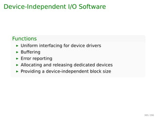
Other Issues — Program Structure
Example
▶ int[i][j] = int[128][128]
▶ Assuming page size is 128 words, then
▶ Each row (128 words) takes one page
If the process has fewer than 128 frames
Program 1:
for(j=0;j128;j++)
for(i=0;i128;i++)
data[i][j] = 0;
Worst case:
128 × 128 = 16, 384 page faults
Program 2:
for(i=0;i128;i++)
for(j=0;j128;j++)
data[i][j] = 0;
Worst case:
128 page faults
254 / 397

Other Issues — I/O interlock
Sometimes it is necessary to lock pages in memory so that
they are not paged out.
Example
▶ The OS
▶ I/O operation — the frame into which the I/O device was
scheduled to write should not be replaced.
▶ New page that was just brought in — looks like the best
candidate to be replaced because it was not accessed
yet, nor was it modiﬁed.
255 / 397

Case 1
Be sure the following sequence of events does not
occur:
1. A process issues an I/O request, and then queueing for
that I/O device
2. The CPU is given to other processes
3. These processes cause page faults
4. The waiting process’ page is unluckily replaced
5. When its I/O request is served, the speciﬁc frame is now
being used by another process
256 / 397

Case 2
Another bad sequence of events:
1. A low-priority process faults
2. The paging system selects a replacement frame. Then,
the necessary page is loaded into memory
3. The low-priority process is now ready to continue, and
waiting in the ready queue
4. A high-priority process faults
5. The paging system looks for a replacement
5.1 It sees a page that is in memory but not been referenced
nor modiﬁed: perfect!
5.2 It doesn’t know the page is just brought in for the
low-priority process
257 / 397

User’s View
▶ A program is a collection of segments
▶ A segment is a logical unit such as:
main program procedure function
method object local variables
global variables common block stack
symbol table arrays
259 / 397

Logical And Physical View of SegmentationLogical View of Segmentation
1
3
2
4
1
4
2
3
user space physical memory space
«
260 / 397

Segmentation Architecture
▶ Logical address consists of a two tuple:
segment-number, offset
▶ Segment table maps 2D virtual addresses into 1D
physical addresses; each table entry has:
▶ base contains the starting physical address where the
segments reside in memory
▶ limit speciﬁes the length of the segment
▶ Segment-table base register (STBR) points to the
segment table’s location in memory
▶ Segment-table length register (STLR) indicates number
of segments used by a program;
segment number s is legal if s STLR
261 / 397

Segmentation hardwareChapter 7 Main Memory
CPU
physical memory
s d
+
trap: addressing error
no
yes
segment
table
limit base
s
Figure 7.19 Segmentation hardware. 262 / 397

logical address space
subroutine stack
symbol
table
main
program
Sqrt
1400
physical memory
2400
3200
segment 2
4300
4700
5700
6300
6700
segment table
limit
0
1
2
3
4
1000
400
400
1100
1000
base
1400
6300
4300
3200
4700
segment 0
segment 3
segment 4
segment 2segment 1
segment 0
segment 3
segment 4
segment 1
(0, 1222) ⇒ Trap!
(3, 852) ⇒ 3200 + 852 = 4052
(2, 53) ⇒ 4300 + 53 = 4353
263 / 397

Advantages of Segmentation
▶ Each segment can be
▶ located independently
▶ separately protected
▶ grow independently
▶ Segments can be shared between processes
Problems with Segmentation
▶ Variable allocation
▶ Difficult to find holes in physical memory
▶ Must use one of non-trivial placement algorithm
▶ first fit, best fit, worst fit
▶ External fragmentation
264 / 397

Linux prefers paging to segmentation
Because
▶ Segmentation and paging are somewhat redundant
▶ Memory management is simpler when all processes
share the same set of linear addresses
▶ Maximum portability. RISC architectures in particular
have limited support for segmentation
The Linux 2.6 uses segmentation only when required by the
80x86 architecture.
265 / 397

Case Study: The Intel Pentium
Segmentation With Paging
|--------------- MMU ---------------|
+--------------+ +--------+ +----------+
+-----+ Logical | Segmentation | Linear | Paging | Physical | Physical |
| CPU |----------| unit |----------| unit |-----------| memory |
+-----+ address +--------------+ address +--------+ address +----------+
selector | offset
+----+---+---+--------+
| s | g | p | |
+----+---+---+--------+
13 1 2 32
+----------+----------+------------+
| p1 | p2 | d |
+----------+----------+------------+
10 10 12
| |
266 / 397

Segmentation
Logical Address ⇒ Linear Address7.7 Example: The Intel Pentium 309
logical address selector
descriptor table
segment descriptor +
32-bit linear address
offset
Figure 7.22 Intel Pentium segmentation.
268 / 397

Segment Selectors
A logical address consists of two parts:
segment selector : oﬀset
16 bits 32 bits
Segment selector is an index into GDT/LDT
selector | offset
+-----+-+--+--------+ s - segment number
| s |g|p | | g - 0-global; 1-local
+-----+-+--+--------+ p - protection use
13 1 2 32
269 / 397

Segment Descriptor Tables
All the segments are organized in 2 tables:
GDT Global Descriptor Table
▶ shared by all processes
▶ GDTR stores address and size of the GDT
LDT Local Descriptor Table
▶ one process each
▶ LDTR stores address and size of the LDT
Segment descriptors are entries in either GDT or LDT, 8-byte
long
Analogy
Process ⇐⇒ Process Descriptor(PCB)
File ⇐⇒ Inode
Segment ⇐⇒ Segment Descriptor
270 / 397

Segment Registers
The Intel Pentium has
▶ 6 segment registers, allowing 6 segments to be
addressed at any one time by a process
▶ Each segment register

an entry in LDT/GDT
▶ 6 8-byte micro program registers to hold descriptors
from either LDT or GDT
▶ avoid having to read the descriptor from memory for every
memory reference
0 1 2 3~8 9
+--------+--------|--------+---//---+--------+
| Segment selector| Micro program register |
+--------+--------|--------+---//---+--------+
Programmable Non-programmable
271 / 397

Fast access to segment descriptors
An additional nonprogrammable register for each
segment register
DESCRIPTOR TABLE SEGMENT
+--------------+ +------+
| ... | ,-------| |--.
+--------------+ | | | |
.---| Segment |____/ | | |
| | Descriptor | +------+ |
| +--------------+ |
| | ... | |
| +--------------+ |
| Nonprogrammable |
| Segment Registor Register |
__+------------------+--------------------+____/
| Segment Selector | Segment Descriptor |
+------------------+--------------------+
272 / 397

Segment registers hold segment selectors
cs code segment register
CPL 2-bit, speciﬁes the Current Privilege Level of
the CPU
00 - Kernel mode
11 - User mode
ss stack segment register
ds data segment register
es/fs/gs general purpose registers, may refer to arbitrary
data segments
273 / 397

Example: A LDT entry for code segment
Relative
address
0
4
Base 0-15 Limit 0-15
Base 24-31 Base 16-23
Limit
16-19
G D 0 P DPL Type
0: Li is in bytes
1: Li is in pages
Segment type and protection
S
;;
0: System
1: Application
32 Bits
Fig. 4-44. Pentium code segment descriptor. Data segments differ
slightly.
Base: Where the segment starts
Limit: 20 bit, ⇒ 220
in size
G: Granularity flag
0 - segment size in bytes
1 - in 4096 bytes
S: System flag
0 - system segment, e.g.
LDT
1 - normal code/data
segment
D/B: 0 - 16-bit offset
1 - 32-bit offset
Type: segment type (cs/ds/tss)
TSS: Task status, i.e. it’s
executing or not
DPL: Descriptor Privilege Level. 0
or 3
P: Segment-Present flag
0 - not in memory
1 - in memory
AVL: ignored by Linux
274 / 397

The Four Main Linux Segments
Every process in Linux has these 4 segments
Segment Base G Limit S Type DPL D/B P
user code 0x00000000 1 0xfffff 1 10 3 1 1
user data 0x00000000 1 0xfffff 1 2 3 1 1
kernel code 0x00000000 1 0xfffff 1 10 0 1 1
kernel data 0x00000000 1 0xfffff 1 2 0 1 1
All linear addresses start at 0, end at 4G-1
▶ All processes share the same set of linear addresses
▶ Logical addresses coincide with linear addresses
275 / 397

Pentium Paging
Linear Address ⇒ Physical Address
Two page size in Pentium:
4K:
2-level paging (Fig. 219)
4M:
1-level paging (Fig. 214)
+----------+----------+------------+
| p1 | p2 | d |
+----------+----------+------------+
10 10 12
| |
indicates that the size of the page frame is 4 MB and not the stan
If this ﬂag is set, the page directory points directly to the 4-MB p
bypassing the inner page table; and the 22 low-order bits in the line
refer to the offset in the 4-MB page frame.
page directory
page directory
CR3
register
page
directory
page
table
4-KB
page
4-MB
page
page table
offset
offset
(linear address)
31 22 21 12 11 0
2131 22 0
Figure 7.23 Paging in the Pentium architecture.
276 / 397

Paging In Linux
4-level paging for both 32-bit and 64-bit
Global directory Upper directory Middle directory Page Offset
Page
Page table
Page middle
directory
Page upper
directory
Page global
directory
Virtual
address
cr3
277 / 397

4-level paging for both 32-bit and 64-bit
▶ 64-bit: four-level paging
1. Page Global Directory
2. Page Upper Directory
3. Page Middle Directory
4. Page Table
▶ 32-bit: two-level paging
1. Page Global Directory
2. Page Upper Directory — 0 bits; 1 entry
3. Page Middle Directory — 0 bits; 1 entry
4. Page Table
The same code can work on 32-bit and 64-bit architectures
Page Address Paging Address
Arch size bits levels splitting
x86 4KB(12bits) 32 2 10 + 0 + 0 + 10 + 12
x86-PAE 4KB(12bits) 32 3 2 + 0 + 9 + 9 + 12
x86-64 4KB(12bits) 48 4 9 + 9 + 9 + 9 + 12
278 / 397

References
Wikipedia. Memory management — Wikipedia, The Free
2015.
Wikipedia. Virtual memory — Wikipedia, The Free
2015.
279 / 397

File Systems
Wang Xiaolin
April 9, 2016
280 / 397

Long-term Information Storage Requirements
▶ Must store large amounts of data
▶ Information stored must survive the termination of the
process using it
▶ Multiple processes must be able to access the
information concurrently
281 / 397

File-System Structure
File-system design addressing two problems:
1. defining how the FS should look to the user
▶ defining a file and its attributes
▶ the operations allowed on a file
▶ directory structure
2. creating algorithms and data structures to map the
logical FS onto the physical disk
282 / 397

File-System — A Layered Design
APPs
⇓
Logical FS
⇓
File-org module
⇓
Basic FS
⇓
I/O ctrl
⇓
Devices
▶ logical file system — manages metadata
information
- maintains all of the file-system structure
(directory structure, FCB)
- responsible for protection and security
▶ file-organization module
- logical block
address
translate
−−−−−→ physical block
address
- keeps track of free blocks
▶ basic file system issues generic
commands to device driver, e.g
- “read drive 1, cylinder 72, track 2,
sector 10”
▶ I/O Control — device drivers, and INT
handlers
- device driver:
high-level
commands
translate
−−−−−→ hardware-specific
instructions
283 / 397

The Operating Structure
APPs
⇓
Logical FS
⇓
File-org module
⇓
Basic FS
⇓
I/O ctrl
⇓
Devices
Example — To create a file
1. APP calls creat()
2. Logical FS
2.1 allocates a new FCB
2.2 updates the in-mem dir structure
2.3 writes it back to disk
2.4 calls the file-org module
3. file-organization module
3.1 allocates blocks for storing the file’s
data
3.2 maps the directory I/O into disk-block
numbers
Benefit of layered design
The I/O control and sometimes the basic file system code can
be used by multiple file systems.
284 / 397

File
A Logical View Of Information Storage
User’s view
A file is the smallest storage unit on disk.
▶ Data cannot be written to disk unless they are within a file
UNIX view
Each file is a sequence of 8-bit bytes
▶ It’s up to the application program to interpret this byte
stream.
285 / 397

File
What Is Stored In A File?
Source code, object files, executable files, shell scripts,
PostScript...
Different type of files have different structure
▶ UNIX looks at contents to determine type
Shell scripts start with “#!”
PDF start with “%PDF...”
Executables start with magic number
▶ Windows uses file naming conventions
executables end with “.exe” and “.com”
MS-Word end with “.doc”
MS-Excel end with “.xls”
286 / 397

File Naming
Vary from system to system
▶ Name length?
▶ Characters? Digits? Special characters?
▶ Extension?
▶ Case sensitive?
287 / 397

File Types
Regular files: ASCII, binary
Directories: Maintaining the structure of the FS
In UNIX, everything is a file
Character special files: I/O related, such as terminals,
printers ...
Block special files: Devices that can contain file systems, i.e.
disks
disks — logically, linear collections of
blocks; disk driver translates them
into physical block addresses
288 / 397

Binary ﬁles
(a) (b)
Header
Header
Header
Magic number
Text size
Data size
BSS size
Symbol table size
Entry point
Flags
Text
Data
Relocation
bits
Symbol
table
Object
module
Object
module
Object
module
Module
name
Date
Owner
Protection
Size
;
;;
Header
An UNIX executable ﬁle An UNIX archive
289 / 397

File Attributes — Metadata
▶ Name only information kept in human-readable form
▶ Identifier unique tag (number) identifies file within file
system
▶ Type needed for systems that support different types
▶ Location pointer to file location on device
▶ Size current file size
▶ Protection controls who can do reading, writing,
executing
▶ Time, date, and user identification data for protection,
security, and usage monitoring
290 / 397

File Operations
POSIX ﬁle system calls
1. fd = creat(name, mode)
2. fd = open(name, flags)
3. status = close(fd)
4. byte_count = read(fd, buffer, byte_count)
5. byte_count = write(fd, buffer, byte_count)
6. offset = lseek(fd, offset, whence)
7. status = link(oldname, newname)
8. status = unlink(name)
9. status = truncate(name, size)
10. status = ftruncate(fd, size)
11. status = stat(name, buffer)
12. status = fstat(fd, buffer)
13. status = utimes(name, times)
14. status = chown(name, owner, group)
15. status = fchown(fd, owner, group)
16. status = chmod(name, mode)
17. status = fchmod(fd, mode)
291 / 397

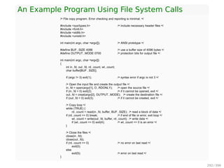
An Example Program Using File System Calls
/* File copy program. Error checking and reporting is minimal. */
#include sys/types.h /* include necessary header files */
#include fcntl.h
#include stdlib.h
#include unistd.h
int main(int argc, char *argv[]); /* ANSI prototype */
#define BUF SIZE 4096 /* use a buffer size of 4096 bytes */
#define OUTPUT MODE 0700 /* protection bits for output file */
int main(int argc, char *argv[])
{
int in fd, out fd, rd count, wt count;
char buffer[BUF SIZE];
if (argc != 3) exit(1); /* syntax error if argc is not 3 */
/* Open the input file and create the output file */
in fd = open(argv[1], O RDONLY); /* open the source file */
if (in fd 0) exit(2); /* if it cannot be opened, exit */
out fd = creat(argv[2], OUTPUT MODE); /* create the destination file */
if (out fd 0) exit(3); /* if it cannot be created, exit */
/* Copy loop */
while (TRUE) {
rd count = read(in fd, buffer, BUF SIZE); /* read a block of data */
if (rd count = 0) break; /* if end of file or error, exit loop */
wt count = write(out fd, buffer, rd count); /* write data */
if (wt count = 0) exit(4); /* wt count = 0 is an error */
}
/* Close the files */
close(in fd);
close(out fd);
if (rd count == 0) /* no error on last read */
exit(0);
else
exit(5); /* error on last read */
}
292 / 397

open()
fd open(pathname, flags)
A per-process open-file table is kept in the OS
▶ upon a successful open() syscall, a new entry is added into
this table
▶ indexed by file descriptor (fd)
To see files opened by a process, e.g. init
$ lsof -p 1
Why open() is needed?
To avoid constant searching
▶ Without open(), every file operation involves searching
the directory for the file.
293 / 397

Directories
Single-Level Directory Systems
All files are contained in the same directory
Root directory
A A B C
Fig. 6-7. A single-level directory system containing four files,
owned by three different people, A, B, and C.
- contains 4 files
- owned by 3 different
people, A, B, and C
Limitations
- name collision
- file searching
Often used on simple embedded devices, such as telephone,
digital cameras...
294 / 397

Directories
Two-level Directory Systems
A separate directory for each user
Files
User
directory
A A
A B
B
C
CC C
Root directory
Fig. 6-8. A two-level directory system. The letters indicate the
owners of the directories and files.
Limitation: hard to access others ﬁles
295 / 397

Directories
Hierarchical Directory Systems
User
directory
User subdirectories
C C
C
C C
C
B
B
A
A
B
B
C C
C
B
Root directory
User file
Fig. 6-9. A hierarchical directory system. 296 / 397

Directories
Path Names
ROOT
bin boot dev etc home var
grub passwd staff stud mail
w x 6 7 2 20081152001
dir
file
20081152001
297 / 397

Directories
Directory Operations
Create Delete Rename Link
Opendir Closedir Readdir Unlink
298 / 397

File System Implementation
A typical ﬁle system layout
|---------------------- Entire disk ------------------------|
+-----+-------------+-------------+-------------+-------------+
| MBR | Partition 1 | Partition 2 | Partition 3 | Partition 4 |
+-----+-------------+-------------+-------------+-------------+
_______________________________/ ____________
/
+---------------+-----------------+--------------------+---//--+
| Boot Ctrl Blk | Volume Ctrl Blk | Dir Structure | Files |
| (MBR copy) | (Super Blk) | (inodes, root dir) | dirs |
+---------------+-----------------+--------------------+---//--+
|-------------Master Boot Record (512 Bytes)------------|
0 439 443 445 509 511
+----//-----+----------+------+------//---------+---------+
| code area | disk-sig | null | partition table | MBR-sig |
| 440 | 4 | 2 | 16x4=64 | 0xAA55 |
+----//-----+----------+------+------//---------+---------+
299 / 397

On-Disk Information Structure
Boot control block a MBR copy
UFS: Boot block
NTFS: Partition boot sector
Volume control block Contains volume details
number of blocks size of blocks
free-block count free-block pointers
free FCB count free FCB pointers
UFS: Superblock
NTFS: Master File Table
Directory structure Organizes the files FCB, File control
block, contains file details (metadata).
UFS: I-node
NTFS: Stored in MFT using a relatiional database
structure, with one row per file
300 / 397

Each File-System Has a Superblock
Superblock
Keeps information about the ﬁle system
▶ Type — ext2, ext3, ext4...
▶ Size
▶ Status — how it’s mounted, free blocks, free inodes, ...
▶ Information about other metadata structures
# dumpe2fs /dev/sda1 | grep -i superblock
301 / 397

Implementing Files
Contiguous Allocation
also easy to retrieve a single block. For example, if a file starts at block b, and the ith
block of the file is wanted, its location on secondary storage is simply b ϩ i Ϫ 1. Con-
tiguous allocation presents some problems. External fragmentation will occur, mak-
ing it difficult to find contiguous blocks of space of sufficient length. From time to
time, it will be necessary to perform a compaction algorithm to free up additional
0 1 2 3 4
5 6 7
File A
File Allocation Table
File B
File C
File E
File D
8 9
10 11 12 13 14
15 16 17 18 19
20 21 22 23 24
25 26 27 28 29
30 31 32 33 34
File Name
File A
File B
File C
File D
File E
2
9
18
30
26
3
5
8
2
3
Start Block Length
Figure 12.7 Contiguous File Allocation
- simple;
- good for read only;
- fragmentation
302 / 397

Linked List (Chained) Allocation A pointer in each disk block
just a single entry for each file, showing the starting block and the length of the file.
Although preallocation is possible, it is more common simply to allocate blocks as
needed.The selection of blocks is now a simple matter: any free block can be added
to a chain. There is no external fragmentation to worry about because only one
Figure 12.9 Chained Allocation
0 1 2 3 4
5 6 7
File B
8 9
10 11 12 13 14
15 16 17 18 19
20 21 22 23 24
25 26 27 28 29
30 31 32 33 34
File B
File Name Start Block Length
1 5
- no waste
block;
- slow random
access;
- not 2n
303 / 397

Linked List (Chained) Allocation Though there is no external
fragmentation, consolidation is still preferred.574 CHAPTER 12 / FILE MANAGEMENT
block at a time is needed.This type of physical organization is best suited to sequen-
tial files that are to be processed sequentially. To select an individual block of a file
requires tracing through the chain to the desired block.
0 1 2 3 4
5 6 7
File B
8 9
10 11 12 13 14
15 16 17 18 19
20 21 22 23 24
25 26 27 28 29
30 31 32 33 34
File B
File Name Start Block Length
0 5
Figure 12.10 Chained Allocation (After Consolidation)
304 / 397

FAT: Linked list allocation with a table in RAM
▶ Taking the pointer out of each
disk block, and putting it into a
table in memory
▶ fast random access (chain is in
RAM)
▶ is 2n
▶ the entire table must be in RAM
disk ↗⇒ FAT ↗⇒ RAMused ↗
Physical
block
File A starts here
File B starts here
Unused block
0
1
2
3
4
5
6
7
8
9
10
11
12
13
14
15
10
11
7
3
2
12
14
-1
-1
Fig. 6-14. Linked list allocation using a file allocation table in
main memory.
305 / 397

Indexed Allocation 12.6 / SECONDARY STORAGE MANAGEMENT 575
Bit Tables This method uses a vector containing one bit for each block on the
disk. Each entry of a 0 corresponds to a free block, and each 1 corresponds to a
block in use. For example, for the disk layout of Figure 12.7, a vector of length 35 is
needed and would have the following value:
00111000011111000011111111111011000
Figure 12.11 Indexed Allocation with Block Portions
0 1 2 3 4
5 6 7
File B
8 9
10 11 12 13 14
15 16 17 18 19
20 21 22 23 24
25 26 27 28 29
30 31 32 33 34
File B
File Name Index Block
24
1
8
3
14
28
I-node A data structure for each ﬁle. An i-node is in
memory only if the ﬁle is open
filesopened ↗ ⇒ RAMused ↗
306 / 397

I-node — FCB in UNIX
File inode (128B)
Type Mode
User ID Group ID
File size # blocks
# links Flags
Timestamps (×3)
Triple indirect
Double indirect
Single indirect
Direct blocks (×12)
k #s of
ctory
ks
File data block
Data
File type Description
0 Unknown
1 Regular ﬁle
2 Directory
3 Character device
4 Block device
5 Named pipe
6 Socket
7 Symbolic link
Mode: 9-bit pattern
307 / 397

Inode Quiz
Given:
block size is 1KB
pointer size is 4B
Addressing:
byte oﬀset 9000
byte oﬀset 350,000
+----------------+
0 | 4096 |
+----------------+ ----+----------+ Byte 9000 in a file
1 | 228 | / | 367 | |
+----------------+ / | Data blk | v
2 | 45423 | / +----------+ 8th blk, 808th byte
+----------------+ /
3 | 0 | / --+------+
+----------------+ / / 0| |
4 | 0 | / / +------+
+----------------+ / / : : :
5 | 11111 | / / +------+ Byte 350,000
+----------------+ / -+-----+/ 75| 3333 | in a file
6 | 0 | / / 0| 331 | +------+ |
+----------------+ / / +-----+ : : : v
7 | 101 | / / | | +------+ 816th byte
+----------------+/ / | : | 255| | --+----------+
8 | 367 | / | : | +------+ | 3333 |
+----------------+ / | : | 331 | Data blk |
9 | 0 | / | | Single indirect +----------+
+----------------+ / +-----+
S | 428 (10K+256K) | / 255| |
+----------------+/ +-----+
D | 9156 | 9156 /***********************
+----------------+ Double indirect What about the ZEROs?
T | 824 | ***********************/
+----------------+
308 / 397

UNIX In-Core Data Structure
mount table — Info about each mounted FS
directory-structure cache — Dir-info of recently accessed dirs
inode table — An in-core version of the on-disk inode table
file table
▶ global
▶ keeps inode of each open file
▶ keeps track of
▶ how many processes are associated with
each open file
▶ where the next read and write will start
▶ access rights
user file descriptor table
▶ per process
▶ identifies all open files for a process
309 / 397

UNIX In-Core Data Structure
User
File Descriptor
Table
File
Table
Inode
Table
open()/creat()
1. add entry in each table
2. returns a ﬁle descriptor — an index into the user ﬁle
descriptor table
310 / 397

The Tables
Two levels of internal tables in the OS
A per-process table tracks all files that a process has open.
Stores
▶ the current-file-position pointer (not really)
▶ access rights
▶ more...
a.k.a file descriptor table
A system-wide table keeps process-independent
information, such as
▶ the location of the file on disk
▶ access dates
▶ file size
▶ file open count — the number of processes
opening this file
311 / 397

Per-process FDT
Process 1
+------------------+ System-wide
| ... | open-file table
+------------------+ +------------------+
| Position pointer | | ... |
| Access rights | +------------------+
| ... | | ... |
+------------------+ +------------------+
| ... | ---------| Location on disk |
+------------------+ | R/W |
| Access dates |
Process 2 | File size |
+------------------+ | Pointer to inode |
| Position pointer | | File-open count |
| Access rights |-----------| ... |
| ... | +------------------+
+------------------+ | ... |
| ... | +------------------+
+------------------+
312 / 397

A process executes the following code:
fd1 = open(/etc/passwd, O_RDONLY);
fd2 = open(local, O_RDWR);
fd3 = open(/etc/passwd, O_WRONLY);
STDIN
STDOUT
STDERR
...
User
File descriptor
table
0
1
2
3
4
5
...
...
count 1
R
...
count 1
RW
...
count 1
W
Global
open ﬁle
table
...
...
...
(/etc/passwd)
count 2
...
(local)
count 1
...
Inode table
313 / 397

One more process B:
fd1 = open(/etc/passwd, O_RDONLY);
fd2 = open(private, O_RDONLY);
STDIN
STDOUT
STDERR
...
Proc B
User
File descriptor
table
0
1
2
3
4
5
...
...
count 1
R
...
count 1
RW
...
count 1
R
...
count 1
W
...
count 1
R
Global
open ﬁle
table
...
...
(/etc/passwd)
count 3
...
...
(local)
count 1
...
...
(private)
count 1
...
...
Inode table
STDIN
STDOUT
STDERR
...
Proc B
0
1
2
3
4
...
314 / 397

Why File Table?
To allow a parent and child to share a ﬁle position, but to
provide unrelated processes with their own values.
Mode
i-node
Link count
Uid
Gid
File size
Times
Addresses of
first 10
disk blocks
Single indirect
Double indirect
Triple indirect
Parent’s
file
descriptor
table
Child’s
file
descriptor
table
Unrelated
process
file
descriptor
table
Open file
description
File position
R/W
Pointer to i-node
File position
R/W
Pointer to i-node
P
di‘
315 / 397

Why File Table?
Where To Put File Position Info?
Inode table? No. Multiple processes can open the same file.
Each one has its own file position.
User file descriptor table? No. Trouble in file sharing.
Example
#!/bin/bash
echo hello
echo world
Where should the “world” be?
$ ./hello.sh A
316 / 397

Implementing Directories
(a)
games
mail
news
work
attributes
attributes
attributes
attributes
Data structure
containing the
attributes
(b)
games
mail
news
work
Fig. 6-16. (a) A simple directory containing fixed-size entries with
the disk addresses and attributes in the directory entry. (b) A direc-
tory in which each entry just refers to an i-node.
(a) A simple directory (Windows)
▶ ﬁxed size entries
▶ disk addresses and attributes in directory entry
(b) Directory in which each entry just refers to an i-node
(UNIX)
317 / 397

How Long A File Name Can Be?
File 1 entry length
File 1 attributes
Pointer to file 1's name
File 1 attributes
File 2 attributes
File 2 entry length
File 2 attributes
File 3 entry length
File 3 attributes
p
e
b
e
r
c
u
t
o
t
d
j
-
g
p
e
b
e
r
c
u
t
o
t
d
j
-
g
p
e r s o
n n e l
f o o
p
o
l
e
n
r
n
f o o
s
e
Entry
for one
file
Heap
Entry
for one
file
(a) (b)
File 3 attributes
318 / 397

UNIX Treats a Directory as a File
Directory inode (128B)
Type Mode
User ID Group ID
File size # blocks
# links Flags
Timestamps (×3)
Triple indirect
Double indirect
Single indirect
.
..
passwd
fstab
… …
Directory block
File inode (128B)
Type Mode
User ID Group ID
File size # blocks
# links Flags
Timestamps (×3)
Triple indirect
Double indirect
Single indirect
Indirect block
inode #
inode #
inode #
inode #
Block #s of
more
directory
blocks
Block # of
block with
512 single
indirect
entries
Block # of
block with
512 double
indirect
entries
File data block
Data
Example
. 2
.. 2
bin 11116545
boot 2
cdrom 12
dev 3
.
.
.
.
.
.
319 / 397

The steps in looking up /usr/ast/mbox
Root directory
I-node 6
is for /usr
Block 132
is /usr
directory
I-node 26
is for
/usr/ast
Block 406
is /usr/ast
directory
Looking up
usr yields
i-node 6
I-node 6
says that
/usr is in
block 132
/usr/ast
is i-node
26
/usr/ast/mbox
is i-node
60
I-node 26
says that
/usr/ast is in
block 406
1
1
4
7
14
9
6
8
.
..
bin
dev
lib
etc
usr
tmp
6
1
19
30
51
26
45
dick
erik
jim
ast
bal
26
6
64
92
60
81
17
grants
books
mbox
minix
src
Mode
size
times
132
Mode
size
times
406
320 / 397

File Sharing
Multiple Users
User IDs identify users, allowing permissions and
protections to be per-user
Group IDs allow users to be in groups, permitting group
access rights
Example: 9-bit pattern
rwxr-x--- means:
user group other
rwx r-x ---
111 1-1 000
7 5 0
321 / 397

File Sharing
Remote File Systems
Networking — allows file system access between
systems
▶ Manually via programs like FTP
▶ Automatically, seamlessly using distributed file systems
▶ Semi automatically, via the world wide web
C/S model — allows clients to mount remote file systems
from servers
▶ NFS — standard UNIX client-server file sharing protocol
▶ CIFS — standard Windows protocol
▶ Standard system calls are translated into remote calls
Distributed Information Systems (distributed naming
services)
▶ such as LDAP, DNS, NIS, Active Directory implement
unified access to information needed for remote computing
322 / 397

File Sharing
Protection
▶ File owner/creator should be able to control:
▶ what can be done
▶ by whom
▶ Types of access
▶ Read
▶ Write
▶ Execute
▶ Append
▶ Delete
▶ List
323 / 397

Shared Files
Hard Links vs. Soft Links
Root directory
B
B B C
C C
CA
B C
B
? C C C
A
Shared file
Fig. 6-18. File system containing a shared file. 324 / 397

Drawback
C's directory B's directory B's directoryC's directory
Owner = C
Count = 1
Owner = C
Count = 2
Owner = C
Count = 1
(a) (b) (c)
326 / 397

Symbolic Links
A symbolic link has its own inode

Disk Space Management
Statistics
328 / 397

▶ Block size is chosen while creating the FS
▶ Disk I/O performance is conﬂict with space utilization
▶ smaller block size ⇒ better space utilization
▶ larger block size ⇒ better disk I/O performance
$ dumpe2fs /dev/sda1 | grep Block size
329 / 397

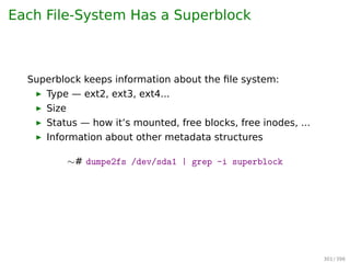
Keeping Track of Free Blocks
1. Linked List10.5 Free-Space Management 443
0 1 2 3
4 5 7
8 9 10 11
12 13 14
16 17 18 19
20 21 22 23
24 25 26 27
28 29 30 31
15
6
st head
10 Linked free-space list on disk.
2. Bit map (n blocks)
0 1 2 3 4 5 6 7 8 .. n-1
+-+-+-+-+-+-+-+-+-+-//-+-+
|0|0|1|0|1|1|1|0|1| .. |0|
+-+-+-+-+-+-+-+-+-+-//-+-+
bit[i] =
{
0 ⇒ block[i] is free
1 ⇒ block[i] is occupied
330 / 397

Journaling File Systems
Operations required to remove a ﬁle in UNIX:
1. Remove the ﬁle from its directory
- set inode number to 0
2. Release the i-node to the pool of free i-nodes
- clear the bit in inode bitmap
3. Return all the disk blocks to the pool of free disk blocks
- clear the bits in block bitmap
What if crash occurs between 1 and 2, or between 2 and 3?
331 / 397

Journaling File Systems
Keep a log of what the ﬁle system is going to do
before it does it
▶ so that if the system crashes before it can do its planned
work, upon rebooting the system can look in the log to
see what was going on at the time of the crash and ﬁnish
the job.
▶ NTFS, EXT3, and ReiserFS use journaling among others
332 / 397

Ext2 Block groups
The partition is divided into Block Groups
▶ Block groups are same size — easy locating
▶ Kernel tries to keep a ﬁle’s data blocks in the same block
group — reduce fragmentation
▶ Backup critical info in each block group
▶ The Ext2 inodes for each block group are kept in the
inode table
▶ The inode-bitmap keeps track of allocated and
unallocated inodes
334 / 397

Group descriptor
▶ Each block group has a group descriptor
▶ All the group descriptors together make the group
descriptor table
▶ The table is stored along with the superblock
▶ Block Bitmap: tracks free blocks
▶ Inode Bitmap: tracks free inodes
▶ Inode Table: all inodes in this block group
▶
Free blocks count
Free Inodes count
Used dir count
}
counters
See more: # dumpe2fs /dev/sda1
335 / 397

Maths
Given
block size = 4K
block bitmap = 1 blk
, then
blocks per group = 8 bits × 4K = 32K
How large is a group?
group size = 32K × 4K = 128 M
How many block groups are there?
≈
partition size
group size
=
partition size
128M
How many ﬁles can I have in max?
≈
partition size
block size
=
partition size
4K
336 / 397

Ext2 Block Allocation PoliciesChapter 15 The Linux System
allocating scattered free blocks
allocating continuous free blocks
block in use bit boundary
block selected
by allocator
free block byte boundarybitmap search
Figure 15.9 ext2fs block-allocation policies.
337 / 397

Ext2 inode
Mode: holds two pieces of information
1. Is it a
{file|dir|sym-link|blk-dev|char-dev|FIFO}?
2. Permissions
Owner info: Owners’ ID of this file or directory
Size: The size of the file in bytes
Timestamps: Accessed, created, last modified time
Datablocks: 15 pointers to data blocks (12 + S + D + T)
339 / 397

Max File Size
Given: {
block size = 4K
pointer size = 4B
,
We get:
Max File Size = number of pointers × block size
= (
number of pointers
12
direct
+ 1K
1−indirect
+ 1K × 1K
2−indirect
+ 1K × 1K × 1K
3−indirect
) × 4K
= 48K + 4M + 4G + 4T
340 / 397

Ext2 Superblock
Magic Number: 0xEF53
Revision Level: determines what new features are available
Mount Count and Maximum Mount Count: determines if the
system should be fully checked
Block Group Number: indicates the block group holding this
superblock
Block Size: usually 4K
Blocks per Group: 8bits × block size
Free Blocks: System-wide free blocks
Free Inodes: System-wide free inodes
First Inode: First inode number in the ﬁle system
See more: ∼# dumpe2fs /dev/sda1
341 / 397

Ext2 File Types
File type Description
0 Unknown
1 Regular file
2 Directory
3 Character device
4 Block device
5 Named pipe
6 Socket
7 Symbolic link
Device file, pipe, and socket: No data blocks are required.
All info is stored in the inode
Fast symbolic link: Short path name ( 60 chars) needs no
data block. Can be stored in the 15 pointer fields
342 / 397

Ext2 Directories
0 11|12 23|24 39|40
+----+--+-+-+----+----+--+-+-+----+----+--+-+-+----+----+--//--+
| 21 |12|1|2|. | 22 |12|2|2|.. | 53 |16|5|2|hell|o | |
+----+--+-+-+----+----+--+-+-+----+----+--+-+-+----+----+--//--+
,-------- inode number
| ,--- record length
| | ,--- name length
| | | ,--- file type
| | | | ,---- name
+----+--+-+-+----+
0 | 21 |12|1|2|. |
+----+--+-+-+----+
12| 22 |12|2|2|.. |
+----+--+-+-+----+----+
24| 53 |16|5|2|hell|o |
+----+--+-+-+----+----+
40| 67 |28|3|2|usr |
+----+--+-+-+----+----+
52| 0 |16|7|1|oldf|ile |
+----+--+-+-+----+----+
68| 34 |12|4|2|sbin|
+----+--+-+-+----+
▶ Directories are special files
▶ “.” and “..” first
▶ Padding to 4 ×
▶ inode number is 0 — deleted
file
343 / 397

Many diﬀerent FS are in use
Windows
uses drive letter (C:, D:, ...) to identify each FS
UNIX
integrates multiple FS into a single structure
▶ From user’s view, there is only one FS hierarchy
$ man fs
344 / 397

$ cp /floppy/TEST /tmp/test
cp
VFS
ext2 MS-DOS
/tmp/test /ﬂoppy/TEST
1 inf = open(/floppy/TEST, O_RDONLY, 0);
2 outf = open(/tmp/test,
3 O_WRONLY|O_CREAT|O_TRUNC, 0600);
4 do {
5 i = read(inf, buf, 4096);
6 write(outf, buf, i);
7 } while (i);
8 close(outf);
9 close(inf);
345 / 397

ret = write(fd, buf, len);
of the filesystem implementation, to write the data to the media (or whatever this filesys-
tem does on write). Figure 13.2 shows the flow from user-space’s write() call through
the data arriving on the physical media. On one side of the system call is the genericVFS
interface, providing the frontend to user-space; on the other side of the system call is the
filesystem-specific backend, dealing with the implementation details.The rest of this chap-
ter looks at how theVFS achieves this abstraction and provides its interfaces.
Unix Filesystems
Historically, Unix has provided four basic filesystem-related abstractions: files, directory
entries, inodes, and mount points.
A filesystem is a hierarchical storage of data adhering to a specific structure. Filesystems
contain files, directories, and associated control information.Typical operations performed
user-space VFS filesystem physical media
write( ) sys_write( )
filesystem’s
write method
Figure 13.2 The flow of data from user-space issuing a write() call, through the
VFS’s generic system call, into the filesystem’s specific write method, and finally
arriving at the physical media.
346 / 397

Virtural File Systems
Put common parts of all FS in a separate layer
▶ It’s a layer in the kernel
▶ It’s a common interface to several kinds of ﬁle systems
▶ It calls the underlying concrete FS to actual manage the
data
User
process
FS 1 FS 2 FS 3
Buffer cache
Virtual file system
File
system
VFS interface
POSIX
347 / 397

Virtual File System
▶ Manages kernel level file abstractions in one format for
all file systems
▶ Receives system call requests from user level (e.g. write,
open, stat, link)
▶ Interacts with a specific file system based on mount
point traversal
▶ Receives requests from other parts of the kernel, mostly
from memory management
Real File Systems
▶ managing file directory data
▶ managing meta-data: timestamps, owners, protection,
etc.
▶ disk data, NFS data...
translate
←−−−−−→ VFS data
348 / 397

File System Mounting
/
a b a
c
p q r q q r
d
/
c d
b
Diskette
/
Hard diskHard disk
x y z
x y z
Fig. 10-26. (a) Separate file systems. (b) After mounting.
349 / 397

A FS must be mounted before it can be used
Mount — The ﬁle system is registered with the VFS
▶ The superblock is read into the VFS superblock
▶ The table of addresses of functions the VFS requires is
read into the VFS superblock
▶ The FS’ topology info is mapped onto the VFS superblock
data structure
The VFS keeps a list of the mounted ﬁle systems
together with their superblocks
The VFS superblock contains:
▶ Device, blocksize
▶ Pointer to the root inode
▶ Pointer to a set of superblock routines
▶ Pointer to file_system_type data structure
▶ more...
350 / 397

V-node
▶ Every ﬁle/directory in the VFS has a VFS inode, kept in
the VFS inode cache
▶ The real FS builds the VFS inode from its own info
Like the EXT2 inodes, the VFS inodes describe
▶ ﬁles and directories within the system
▶ the contents and topology of the Virtual File System
351 / 397

VFS Operation
read()
...
Process
table
0
File
descriptors
...
V-nodes
open
read
write
Function
pointers
...2
4
VFS
Read
function
FS 1
Call from
VFS into
FS 1
352 / 397

Linux VFS
The Common File Model
All other filesystems must map their own concepts into the
common file model
For example, FAT filesystems do not have inodes.
▶ The main components of the common file model are
superblock – information about mounted filesystem
inode – information about a specific file
file – information about an open file
dentry – information about directory entry
▶ Geared toward Unix FS
353 / 397

The Superblock Object
▶ is implemented by each FS and is used to store
information describing that specific FS
▶ usually corresponds to the filesystem superblock or the
filesystem control block
▶ Filesystems that are not disk-based (such as sysfs, proc)
generate the superblock on-the-fly and store it in
memory
▶ struct super_block in linux/fs.h
▶ s_op in struct super_block

struct super_operations —
the superblock operations table
▶ Each item in this table is a pointer to a function that
operates on a superblock object
354 / 397

The Inode Object
▶ For Unix-style filesystems, this information is simply read
from the on-disk inode
▶ For others, the inode object is constructed in memory in
whatever manner is applicable to the filesystem
▶ struct inode in linux/fs.h
▶ An inode represents each file on a FS, but the inode
object is constructed in memory only as files are
accessed
▶ includes special files, such as device files or pipes
▶ i_op

struct inode_operations
355 / 397

The Dentry Object
▶ components in a path
▶ makes path name lookup easier
▶ struct dentry in linux/dcache.h
▶ created on-the-ﬂy from a string representation of a path
name
356 / 397

Dentry State
▶ used
▶ unused
▶ negative
Dentry Cache
consists of three parts:
1. Lists of “used”dentries
2. A doubly linked “least recently used”list of unused and
negative dentry objects
3. A hash table and hashing function used to quickly
resolve a given path into the associated dentry object
357 / 397

The File Object
▶ is the in-memory representation of an open file
▶ open() ⇒ create; close() ⇒ destroy
▶ there can be multiple file objects in existence for the
same file
▶ Because multiple processes can open and manipulate a file
at the same time
▶ struct file in linux/fs.h
358 / 397

Process 1
Process 2
Process 3
File object
File object
File object
dentry
object
dentry
object
inode
object
Superblock
object
disk
ﬁle
fd f_dentry
d_inode
i_sb
359 / 397

References
Wikipedia. Computer ﬁle — Wikipedia, The Free
2015.
Wikipedia. Ext2 — Wikipedia, The Free Encyclopedia.
[Online; accessed 21-February-2015]. 2015.
Wikipedia. File system — Wikipedia, The Free
2015.
Wikipedia. Inode — Wikipedia, The Free Encyclopedia.
[Online; accessed 21-February-2015]. 2015.
Wikipedia. Virtual ﬁle system — Wikipedia, The Free
2014.
360 / 397

I/O Systems
Wang Xiaolin
April 9, 2016
u wx672ster@gmail.com
361 / 397

I/O Hardware
Diﬀerent people, diﬀerent view
▶ Electrical engineers: chips, wires, power supplies,
motors...
▶ Programmers: interface presented to the software
▶ the commands the hardware accepts
▶ the functions it carries out
▶ the errors that can be reported back
▶ ...
362 / 397

I/O Devices
Roughly two Categories:
1. Block devices: store information in ﬁx-size blocks
2. Character devices: deal with streams of characters
363 / 397

Device Controllers
I/O units usually consist of
1. a mechanical component
2. an electronic component is called the device controller
or adapter
e.g. video adapter, network adapter...
Monitor
Keyboard
Floppy
disk drive
Hard
disk drive
Hard
disk
controller
Floppy
disk
controller
Keyboard
controller
Video
controller
MemoryCPU
Bus
364 / 397

Port: A connection point. A device communicates with
the machine via a port — for example, a serial
port.
Bus: A set of wires and a rigidly deﬁned protocol that
speciﬁes a set of messages that can be sent on
the wires.
Controller: A collection of electronics that can operate a
port, a bus, or a device.
e.g. serial port controller, SCSI bus controller,
disk controller...
365 / 397

The Controller’s Job
Examples:
▶ Disk controllers: convert the serial bit stream into a block
of bytes and perform any error correction necessary
▶ Monitor controllers: read bytes containing the characters
to be displayed from memory and generates the signals
used to modulate the CRT beam to cause it to write on
the screen
366 / 397

Inside The Controllers
Control registers: for communicating with the CPU (R/W,
On/Off...)
Data buffer: for example, a video RAM
Q: How the CPU communicates with the control registers
and the device data buffers?
A: Usually two ways...
367 / 397

(a) Each control register is assigned an I/O port number,
then the CPU can do, for example,
▶ read in control register PORT and store the result in CPU
register REG.
IN REG, PORT
▶ write the contents of REG to a control register
OUT PORT, REG
Note: the address spaces for memory and I/O are
diﬀerent. For example,
▶ read the contents of I/O port 4 and puts it in R0
IN R0, 4 ; 4 is a port number
▶ read the contents of memory word 4 and puts it in R0
MOV R0, 4 ; 4 is a memory address
368 / 397

Address spaces
Two address One address space Two address spaces
Memory
I/O ports
0xFFFF…
0
(a) (b) (c)
Fig. 5-2. (a) Separate I/O and memory space. (b) Memory-mapped
I/O. (c) Hybrid.
(a) Separate I/O and memory space
(b) Memory-mapped I/O: map all the control registers into
the memory space. Each control register is assigned a
unique memory address.
(c) Hybrid: with memory-mapped I/O data buﬀers and
separate I/O ports for the control registers. For example,
Intel Pentium
▶ Memory addresses 640K to 1M being reserved for device
data buﬀers
▶ I/O ports 0 through 64K.
369 / 397

Advantages of Memory-mapped I/O
No assembly code is needed (IN, OUT...)
With memory-mapped I/O, device control registers are just
variables in memory and can be addressed in C the same
way as any other variables. Thus with memory-mapped I/O,
a I/O device driver can be written entirely in C.
No special protection mechanism is needed
The I/O address space is part of the kernel space, thus
cannot be touched directly by any user space process.
370 / 397

Disadvantages of Memory-mapped I/O
Caching problem
▶ Caching a device control register would be disastrous
▶ Selectively disabling caching adds extra complexity to
both hardware and the OS
Problem with multiple buses
CPU Memory I/O
Bus
All addresses (memory
and I/O) go here
CPU Memory I/O
CPU reads and writes of memory
go over this high-bandwidth bus
This memory port is
to allow I/O devices
access to memory
(a) (b)
Fig. 5-3. (a) A single-bus architecture. (b) A dual-bus memory
architecture.
Figure: (a) A single-bus architecture. (b) A dual-bus memory
architecture.
371 / 397

Programmed I/O
Handshaking
...........
busy = ?
.
0
.....
write a byte
.....
command-ready = 1
.....
command-ready = ?
.
1
.....
busy = 1
.....
write == 1?
.
1
.....
read
.
1 byte
.....
command-ready = 0, error = 0, busy = 0
.Host:. status:Register. control:Register. data-out:Register. Controller:
372 / 397

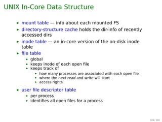
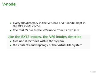
Example
Steps in printing a string
String to
be printedUser
space
Kernel
space
ABCD
EFGH
Printed
page
(a)
ABCD
EFGH
ABCD
EFGH
Printed
page
(b)
A
Next
(c)
AB
Next
Fig. 5-6. Steps in printing a string.
1 copy_from_user(buffer, p, count); /* p is the kernel bufer */
2 for (i = 0; i count; i++) { /* loop on every character */
3 while(*printer_status_reg != READY); /* loop until ready */
4 *printer_data_register = p[i]; /* output one character */
5 }
6 return_to_user();
373 / 397

Pulling Is Ineﬃcient
A better way
Interrupt The controller notiﬁes the CPU when the device
is ready for service.1.2 Computer-System Organization 9
user
process
executing
CPU
I/O interrupt
processing
I/O
request
transfer
done
I/O
request
transfer
done
I/O
device
idle
transferring
Figure 1.3 Interrupt time line for a single process doing output.
374 / 397

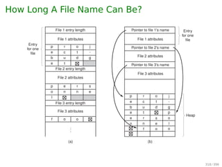
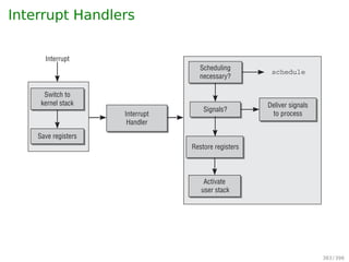
Example
Writing a string to the printer using interrupt-driven I/O
When the print system call is made...
1 copy_from_user(buffer, p, count);
2 enable_interrupts();
3 while(*printer_status_reg != READY);
4 *printer_data_register = p[0];
5 scheduler();
Interrupt service procedure for the printer
1 if (count == 0) {
2 unblock_user();
3 } else {
4 *printer_data_register = p[1];
5 count = count - 1;
6 i = i + 1;
7 }
8 acknowledge_interrupt();
9 return_from_interrupt();
375 / 397

Direct Memory Access (DMA)
Programmed I/O (PIO) tying up the CPU full time until all the
I/O is done (busy waiting)
Interrupt-Driven I/O an interrupt occurs on every charcater
(wastes CPU time)
Direct Memory Access (DMA) Uses a special-purpose
processor (DMA controller) to work with the I/O
controller
376 / 397

Example
Printing a string using DMA
In essence, DMA is programmed I/O, only with the DMA
controller doing all the work, instead of the main CPU.
When the print system call is made...
1 copy_from_user(buffer, p, count);
2 set_up_DMA_controller();
3 scheduler();
Interrupt service procedure
1 acknowledge_interrupt();
2 unblock_user();
3 return_from_interrupt();
The big win with DMA is reducing the number of interrupts
from one per character to one per buﬀer printed.
377 / 397

DMA Handshaking Example
Read from disk
..........
read
.
data
.....
data ready?
.
yes
.....
DMA-request
.......
DMA-acknowledge
...
memory address
.....
data
.Disk:. Disk Controller:. DMA Controller:. Memory:
378 / 397

The DMA controller
▶ has access to the system bus independent of the CPU
▶ contains several registers that can be written and read
by the CPU. These includes
▶ a memory address register
▶ a byte count register
▶ one or more control registers
▶ specify the I/O port to use
▶ the direction of the transfer (read/write)
▶ the transfer unit (byte/word)
▶ the number of bytes to transfer in one burst.
379 / 397

CPU
DMA
controller
Disk
controller
Main
memory
Buffer
1. CPU
programs
the DMA
controller
Interrupt when
done
2. DMA requests
transfer to memory 3. Data transferred
Bus
4. Ack
Address
Count
Control
Drive
Fig. 5-4. Operation of a DMA transfer.
380 / 397

I/O Software Layers
I/O
request
Layer
I/O
reply I/O functions
Make I/O call; format I/O; spooling
Naming, protection, blocking, buffering, allocation
Set up device registers; check status
Wake up driver when I/O completed
Perform I/O operation
User processes
Device-independent
software
Device drivers
Interrupt handlers
Hardware
Fig. 5-16. Layers of the I/O system and the main functions of each
layer.
381 / 397

Interrupt Handlers
oes not change when kernel code is executed. The platform-specific data structure pt_regs that lists a
egisters modified in kernel mode is defined to take account of the differences between the various CPU
Section 14.1.7 takes a closer look at this). Low-level routines coded in assembly language are responsib
or filling the structure.
Interrupt
Handler
Scheduling
necessary?
Signals?
Restore registers
Deliver signals
to process
Activate
user stack
Switch to
kernel stack
Save registers
Interrupt
schedule
Figure 14-2: Handling an interrupt.
n the exit path the kernel checks whether
❑ the scheduler should select a new process to replace the old process. 382 / 397

Device Drivers
User
space
Kernel
space
User process
User
program
Rest of the operating system
Printer
driver
Camcorder
driver
CD-ROM
driver
Printer controllerHardware
Devices
Camcorder controller CD-ROM controller
383 / 397

Device-Independent I/O Software
Functions
▶ Uniform interfacing for device drivers
▶ Buﬀering
▶ Error reporting
▶ Allocating and releasing dedicated devices
▶ Providing a device-independent block size
384 / 397

Uniform Interfacing for Device Drivers
Operating system Operating system
Disk driver Printer driver Keyboard driver Disk driver Printer driver Keyboard driver
(a) (b)
Fig. 5-13. (a) Without a standard driver interface. (b) With a stan-
dard driver interface.
385 / 397

Buﬀering
User process
User
space
Kernel
space
2 2
1 1 3
Modem Modem Modem Modem
(a) (b) (c) (d)
Fig. 5-14. (a) Unbuffered input. (b) Buffering in user space.
(c) Buffering in the kernel followed by copying to user space. (d)
Double buffering in the kernel.
386 / 397

User-Space I/O Software
Examples:
▶ stdio.h, printf(), scanf()...
▶ spooling(printing, USENET news...)
387 / 397

Disk
458 Chapter 11 Mass-Storage Structure
track t
sector s
spindle
cylinder c
platter
arm
read-write
head
arm assembly
rotation
Figure 11.1 Moving-head disk mechanism.
A read–write head “ﬂies” just above each surface of every platter. The388 / 397

Disk Scheduling
First Come First Serve (FCFS)
Chapter 11 Mass-Storage Structure
0 14 37 536567 98 122124 183199
queue ϭ 98, 183, 37, 122, 14, 124, 65, 67
head starts at 53
Figure 11.4 FCFS disk scheduling.
389 / 397

Disk Scheduling
Shortest Seek Time First (SSTF)
11.4 Disk Scheduling 46
0 14 37 536567 98 122124 183199
queue ϭ 98, 183, 37, 122, 14, 124, 65, 67
head starts at 53
Figure 11.5 SSTF disk scheduling.
390 / 397

Disk Scheduling
SCAN Scheduling
Chapter 11 Mass-Storage Structure
0 14 37 536567 98 122124 183199
queue ϭ 98, 183, 37, 122, 14, 124, 65, 67
head starts at 53
Figure 11.6 SCAN disk scheduling.
391 / 397

Disk Scheduling
Circular SCAN (C-SCAN) Scheduling
C-SCAN scheduling algorithm essentially treats the cylinders as a circular lis
hat wraps around from the ﬁnal cylinder to the ﬁrst one.
0 14 37 53 65 67 98 122124 183199
queue = 98, 183, 37, 122, 14, 124, 65, 67
head starts at 53
Figure 11.7 C-SCAN disk scheduling.
392 / 397

Operating Systems (slides)

More Related Content

What's hot

Similar to Operating Systems (slides)

Recently uploaded

Operating Systems (slides)