Operating System CPU Scheduling slide with OS

Silberschatz, Galvin and Gagne 2002
6.1
Operating System Concepts
Chapter 6: CPU Scheduling
 Basic Concepts
 Scheduling Criteria
 Scheduling Algorithms
 Multiple-Processor Scheduling
 Real-Time Scheduling
 Algorithm Evaluation

6.2
Basic Concepts
 Maximum CPU utilization obtained with
multiprogramming
 CPU–I/O Burst Cycle – Process execution consists of a
cycle of CPU execution and I/O wait.
 CPU burst distribution

6.3
Alternating Sequence of CPU And I/O
Bursts
 Process execution begins with a CPU
burst. That is followed by an IO
burst, then another CPU burst, then
another I/O burst, and so on.
 Eventually, the last CPU burst will
end with a system request to
terminate execution, rather than with
another I/O burst

6.4
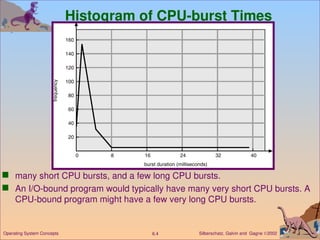
Histogram of CPU-burst Times
 many short CPU bursts, and a few long CPU bursts.
 An I/O-bound program would typically have many very short CPU bursts. A
CPU-bound program might have a few very long CPU bursts.

6.5
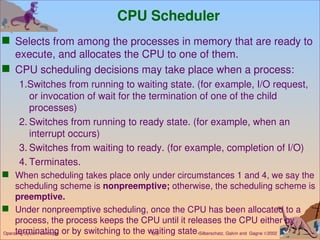
CPU Scheduler
 Selects from among the processes in memory that are ready to
execute, and allocates the CPU to one of them.
 CPU scheduling decisions may take place when a process:
1.Switches from running to waiting state. (for example, I/O request,
or invocation of wait for the termination of one of the child
processes)
2. Switches from running to ready state. (for example, when an
interrupt occurs)
3. Switches from waiting to ready. (for example, completion of I/O)
4. Terminates.
 When scheduling takes place only under circumstances 1 and 4, we say the
scheduling scheme is nonpreemptive; otherwise, the scheduling scheme is
preemptive.
 Under nonpreemptive scheduling, once the CPU has been allocated to a
process, the process keeps the CPU until it releases the CPU either by
terminating or by switching to the waiting state.

6.6
Dispatcher
 Dispatcher module gives control of the CPU to the process
selected by the short-term scheduler; this involves:
 switching context
 switching to user mode
 jumping to the proper location in the user program to restart that
program
 Dispatch latency – time it takes for the dispatcher to stop one
process and start another running.

6.7
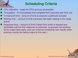
Scheduling Criteria
 CPU utilization – keep the CPU as busy as possible
 Throughput – # of processes that complete their execution per time unit
 Turnaround time – amount of time to execute a particular process
 Waiting time – amount of time a process has been waiting in the ready
queue
 Response time – amount of time it takes from when a request was
submitted until the first response is produced. (a process can produce
some output fairly early, and can continue computing new results while
previous results are being output to the user.)

6.8
Optimization Criteria
 Max CPU utilization
 Max throughput
 Min turnaround time
 Min waiting time
 Min response time

6.9
First-Come, First-Served (FCFS) Scheduling
Process Burst Time
P1 24
P2 3
P3 3
 Suppose that the processes arrive in the order: P1 , P2 , P3
The Gantt Chart for the schedule is:
 Waiting time for P1 = 0; P2 = 24; P3 = 27
 Average waiting time: (0 + 24 + 27)/3 = 17
P1 P2 P3
24 27 30
0

6.10
FCFS Scheduling (Cont.)
Suppose that the processes arrive in the order
P2 , P3 , P1 .
 The Gantt chart for the schedule is:
 Waiting time for P1 = 6; P2 = 0; P3 = 3
 Average waiting time: (6 + 0 + 3)/3 = 3
 Much better than previous case.
 The effect short process behind long process
P1
P3
P2
6
3 30
0

6.11
Shortest-Job-First (SJR) Scheduling
 Associate with each process the length of its next CPU burst.
Use these lengths to schedule the process with the shortest
time.
 Two schemes:
 nonpreemptive – once CPU given to the process it cannot be
preempted until completes its CPU burst.
 preemptive – if a new process arrives with CPU burst length less
than remaining time of current executing process, preempt. This
scheme is know as the
Shortest-Remaining-Time-First (SRTF).
 SJF is optimal – gives minimum average waiting time for a
given set of processes.

6.12
ProcessArrival Time Burst Time
P1 0.0 7
P2 2.0 4
P3 4.0 1
P4 5.0 4
 SJF (non-preemptive)
 Average waiting time = (0 + 6 + 3 + 7)/4 =4
Example of Non-Preemptive SJF
P1 P3 P2
7
3 16
0
P4
8 12

6.13
Example of Preemptive SJF
ProcessArrival Time Burst Time
P1 0.0 7
P2 2.0 4
P3 4.0 1
P4 5.0 4
 SJF (preemptive)
 Average waiting time = (9 + 1 + 0 +2)/4 - 3
P1 P3
P2
4
2 11
0
P4
5 7
P2 P1
16

6.14
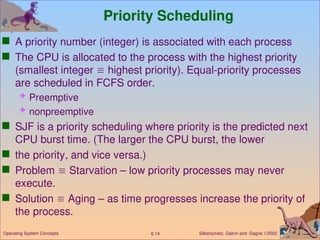
Priority Scheduling
 A priority number (integer) is associated with each process
 The CPU is allocated to the process with the highest priority
(smallest integer  highest priority). Equal-priority processes
are scheduled in FCFS order.
 Preemptive
 nonpreemptive
 SJF is a priority scheduling where priority is the predicted next
CPU burst time. (The larger the CPU burst, the lower
 the priority, and vice versa.)
 Problem  Starvation – low priority processes may never
execute.
 Solution  Aging – as time progresses increase the priority of
the process.

6.15
Round Robin (RR)
 Each process gets a small unit of CPU time (time quantum),
usually 10-100 milliseconds. After this time has elapsed, the
process is preempted and added to the end of the ready queue.
 If there are n processes in the ready queue and the time
quantum is q, then each process gets 1/n of the CPU time in
chunks of at most q time units at once. No process waits more
than (n-1)q time units.
 Performance
 q large  FIFO
 q small  q must be large with respect to context switch,
otherwise overhead is too high.

6.16
Example of RR with Time Quantum = 20
Process Burst Time
P1 53
P2 17
P3 68
P4 24
 The Gantt chart is:
 Typically, higher average turnaround than SJF, but better response.
P1 P2 P3 P4 P1 P3 P4 P1 P3 P3
0 20 37 57 77 97 117 121 134 154 162

6.17
Time Quantum and Context Switch Time

6.18
Turnaround Time Varies With The Time Quantum

6.19
Multilevel Queue
 Ready queue is partitioned into separate queues:
foreground (interactive)
background (batch)
 Each queue has its own scheduling algorithm,
foreground – RR
background – FCFS
 Scheduling must be done between the queues.
 Fixed priority scheduling; (i.e., serve all from foreground then from
background). Possibility of starvation.
 Time slice – each queue gets a certain amount of CPU time which
it can schedule amongst its processes; i.e., 80% to foreground in
RR 20% to background in FCFS

6.20
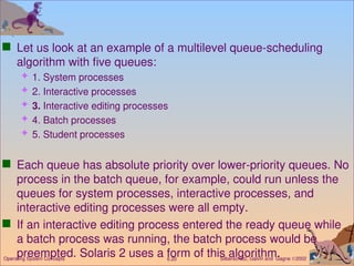
 Let us look at an example of a multilevel queue-scheduling
algorithm with five queues:
 1. System processes
 2. Interactive processes
 3. Interactive editing processes
 4. Batch processes
 5. Student processes
 Each queue has absolute priority over lower-priority queues. No
process in the batch queue, for example, could run unless the
queues for system processes, interactive processes, and
interactive editing processes were all empty.
 If an interactive editing process entered the ready queue while
a batch process was running, the batch process would be
preempted. Solaris 2 uses a form of this algorithm.

6.21
Multilevel Queue Scheduling

6.22
Multilevel Feedback Queue
 A process can move between the various queues; aging can be
implemented this way.
 Multilevel-feedback-queue scheduler defined by the following
parameters:
 number of queues
 scheduling algorithms for each queue
 method used to determine when to upgrade a process
 method used to determine when to demote a process
 method used to determine which queue a process will enter when
that process needs service

6.23
Example of Multilevel Feedback Queue
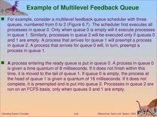
 For example, consider a multilevel feedback queue scheduler with three
queues, numbered from 0 to 2 (Figure 6.7). The scheduler first executes all
processes in queue 0. Only when queue 0 is empty will it execute processes
in queue 1. Similarly, processes in queue 2 will be executed only if queues 0
and 1 are empty. A process that arrives for queue 1 will preempt a process
in queue 2. A process that arrives for queue 0 will, in turn, preempt a
process in queue 1.
 A process entering the ready queue is put in queue 0. A process in queue 0
is given a time quantum of 8 milliseconds. If it does not finish within this
time, it is moved to the tail of queue 1. If queue 0 is empty, the process at
the head of queue 1 is given a quantum of 16 milliseconds. If it does not
complete, it is preempted and is put into queue 2. Processes in queue 2 are
run on an FCFS basis, only when queues 0 and 1 are empty.

6.24
Example of Multilevel Feedback Queue
 This scheduling algorithm gives highest priority to any process with a CPU
burst of 8 milliseconds or less. Such a process will quickly get the CPU,
finish its CPU burst, and go off to its next I/O burst. Processes that need
more than 8, but less than 16, milliseconds are also served quickly,
although with lower priority than shorter processes. Long processes
automatically sink to queue 2 and are served in FCFS order with any CPU
cycles left over from queues 0 and 1.

6.25
Figure 6.7

6.26
Multiple-Processor Scheduling
 CPU scheduling more complex when multiple CPUs are available.
 Homogeneous processors within a multiprocessor: We concentrate on
systems where the processors are identical (or homogeneous) in terms of
their functionality; any available processor can then be used to run any
processes in the queue.
 Load sharing : If several identical processors are available, then load
sharing can occur. It would be possible to provide a separate queue for
each processor. In this case, however, one processor could be idle, with an
empty queue, while another processor was very busy. To prevent this
situation, we use a common ready queue. All processes go into one queue
and are scheduled onto any available processor.
 Asymmetric multiprocessing – only one processor accesses the system data
structures, alleviating the need for data sharing. having all scheduling
decisions, I/O processing, and other system activities handled by one single
processor-the master server. The other processors only execute user code.

6.27
Real-Time Scheduling
 Hard real-time systems – required to complete a critical
task within a guaranteed amount of time.
 Soft real-time computing – requires that critical processes
receive priority over less fortunate(‫حظا‬ ‫)أقل‬ ones.

6.28
Dispatch Latency
 Dispatch latency – time it takes for the dispatcher to stop one process and
start another running.
 The conflict phase of dispatch latency has two components:
 1. Preemption of any process running in the kernel
 2. Release by low-priority processes resources needed by the high-priority process

6.29
Algorithm Evaluation
 How do we select a CPU-scheduling algorithm for a particular system? .
 The first problem is defining the criteria to be used in selecting an algorithm.
Criteria are often defined in terms of CPU utilization, response time, or
throughput.
 To select an algorithm, we must first define the relative importance of these
measures. Our criteria may include several measures, such as:
 Maximize CPU utilization under the constraint that the maximum response time is
1 second.
 Maximize throughput such that turnaround time is (on average) linearly
proportional to total execution time.
 Once the selection criteria have been defined, we want to evaluate the
various algorithms under consideration.

Operating System CPU Scheduling slide with OS

More Related Content

Similar to Operating System CPU Scheduling slide with OS

More from lovepreet33653

Recently uploaded

Operating System CPU Scheduling slide with OS