CPU Scheduling Algorithms of Operating Systems

Operating System Concepts Silberschatz and Galvin1999
5.1
Module 5: CPU Scheduling
• Basic Concepts
• Scheduling Criteria
• Scheduling Algorithms
• Multiple-Processor Scheduling
• Real-Time Scheduling
• Algorithm Evaluation

5.2
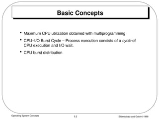
Basic Concepts
• Maximum CPU utilization obtained with multiprogramming
• CPU–I/O Burst Cycle – Process execution consists of a cycle of
CPU execution and I/O wait.
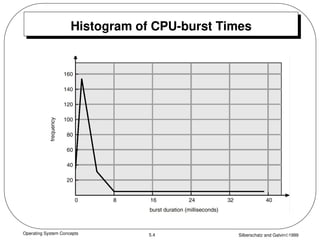
• CPU burst distribution

5.3
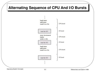
Alternating Sequence of CPU And I/O Bursts

5.4
Histogram of CPU-burst Times

5.5
CPU Scheduler
• Selects from among the processes in memory that are ready to
execute, and allocates the CPU to one of them.
• CPU scheduling decisions may take place when a process:
1. Switches from running to waiting state.
2. Switches from running to ready state.
3. Switches from waiting to ready.
4. Terminates.
• Scheduling under 1 and 4 is nonpreemptive.
• All other scheduling is preemptive.

5.6
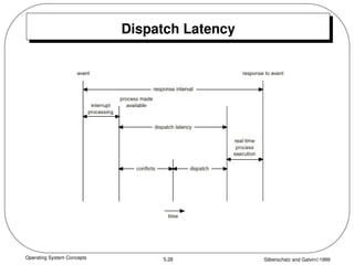
Dispatcher
• Dispatcher module gives control of the CPU to the process
selected by the short-term scheduler; this involves:
– switching context
– switching to user mode
– jumping to the proper location in the user program to restart
that program
• Dispatch latency – time it takes for the dispatcher to stop one
process and start another running.

5.7
Scheduling Criteria
• CPU utilization – keep the CPU as busy as possible
• Throughput – # of processes that complete their execution per
time unit
• Turnaround time – amount of time to execute a particular process
• Waiting time – amount of time a process has been waiting in the
ready queue
• Response time – amount of time it takes from when a request
was submitted until the first response is produced, not output
(for time-sharing environment)

5.8
Optimization Criteria
• Max CPU utilization
• Max throughput
• Min turnaround time
• Min waiting time
• Min response time

5.9
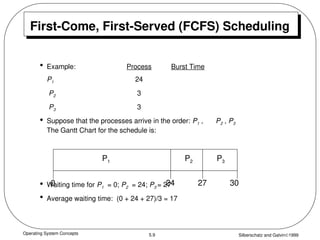
First-Come, First-Served (FCFS) Scheduling
• Example: Process Burst Time
P1 24
P2 3
P3 3
• Suppose that the processes arrive in the order: P1 , P2 , P3
The Gantt Chart for the schedule is:
• Waiting time for P1 = 0; P2 = 24; P3 = 27
• Average waiting time: (0 + 24 + 27)/3 = 17
P1 P2 P3
24 27 30
0

5.10
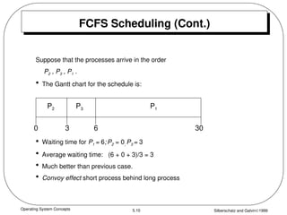
FCFS Scheduling (Cont.)
Suppose that the processes arrive in the order
P2 , P3 , P1 .
• The Gantt chart for the schedule is:
• Waiting time for P1 = 6; P2 = 0; P3 = 3
• Average waiting time: (6 + 0 + 3)/3 = 3
• Much better than previous case.
• Convoy effect short process behind long process
P1
P3
P2
6
3 30
0

5.11
Shortest-Job-First (SJR) Scheduling
• Associate with each process the length of its next CPU burst.
Use these lengths to schedule the process with the shortest time.
• Two schemes:
– nonpreemptive – once CPU given to the process it cannot
be preempted until completes its CPU burst.
– Preemptive – if a new process arrives with CPU burst length
less than remaining time of current executing process,
preempt. This scheme is know as the
Shortest-Remaining-Time-First (SRTF).
• SJF is optimal – gives minimum average waiting time for a given
set of processes.

5.12
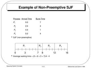
Process Arrival Time Burst Time
P1 0.0 7
P2 2.0 4
P3 4.0 1
P4 5.0 4
• SJF (non-preemptive)
• Average waiting time = (0 + 6 + 3 + 7)/4 - 4
Example of Non-Preemptive SJF
P1 P3 P2
7
3 16
0
P4
8 12

5.13
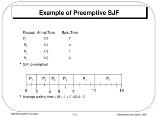
Example of Preemptive SJF
Process Arrival Time Burst Time
P1 0.0 7
P2 2.0 4
P3 4.0 1
P4 5.0 4
• SJF (preemptive)
• Average waiting time = (9 + 1 + 0 +2)/4 - 3
P1 P3
P2
4
2 11
0
P4
5 7
P2 P1
16

5.14
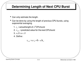
Determining Length of Next CPU Burst
• Can only estimate the length.
• Can be done by using the length of previous CPU bursts, using
exponential averaging.
:
Define
4.
1
0
,
3.
burst
CPU
next
the
for
value
predicted
2.
burst
CPU
of
lenght
actual
1.







 1
n
th
n n
t
  .
t n
n
n 


 


 1
1

5.15
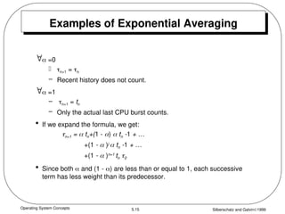
Examples of Exponential Averaging
 =0
 n+1 = n
– Recent history does not count.
 =1
– n+1 = tn
– Only the actual last CPU burst counts.
• If we expand the formula, we get:
n+1 =  tn+(1 - )  tn -1 + …
+(1 -  )j
 tn -1 + …
+(1 -  )n=1
tn 0
• Since both  and (1 - ) are less than or equal to 1, each successive
term has less weight than its predecessor.

5.16
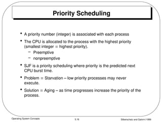
Priority Scheduling
• A priority number (integer) is associated with each process
• The CPU is allocated to the process with the highest priority
(smallest integer  highest priority).
– Preemptive
– nonpreemptive
• SJF is a priority scheduling where priority is the predicted next
CPU burst time.
• Problem  Starvation – low priority processes may never
execute.
• Solution  Aging – as time progresses increase the priority of the
process.

5.17
Round Robin (RR)
• Each process gets a small unit of CPU time (time quantum),
usually 10-100 milliseconds. After this time has elapsed, the
process is preempted and added to the end of the ready queue.
• If there are n processes in the ready queue and the time
quantum is q, then each process gets 1/n of the CPU time in
chunks of at most q time units at once. No process waits more
than (n-1)q time units.
• Performance
– q large  FIFO
– q small  q must be large with respect to context switch,
otherwise overhead is too high.

5.18
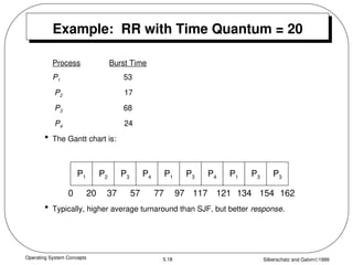
Example: RR with Time Quantum = 20
Process Burst Time
P1 53
P2 17
P3 68
P4 24
• The Gantt chart is:
• Typically, higher average turnaround than SJF, but better response.
P1 P2 P3 P4 P1 P3 P4 P1 P3 P3
0 20 37 57 77 97 117 121 134 154 162

5.19
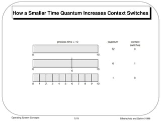
How a Smaller Time Quantum Increases Context Switches

5.20
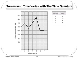
Turnaround Time Varies With The Time Quantum

5.21
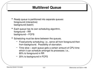
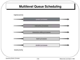
Multilevel Queue
• Ready queue is partitioned into separate queues:
foreground (interactive)
background (batch)
• Each queue has its own scheduling algorithm,
foreground – RR
background – FCFS
• Scheduling must be done between the queues.
– Fixed priority scheduling; i.e., serve all from foreground then
from background. Possibility of starvation.
– Time slice – each queue gets a certain amount of CPU time
which it can schedule amongst its processes; i.e.,
80% to foreground in RR
– 20% to background in FCFS

5.22
Multilevel Queue Scheduling

5.23
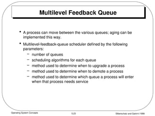
Multilevel Feedback Queue
• A process can move between the various queues; aging can be
implemented this way.
• Multilevel-feedback-queue scheduler defined by the following
parameters:
– number of queues
– scheduling algorithms for each queue
– method used to determine when to upgrade a process
– method used to determine when to demote a process
– method used to determine which queue a process will enter
when that process needs service

5.24
Multilevel Feedback Queues

5.25
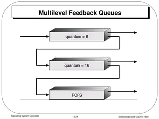
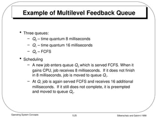
Example of Multilevel Feedback Queue
• Three queues:
– Q0 – time quantum 8 milliseconds
– Q1 – time quantum 16 milliseconds
– Q2 – FCFS
• Scheduling
– A new job enters queue Q0 which is served FCFS. When it
gains CPU, job receives 8 milliseconds. If it does not finish
in 8 milliseconds, job is moved to queue Q1.
– At Q1 job is again served FCFS and receives 16 additional
milliseconds. If it still does not complete, it is preempted
and moved to queue Q2.

5.26
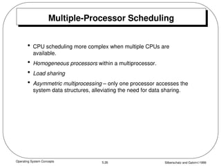
Multiple-Processor Scheduling
• CPU scheduling more complex when multiple CPUs are
available.
• Homogeneous processors within a multiprocessor.
• Load sharing
• Asymmetric multiprocessing – only one processor accesses the
system data structures, alleviating the need for data sharing.

5.27
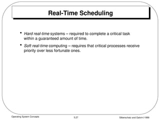
Real-Time Scheduling
• Hard real-time systems – required to complete a critical task
within a guaranteed amount of time.
• Soft real-time computing – requires that critical processes receive
priority over less fortunate ones.

5.28
Dispatch Latency

5.29
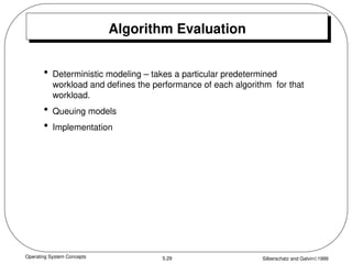
Algorithm Evaluation
• Deterministic modeling – takes a particular predetermined
workload and defines the performance of each algorithm for that
workload.
• Queuing models
• Implementation

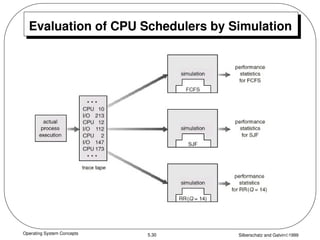
5.30
Evaluation of CPU Schedulers by Simulation

CPU Scheduling Algorithms of Operating Systems

More Related Content

Similar to CPU Scheduling Algorithms of Operating Systems

Recently uploaded

CPU Scheduling Algorithms of Operating Systems