ch6.ppt

Silberschatz, Galvin and Gagne ©2013
Operating System Concepts – 9th Edition
Chapter 6: CPU Scheduling

6.2 Silberschatz, Galvin and Gagne ©2013
Chapter 6: CPU Scheduling
 Basic Concepts
 Scheduling Criteria
 Scheduling Algorithms
 Thread Scheduling
 Multiple-Processor Scheduling
 Real-Time CPU Scheduling
 Operating Systems Examples
 Algorithm Evaluation

Objectives
 To introduce CPU scheduling, which is the basis for
multiprogrammed operating systems
 To describe various CPU-scheduling algorithms
 To discuss evaluation criteria for selecting a CPU-scheduling
algorithm for a particular system
 To examine the scheduling algorithms of several operating
systems

Basic Concepts
 Maximum CPU utilization
obtained with multiprogramming
 CPU–I/O Burst Cycle – Process
execution consists of a cycle of
CPU execution and I/O wait
 CPU burst followed by I/O burst
 CPU burst distribution is of main
concern

Histogram of CPU-burst Times

CPU Scheduler
 Short-term scheduler selects from among the processes in
ready queue, and allocates the CPU to one of them
 Queue may be ordered in various ways
 CPU scheduling decisions may take place when a process:
1. Switches from running to waiting state
2. Switches from running to ready state
3. Switches from waiting to ready
4. Terminates
 Scheduling under 1 and 4 is nonpreemptive
 All other scheduling is preemptive
 Consider access to shared data
 Consider preemption while in kernel mode
 Consider interrupts occurring during crucial OS activities

Dispatcher
 Dispatcher module gives control of the CPU to the process
selected by the short-term scheduler; this involves:
 switching context
 switching to user mode
 jumping to the proper location in the user program to
restart that program
 Dispatch latency – time it takes for the dispatcher to stop
one process and start another running

Scheduling Criteria
 CPU utilization – keep the CPU as busy as possible
 Throughput – # of processes that complete their execution per
time unit
 Turnaround time – amount of time to execute a particular
process
 Waiting time – amount of time a process has been waiting in the
ready queue
 Response time – amount of time it takes from when a request
was submitted until the first response is produced, not output (for
time-sharing environment)

Scheduling Algorithm Optimization Criteria
 Max CPU utilization
 Max throughput
 Min turnaround time
 Min waiting time
 Min response time

First- Come, First-Served (FCFS) Scheduling
Process Burst Time
P1 24
P2 3
P3 3
 Suppose that the processes arrive in the order: P1 , P2 , P3
The Gantt Chart for the schedule is:
 Waiting time for P1 = 0; P2 = 24; P3 = 27
 Average waiting time: (0 + 24 + 27)/3 = 17
P P P
1 2 3
0 24 30
27

FCFS Scheduling (Cont.)
Suppose that the processes arrive in the order:
P2 , P3 , P1
 The Gantt chart for the schedule is:
 Waiting time for P1 = 6; P2 = 0; P3 = 3
 Average waiting time: (6 + 0 + 3)/3 = 3
 Much better than previous case
 Convoy effect - short process behind long process
 Consider one CPU-bound and many I/O-bound processes
P1
0 3 6 30
P2
P3

Shortest-Job-First (SJF) Scheduling
 Associate with each process the length of its next CPU burst
 Use these lengths to schedule the process with the shortest
time
 SJF is optimal – gives minimum average waiting time for a given
set of processes
 The difficulty is knowing the length of the next CPU request
 Could ask the user

Example of SJF
ProcessArrival Time Burst Time
P1 0.0 6
P2 2.0 8
P3 4.0 7
P4 5.0 3
 SJF scheduling chart
 Average waiting time = (3 + 16 + 9 + 0) / 4 = 7
P3
0 3 24
P4
P1
16
9
P2

Determining Length of Next CPU Burst
 Can only estimate the length – should be similar to the previous one
 Then pick process with shortest predicted next CPU burst
 Can be done by using the length of previous CPU bursts, using
exponential averaging
 Commonly, α set to ½
 Preemptive version called shortest-remaining-time-first
:
Define
4.
1
0
,
3.
burst
CPU
next
the
for
value
predicted
2.
burst
CPU
of
length
actual
1.







 1
n
th
n n
t
  .
1
1 n
n
n
t 


 




Prediction of the Length of the Next CPU Burst

Examples of Exponential Averaging
  =0
 n+1 = n
 Recent history does not count
  =1
 n+1 =  tn
 Only the actual last CPU burst counts
 If we expand the formula, we get:
n+1 =  tn+(1 - ) tn -1 + …
+(1 -  )j  tn -j + …
+(1 -  )n +1 0
 Since both  and (1 - ) are less than or equal to 1, each
successive term has less weight than its predecessor

Example of Shortest-remaining-time-first
 Now we add the concepts of varying arrival times and preemption to
the analysis
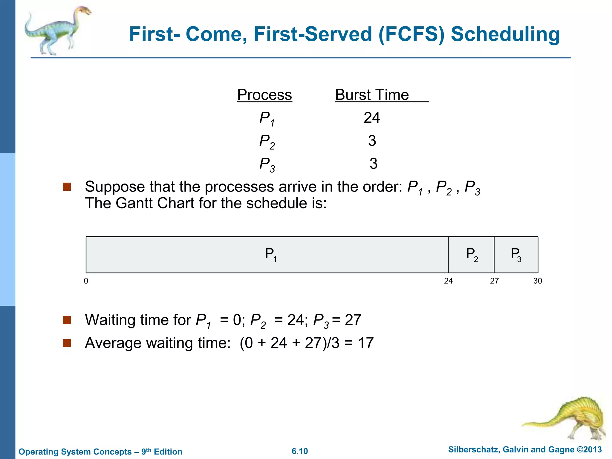
ProcessAarri Arrival TimeT Burst Time
P1 0 8
P2 1 4
P3 2 9
P4 3 5
 Preemptive SJF Gantt Chart
 Average waiting time = [(10-1)+(1-1)+(17-2)+5-3)]/4 = 26/4 = 6.5
msec
P4
0 1 26
P1
P2
10
P3
P1
5 17

Priority Scheduling
 A priority number (integer) is associated with each process
 The CPU is allocated to the process with the highest priority
(smallest integer  highest priority)
 Preemptive
 Nonpreemptive
 SJF is priority scheduling where priority is the inverse of predicted
next CPU burst time
 Problem  Starvation – low priority processes may never execute
 Solution  Aging – as time progresses increase the priority of the
process

Example of Priority Scheduling
ProcessA arri Burst TimeT Priority
P1 10 3
P2 1 1
P3 2 4
P4 1 5
P5 5 2
 Priority scheduling Gantt Chart
 Average waiting time = 8.2 msec

Round Robin (RR)
 Each process gets a small unit of CPU time (time quantum q),
usually 10-100 milliseconds. After this time has elapsed, the
process is preempted and added to the end of the ready queue.
 If there are n processes in the ready queue and the time
quantum is q, then each process gets 1/n of the CPU time in
chunks of at most q time units at once. No process waits more
than (n-1)q time units.
 Timer interrupts every quantum to schedule next process
 Performance
 q large  FIFO
 q small  q must be large with respect to context switch,
otherwise overhead is too high

Example of RR with Time Quantum = 4
Process Burst Time
P1 24
P2 3
P3 3
 The Gantt chart is:
 Typically, higher average turnaround than SJF, but better
response
 q should be large compared to context switch time
 q usually 10ms to 100ms, context switch < 10 usec
P P P
1 1 1
0 18 30
26
14
4 7 10 22
P2
P3
P1
P1
P1

Time Quantum and Context Switch Time

Turnaround Time Varies With The Time Quantum
80% of CPU bursts
should be shorter than q

Multilevel Queue
 Ready queue is partitioned into separate queues, eg:
 foreground (interactive)
 background (batch)
 Process permanently in a given queue
 Each queue has its own scheduling algorithm:
 foreground – RR
 background – FCFS
 Scheduling must be done between the queues:
 Fixed priority scheduling; (i.e., serve all from foreground then
from background). Possibility of starvation.
 Time slice – each queue gets a certain amount of CPU time
which it can schedule amongst its processes; i.e., 80% to
foreground in RR
 20% to background in FCFS

Multilevel Queue Scheduling

Multilevel Feedback Queue
 A process can move between the various queues; aging can be
implemented this way
 Multilevel-feedback-queue scheduler defined by the following
parameters:
 number of queues
 scheduling algorithms for each queue
 method used to determine when to upgrade a process
 method used to determine when to demote a process
 method used to determine which queue a process will enter
when that process needs service

Example of Multilevel Feedback Queue
 Three queues:
 Q0 – RR with time quantum 8
milliseconds
 Q1 – RR time quantum 16 milliseconds
 Q2 – FCFS
 Scheduling
 A new job enters queue Q0 which is
served FCFS
 When it gains CPU, job receives 8
milliseconds
 If it does not finish in 8
milliseconds, job is moved to
queue Q1
 At Q1 job is again served FCFS and
receives 16 additional milliseconds
 If it still does not complete, it is
preempted and moved to queue Q2

Thread Scheduling
 Distinction between user-level and kernel-level threads
 When threads supported, threads scheduled, not processes
 Many-to-one and many-to-many models, thread library schedules
user-level threads to run on LWP
 Known as process-contention scope (PCS) since scheduling
competition is within the process
 Typically done via priority set by programmer
 Kernel thread scheduled onto available CPU is system-contention
scope (SCS) – competition among all threads in system

Pthread Scheduling
 API allows specifying either PCS or SCS during thread creation
 PTHREAD_SCOPE_PROCESS schedules threads using
PCS scheduling
 PTHREAD_SCOPE_SYSTEM schedules threads using
SCS scheduling
 Can be limited by OS – Linux and Mac OS X only allow
PTHREAD_SCOPE_SYSTEM

Pthread Scheduling API
#include <pthread.h>
#include <stdio.h>
#define NUM_THREADS 5
int main(int argc, char *argv[]) {
int i, scope;
pthread_t tid[NUM THREADS];
pthread_attr_t attr;
/* get the default attributes */
pthread_attr_init(&attr);
/* first inquire on the current scope */
if (pthread_attr_getscope(&attr, &scope) != 0)
fprintf(stderr, "Unable to get scheduling scopen");
else {
if (scope == PTHREAD_SCOPE_PROCESS)
printf("PTHREAD_SCOPE_PROCESS");
else if (scope == PTHREAD_SCOPE_SYSTEM)
printf("PTHREAD_SCOPE_SYSTEM");
else
fprintf(stderr, "Illegal scope value.n");
}

Pthread Scheduling API
/* set the scheduling algorithm to PCS or SCS */
pthread_attr_setscope(&attr, PTHREAD_SCOPE_SYSTEM);
/* create the threads */
for (i = 0; i < NUM_THREADS; i++)
pthread_create(&tid[i],&attr,runner,NULL);
/* now join on each thread */
pthread_join(tid[i], NULL);
}
/* Each thread will begin control in this function */
void *runner(void *param)
{
/* do some work ... */
pthread_exit(0);
}

Multiple-Processor Scheduling
 CPU scheduling more complex when multiple CPUs are
available
 Homogeneous processors within a multiprocessor
 Asymmetric multiprocessing – only one processor accesses
the system data structures, alleviating the need for data sharing
 Symmetric multiprocessing (SMP) – each processor is self-
scheduling, all processes in common ready queue, or each has
its own private queue of ready processes
 Currently, most common
 Processor affinity – process has affinity for processor on which
it is currently running
 soft affinity
 hard affinity
 Variations including processor sets

NUMA and CPU Scheduling
Note that memory-placement algorithms can also consider affinity

Multiple-Processor Scheduling – Load Balancing
 If SMP, need to keep all CPUs loaded for efficiency
 Load balancing attempts to keep workload evenly distributed
 Push migration – periodic task checks load on each processor,
and if found pushes task from overloaded CPU to other CPUs
 Pull migration – idle processors pulls waiting task from busy
processor

Multicore Processors
 Recent trend to place multiple processor cores on same
physical chip
 Faster and consumes less power
 Multiple threads per core also growing
 Takes advantage of memory stall to make progress on
another thread while memory retrieve happens

Multithreaded Multicore System

Real-Time CPU Scheduling
 Can present obvious
challenges
 Soft real-time systems – no
guarantee as to when critical
real-time process will be
scheduled
 Hard real-time systems –
task must be serviced by its
deadline
 Two types of latencies affect
performance
1. Interrupt latency – time from
arrival of interrupt to start of
routine that services interrupt
2. Dispatch latency – time for
schedule to take current process
off CPU and switch to another

Real-Time CPU Scheduling (Cont.)
 Conflict phase of
dispatch latency:
1. Preemption of
any process
running in kernel
mode
2. Release by low-
priority process
of resources
needed by high-
priority
processes

Priority-based Scheduling
 For real-time scheduling, scheduler must support preemptive, priority-
based scheduling
 But only guarantees soft real-time
 For hard real-time must also provide ability to meet deadlines
 Processes have new characteristics: periodic ones require CPU at
constant intervals
 Has processing time t, deadline d, period p
 0 ≤ t ≤ d ≤ p
 Rate of periodic task is 1/p

Virtualization and Scheduling
 Virtualization software schedules multiple guests onto
CPU(s)
 Each guest doing its own scheduling
 Not knowing it doesn’t own the CPUs
 Can result in poor response time
 Can effect time-of-day clocks in guests
 Can undo good scheduling algorithm efforts of guests

Rate Montonic Scheduling
 A priority is assigned based on the inverse of its period
 Shorter periods = higher priority;
 Longer periods = lower priority
 P1 is assigned a higher priority than P2.

Missed Deadlines with Rate Monotonic Scheduling

Earliest Deadline First Scheduling (EDF)
 Priorities are assigned according to deadlines:
the earlier the deadline, the higher the priority;
the later the deadline, the lower the priority

Proportional Share Scheduling
 T shares are allocated among all processes in the system
 An application receives N shares where N < T
 This ensures each application will receive N / T of the total
processor time

POSIX Real-Time Scheduling
 The POSIX.1b standard
 API provides functions for managing real-time threads
 Defines two scheduling classes for real-time threads:
1. SCHED_FIFO - threads are scheduled using a FCFS strategy with a
FIFO queue. There is no time-slicing for threads of equal priority
2. SCHED_RR - similar to SCHED_FIFO except time-slicing occurs for
threads of equal priority
 Defines two functions for getting and setting scheduling policy:
1. pthread_attr_getsched_policy(pthread_attr_t *attr,
int *policy)
2. pthread_attr_setsched_policy(pthread_attr_t *attr,
int policy)

POSIX Real-Time Scheduling API
#include <pthread.h>
#include <stdio.h>
#define NUM_THREADS 5
int main(int argc, char *argv[])
{
int i, policy;
pthread_t_tid[NUM_THREADS];
pthread_attr_t attr;
/* get the default attributes */
pthread_attr_init(&attr);
/* get the current scheduling policy */
if (pthread_attr_getschedpolicy(&attr, &policy) != 0)
fprintf(stderr, "Unable to get policy.n");
else {
if (policy == SCHED_OTHER) printf("SCHED_OTHERn");
else if (policy == SCHED_RR) printf("SCHED_RRn");
else if (policy == SCHED_FIFO) printf("SCHED_FIFOn");
}

POSIX Real-Time Scheduling API (Cont.)
/* set the scheduling policy - FIFO, RR, or OTHER */
if (pthread_attr_setschedpolicy(&attr, SCHED_FIFO) != 0)
fprintf(stderr, "Unable to set policy.n");
/* create the threads */
pthread_create(&tid[i],&attr,runner,NULL);
/* now join on each thread */
pthread_join(tid[i], NULL);
}
/* Each thread will begin control in this function */
void *runner(void *param)
{
/* do some work ... */
pthread_exit(0);
}

Operating System Examples
 Linux scheduling
 Windows scheduling
 Solaris scheduling

Linux Scheduling Through Version 2.5
 Prior to kernel version 2.5, ran variation of standard UNIX
scheduling algorithm
 Version 2.5 moved to constant order O(1) scheduling time
 Preemptive, priority based
 Two priority ranges: time-sharing and real-time
 Real-time range from 0 to 99 and nice value from 100 to 140
 Map into global priority with numerically lower values indicating higher
priority
 Higher priority gets larger q
 Task run-able as long as time left in time slice (active)
 If no time left (expired), not run-able until all other tasks use their slices
 All run-able tasks tracked in per-CPU runqueue data structure
 Two priority arrays (active, expired)
 Tasks indexed by priority
 When no more active, arrays are exchanged
 Worked well, but poor response times for interactive processes

Linux Scheduling in Version 2.6.23 +
 Completely Fair Scheduler (CFS)
 Scheduling classes
 Each has specific priority
 Scheduler picks highest priority task in highest scheduling class
 Rather than quantum based on fixed time allotments, based on proportion of CPU
time
 2 scheduling classes included, others can be added
1. default
2. real-time
 Quantum calculated based on nice value from -20 to +19
 Lower value is higher priority
 Calculates target latency – interval of time during which task should run at least
once
 Target latency can increase if say number of active tasks increases
 CFS scheduler maintains per task virtual run time in variable vruntime
 Associated with decay factor based on priority of task – lower priority is higher
decay rate
 Normal default priority yields virtual run time = actual run time
 To decide next task to run, scheduler picks task with lowest virtual run time

CFS Performance

Linux Scheduling (Cont.)
 Real-time scheduling according to POSIX.1b
 Real-time tasks have static priorities
 Real-time plus normal map into global priority scheme
 Nice value of -20 maps to global priority 100
 Nice value of +19 maps to priority 139

Windows Scheduling
 Windows uses priority-based preemptive scheduling
 Highest-priority thread runs next
 Dispatcher is scheduler
 Thread runs until (1) blocks, (2) uses time slice, (3)
preempted by higher-priority thread
 Real-time threads can preempt non-real-time
 32-level priority scheme
 Variable class is 1-15, real-time class is 16-31
 Priority 0 is memory-management thread
 Queue for each priority
 If no run-able thread, runs idle thread

Windows Priority Classes
 Win32 API identifies several priority classes to which a process can belong
 REALTIME_PRIORITY_CLASS, HIGH_PRIORITY_CLASS,
ABOVE_NORMAL_PRIORITY_CLASS,NORMAL_PRIORITY_CLASS,
BELOW_NORMAL_PRIORITY_CLASS, IDLE_PRIORITY_CLASS
 All are variable except REALTIME
 A thread within a given priority class has a relative priority
 TIME_CRITICAL, HIGHEST, ABOVE_NORMAL, NORMAL, BELOW_NORMAL,
LOWEST, IDLE
 Priority class and relative priority combine to give numeric priority
 Base priority is NORMAL within the class
 If quantum expires, priority lowered, but never below base

Windows Priority Classes (Cont.)
 If wait occurs, priority boosted depending on what was waited for
 Foreground window given 3x priority boost
 Windows 7 added user-mode scheduling (UMS)
 Applications create and manage threads independent of kernel
 For large number of threads, much more efficient
 UMS schedulers come from programming language libraries like
C++ Concurrent Runtime (ConcRT) framework

Windows Priorities

Solaris
 Priority-based scheduling
 Six classes available
 Time sharing (default) (TS)
 Interactive (IA)
 Real time (RT)
 System (SYS)
 Fair Share (FSS)
 Fixed priority (FP)
 Given thread can be in one class at a time
 Each class has its own scheduling algorithm
 Time sharing is multi-level feedback queue
 Loadable table configurable by sysadmin

Solaris Dispatch Table

Solaris Scheduling

Solaris Scheduling (Cont.)
 Scheduler converts class-specific priorities into a per-thread global
priority
 Thread with highest priority runs next
 Runs until (1) blocks, (2) uses time slice, (3) preempted by
higher-priority thread
 Multiple threads at same priority selected via RR

Algorithm Evaluation
 How to select CPU-scheduling algorithm for an OS?
 Determine criteria, then evaluate algorithms
 Deterministic modeling
 Type of analytic evaluation
 Takes a particular predetermined workload and defines the
performance of each algorithm for that workload
 Consider 5 processes arriving at time 0:

Deterministic Evaluation
 For each algorithm, calculate minimum average waiting time
 Simple and fast, but requires exact numbers for input, applies only to
those inputs
 FCS is 28ms:
 Non-preemptive SFJ is 13ms:
 RR is 23ms:

Queueing Models
 Describes the arrival of processes, and CPU and I/O bursts
probabilistically
 Commonly exponential, and described by mean
 Computes average throughput, utilization, waiting time, etc
 Computer system described as network of servers, each with
queue of waiting processes
 Knowing arrival rates and service rates
 Computes utilization, average queue length, average wait
time, etc

Little’s Formula
 n = average queue length
 W = average waiting time in queue
 λ = average arrival rate into queue
 Little’s law – in steady state, processes leaving queue must equal
processes arriving, thus:
n = λ x W
 Valid for any scheduling algorithm and arrival distribution
 For example, if on average 7 processes arrive per second, and
normally 14 processes in queue, then average wait time per
process = 2 seconds

Simulations
 Queueing models limited
 Simulations more accurate
 Programmed model of computer system
 Clock is a variable
 Gather statistics indicating algorithm performance
 Data to drive simulation gathered via
 Random number generator according to probabilities
 Distributions defined mathematically or empirically
 Trace tapes record sequences of real events in real systems

Evaluation of CPU Schedulers by Simulation

Implementation
 Even simulations have limited accuracy
 Just implement new scheduler and test in real systems
 High cost, high risk
 Environments vary
 Most flexible schedulers can be modified per-site or per-system
 Or APIs to modify priorities
 But again environments vary

ch6.ppt

More Related Content

Similar to ch6.ppt

More from Sami Mughal

Recently uploaded

ch6.ppt