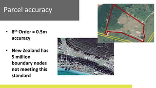
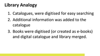
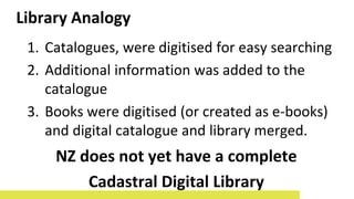
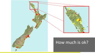
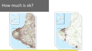
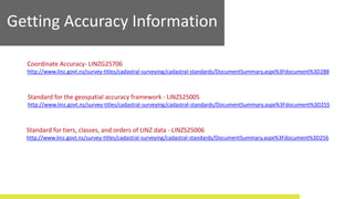
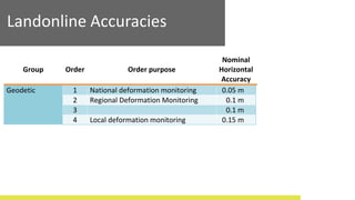
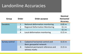
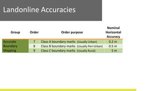
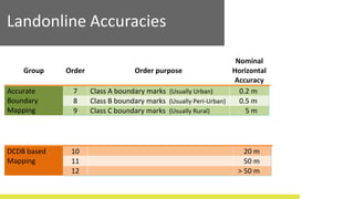
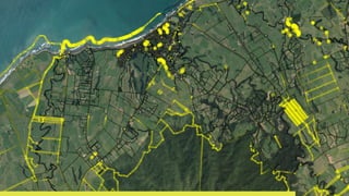
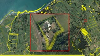
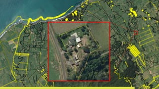
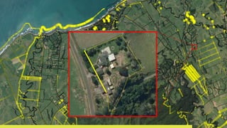
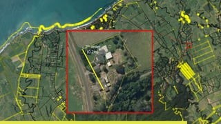
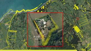
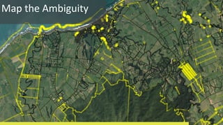
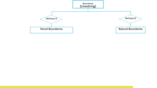
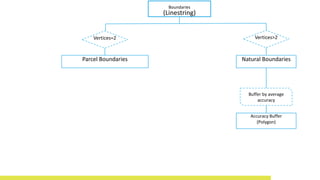
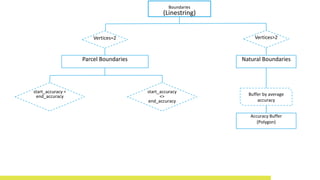
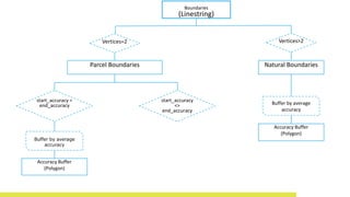
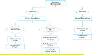
Parcel Boundaries:
Visualising the accuracy myth
Andrew Clouston| Geospatial Team Leader
Sisi Zhang | Geospatial Analyst
ESRI User Conference 2014, Auckland, 19 August 2014
Overview
- The Cadastre
- How much is accurate
- Obtaining accuracy information
- Node accuracy
- Visualising Accuracy
What is the New
Zealand Cadastre?
Other Crown
records to support
and define
boundaries
+
Parcel accuracy
Parcel accuracy
• 8th Order = 0.5m
accuracy
• New Zealand has
5 million
boundary nodes
not meeting this
standard
Background -
Indexes and Maps
Background -
Indexes and Maps
Library Analogy
1. Catalogues, were digitised for easy searching
Library Analogy
1. Catalogues, were digitised for easy searching
2. Additional information was added to the
catalogue
Library Analogy
1. Catalogues, were digitised for easy searching
2. Additional information was added to the
catalogue
3. Books were digitised (or created as e-books)
and digital catalogue and library merged.
Library Analogy
NZ does not yet have a complete
Cadastral Digital Library
1. Catalogues, were digitised for easy searching
2. Additional information was added to the
catalogue
3. Books were digitised (or created as e-books)
and digital catalogue and library merged.
Library Analogy
How much is ok?
How much is ok?
How much is ok?
How much is ok?
Getting Accuracy Information
Coordinate Accuracy- LINZG25706
http://www.linz.govt.nz/survey-titles/cadastral-surveying/cadastral-standards/DocumentSummary.aspx%3Fdocument%3D288
Standard for the geospatial accuracy framework - LINZS25005
http://www.linz.govt.nz/survey-titles/cadastral-surveying/cadastral-standards/DocumentSummary.aspx%3Fdocument%3D255
Standard for tiers, classes, and orders of LINZ data - LINZS25006
http://www.linz.govt.nz/survey-titles/cadastral-surveying/cadastral-standards/DocumentSummary.aspx%3Fdocument%3D256
Getting Accuracy Information
Landonline Accuracies
Group Order Order purpose
Nominal
Horizontal
Accuracy
Geodetic 1 National deformation monitoring 0.05 m
2 Regional Deformation Monitoring 0.1 m
3 0.1 m
4 Local deformation monitoring 0.15 m
Landonline Accuracies
Group Order Order purpose
Nominal
Horizontal
Accuracy
Geodetic 1 National deformation monitoring 0.05 m
2 Regional Deformation Monitoring 0.1 m
3 0.1 m
4 Local deformation monitoring 0.15 m
Survey control 5 Cadastral horizontal control and
Basic geospatial network
0.15 m
6 Cadastral permanent reference and
witness marks
0.15 m
Landonline Accuracies
Group Order Order purpose
Nominal
Horizontal
Accuracy
Accurate
Boundary
Mapping
7 Class A boundary marks (Usually Urban) 0.2 m
8 Class B boundary marks (Usually Peri-Urban) 0.5 m
9 Class C boundary marks (Usually Rural) 5 m
Landonline Accuracies
Group Order Order purpose
Nominal
Horizontal
Accuracy
Accurate
Boundary
Mapping
7 Class A boundary marks (Usually Urban) 0.2 m
8 Class B boundary marks (Usually Peri-Urban) 0.5 m
9 Class C boundary marks (Usually Rural) 5 m
DCDB based
Mapping
10 20 m
11 50 m
12 > 50 m
Thematic Node View
Thematic Node View
Nodes OK / Not Ok
Distortion
Map the Ambiguity
7th order
(0.2m)
7th order
(0.2m)
9th order
(5m)
7th order
(0.2m)
9th order
(5m)
7th order
(0.2m)
9th order
(5m)
7th order
(0.2m)
9th order
(5m)
Map the Ambiguity
The process
Boundaries
(Linestring)
Natural BoundariesParcel Boundaries
Vertices=2 Vertices>2
Boundaries
(Linestring)
Natural BoundariesParcel Boundaries
Vertices=2 Vertices>2
Buffer by average
accuracy
Accuracy Buffer
(Polygon)
Boundaries
(Linestring)
Natural BoundariesParcel Boundaries
Vertices=2 Vertices>2
Buffer by average
accuracy
Accuracy Buffer
(Polygon)
start_accuracy
<>
end_accuracy
start_accuracy =
end_accuracy
Boundaries
(Linestring)
Natural BoundariesParcel Boundaries
Vertices=2 Vertices>2
Buffer by average
accuracy
Accuracy Buffer
(Polygon)
Accuracy Buffer
(Polygon)
Buffer by average
accuracy
start_accuracy
<>
end_accuracy
start_accuracy =
end_accuracy
Boundaries
(Linestring)
Natural BoundariesParcel Boundaries
Vertices=2 Vertices>2
Buffer by average
accuracy
Accuracy Buffer
(Polygon)
Accuracy Buffer
(Polygon)
Buffer by average
accuracy
start_accuracy
<>
end_accuracy
start_accuracy =
end_accuracy
Accuracy Buffer
(Tropism Polygon)
Flag ‘Wrong Direction’
boundaries
Buffer by start and end
accuracy
Take home points
- Cadastral mapping is variable,
especially in rural areas
- Inaccuracy is not necessarily an error
- Accuracy information is on the LDS
- Accuracy can be visualised
Questions?

NZ parcel accuracy, visualising the accuracy myth

Editor's Notes

  • #4 The cadastre is much more than Cadastral Boundaries. These pictures give a sense of the scope and that it is much wider than just the LINZ records that people access
  • #5 The cadastre is much more than Cadastral Boundaries. These pictures give a sense of the scope and that it is much wider than just the LINZ records that people access
  • #15 Red is Survey capture areas at the time Landonline rolled out, yellow Spatial Parcel Improvement projects circs 2011. this is essentially 6% of NZ but is more than 70% of parcels and approx 50% of boundary marks.
  • #16 Red is Survey capture areas at the time Landonline rolled out, yellow Spatial Parcel Improvement projects circs 2011. this is essentially 6% of NZ but is more than 70% of parcels and approx 50% of boundary marks.
  • #17 Left: what it should be like Right : What it actually is (this map is parcel vectors - https://data.linz.govt.nz/layer/820-nz-survey-boundary-vectors/ )
  • #18 Left: what it should be like Right : What it actually is (this map is parcel vectors - https://data.linz.govt.nz/layer/820-nz-survey-boundary-vectors/ )
  • #19 The extends of cadastral adjustments is another useful layer, There are several, each with their own purposes- refer to the metadata. Search with the word ‘Adjustment’ will locate them
  • #20 The extends of cadastral adjustments is another useful layer, There are several, each with their own purposes- refer to the metadata. Search with the word ‘Adjustment’ will locate them
  • #22 Quick reference links for those that are interested. There is real benefits if everyone assigned the same accuracy values to their spatial data (along with a date of acquisition) so that data can be easily compared and contrasted.
  • #23 These orders are generally not boundary marks, and comprise approximately 0.5% of all nodes in the cadastre
  • #24 These orders are generally not boundary marks, and comprise approximately 0.5% of all nodes in the cadastre
  • #25 These orders are generally not boundary marks, and comprise approximately 0.5% of all nodes in the cadastre
  • #26 The accurate boundary mapping comprises of data capture when Landonline was build and subsequent surveys. The vast majority or order 7 and 8 (approximately 50%) of all nodes lie in survey capture areas. Note that the relative accuracies between these nodes is very good (usually sub decimeter) Order 10-12 nodes can generally trace their lineage back to DCDB mapping, however some new surveys that have been approved and not yet integrated will also be order 10, yet their accuracies will be ‘quite good’
  • #27 The accurate boundary mapping comprises of data capture when Landonline was build and subsequent surveys. The vast majority or order 7 and 8 (approximately 50%) of all nodes lie in survey capture areas. Note that the relative accuracies between these nodes is very good (usually sub decimeter) Order 10-12 nodes can generally trace their lineage back to DCDB mapping, however some new surveys that have been approved and not yet integrated will also be order 10, yet their accuracies will be ‘quite good’
  • #28 A thematic example of these nodes. Could be considered a bare minimum for user information. This is a poor visualisation as it is relatively unhelpful for most users (too much colour) but is better than nothing
  • #29 A thematic example of these nodes. Could be considered a bare minimum for user information. This is a poor visualisation as it is relatively unhelpful for most users (too much colour) but is better than nothing
  • #30 A thematic example of these nodes. This is a better representation where the thematic that groups orders 7-9 together for ‘trusted nodes’ and ‘10-12’ for untrusted nodes. Sometime less is more!!
  • #31 Comparing the survey areas to the geometric area can identify differences. This map shows the diference (plus or minus) 1-10%. Larger differences usually relate to parcels where the survey area listed may not be correct. This is a crude analysis that highlights distortion
  • #32 Comparing the survey areas to the geometric area can identify differences. This map shows the diference (plus or minus) 1-10%. Larger differences usually relate to parcels where the survey area listed may not be correct. This is a crude analysis that highlights distortion
  • #33 A better may to visualise the data. Note, The mapping in this example is actually slight worse than the orders would indicate. But it clearly indicates to users the southern boundaries are poorly mapped and should not be relied on
  • #34 A better may to visualise the data. Note, The mapping in this example is actually slight worse than the orders would indicate. But it clearly indicates to users the southern boundaries are poorly mapped and should not be relied on
  • #35 A better may to visualise the data. Note, The mapping in this example is actually slight worse than the orders would indicate. But it clearly indicates to users the southern boundaries are poorly mapped and should not be relied on
  • #36 A better may to visualise the data. Note, The mapping in this example is actually slight worse than the orders would indicate. But it clearly indicates to users the southern boundaries are poorly mapped and should not be relied on
  • #37 A better may to visualise the data. Note, The mapping in this example is actually slight worse than the orders would indicate. But it clearly indicates to users the southern boundaries are poorly mapped and should not be relied on
  • #38 A better may to visualise the data. Note, The mapping in this example is actually slight worse than the orders would indicate. But it clearly indicates to users the southern boundaries are poorly mapped and should not be relied on
  • #39 A better may to visualise the data. Note, The mapping in this example is actually slight worse than the orders would indicate. But it clearly indicates to users the southern boundaries are poorly mapped and should not be relied on
  • #40 A better may to visualise the data. Note, The mapping in this example is actually slight worse than the orders would indicate. But it clearly indicates to users the southern boundaries are poorly mapped and should not be relied on
  • #41 A better may to visualise the data. Note, The mapping in this example is actually slight worse than the orders would indicate. But it clearly indicates to users the southern boundaries are poorly mapped and should not be relied on
  • #42 A better may to visualise the data. Note, The mapping in this example is actually slight worse than the orders would indicate. But it clearly indicates to users the southern boundaries are poorly mapped and should not be relied on
  • #43 A better may to visualise the data. Note, The mapping in this example is actually slight worse than the orders would indicate. But it clearly indicates to users the southern boundaries are poorly mapped and should not be relied on
  • #45 Diagrammatic methodology for creating the buffers. Note this requires the use of large datasets and the ability to use the full Landonline marks and observations datasets.
  • #46 Diagrammatic methodology for creating the buffers. Note this requires the use of large datasets and the ability to use the full Landonline marks and observations datasets.
  • #47 Diagrammatic methodology for creating the buffers. Note this requires the use of large datasets and the ability to use the full Landonline marks and observations datasets.
  • #48 Diagrammatic methodology for creating the buffers. Note this requires the use of large datasets and the ability to use the full Landonline marks and observations datasets.
  • #49 Diagrammatic methodology for creating the buffers. Note this requires the use of large datasets and the ability to use the full Landonline marks and observations datasets.
  • #50 Diagrammatic methodology for creating the buffers. Note this requires the use of large datasets and the ability to use the full Landonline marks and observations datasets.
  • #51 Diagrammatic methodology for creating the buffers. Note this requires the use of large datasets and the ability to use the full Landonline marks and observations datasets.