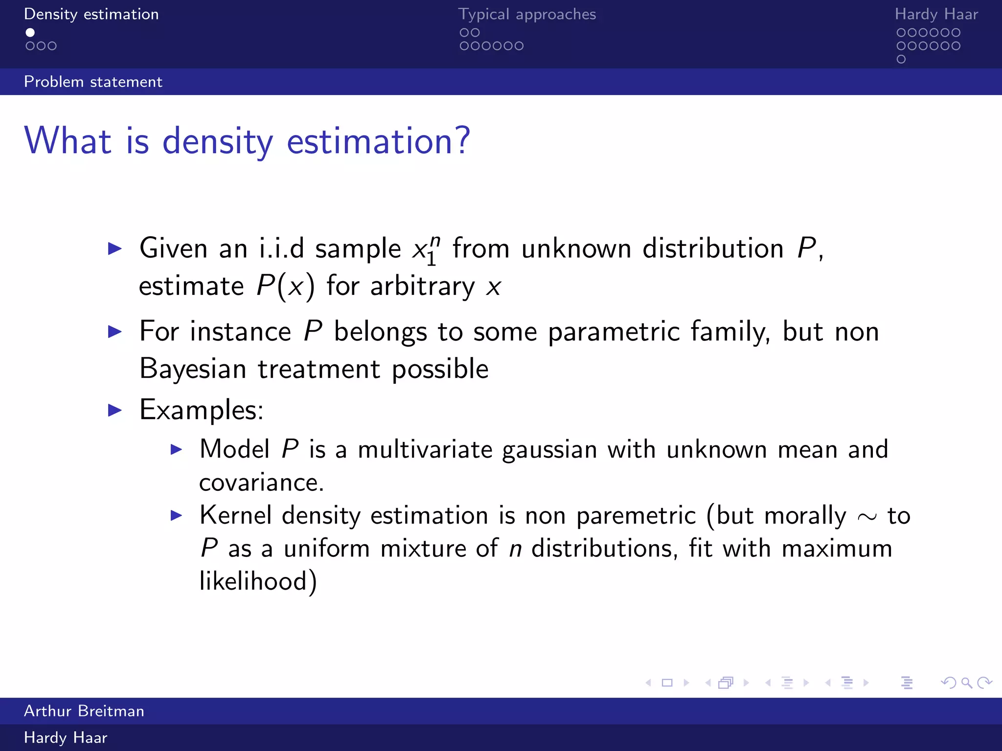
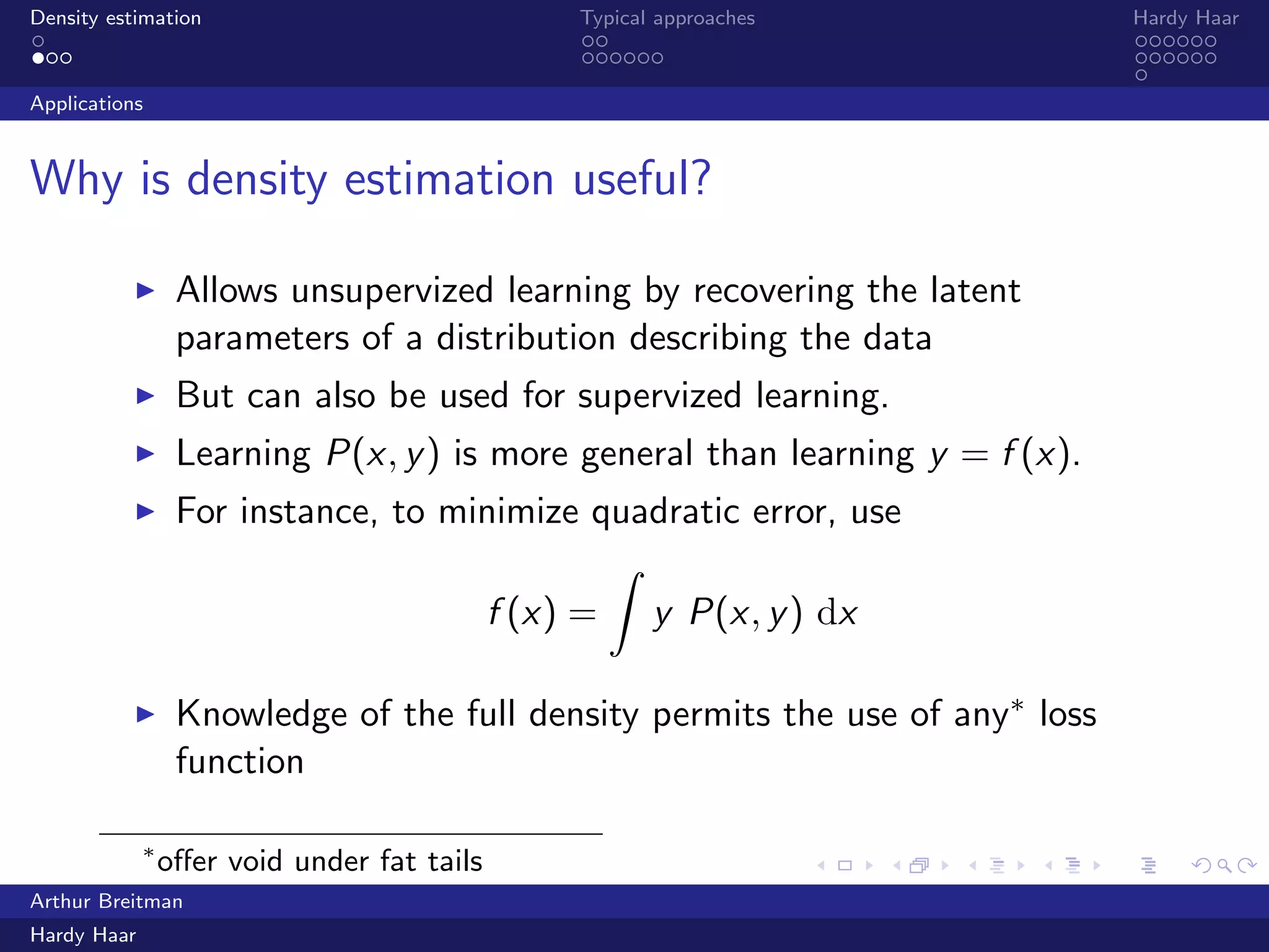
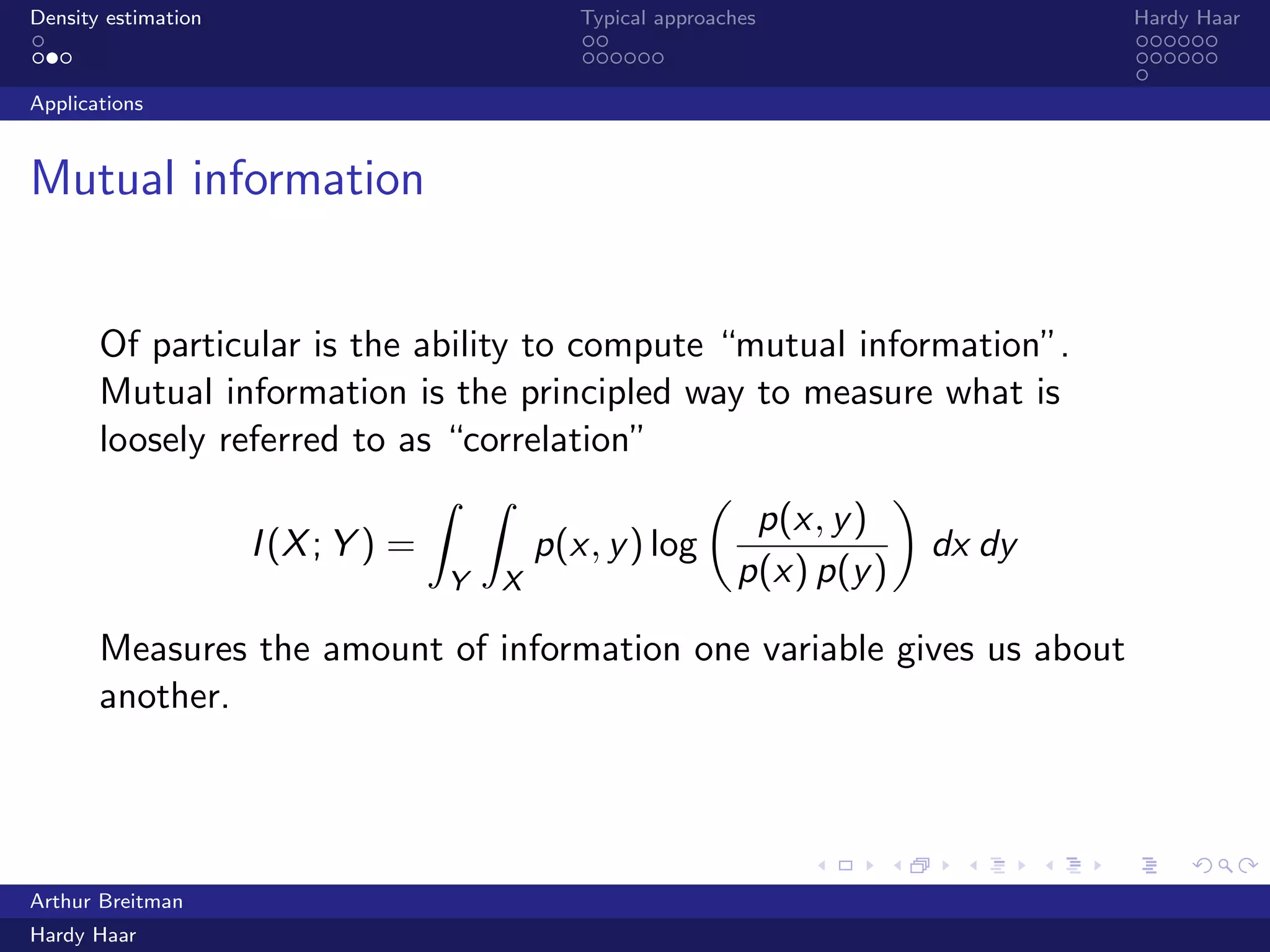
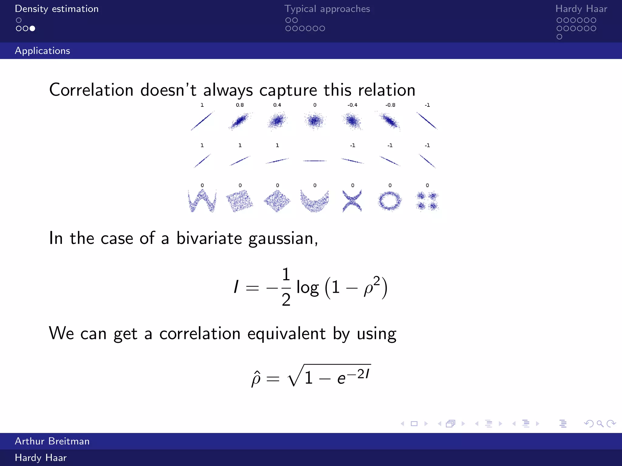
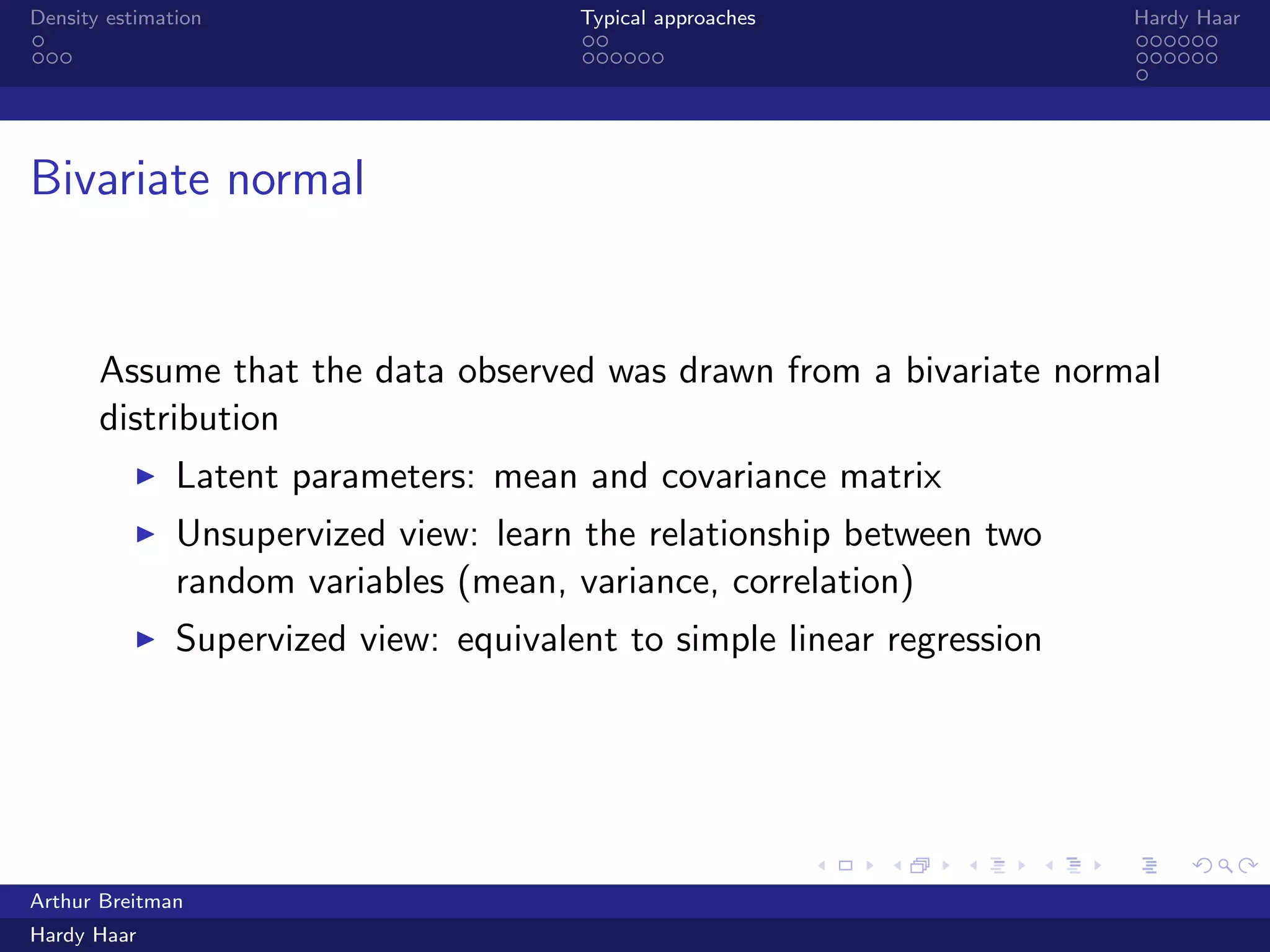
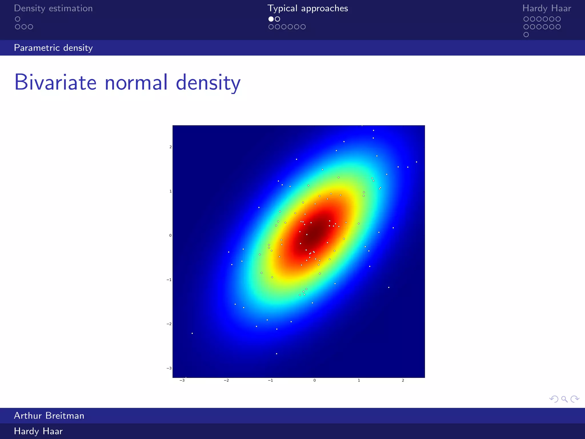
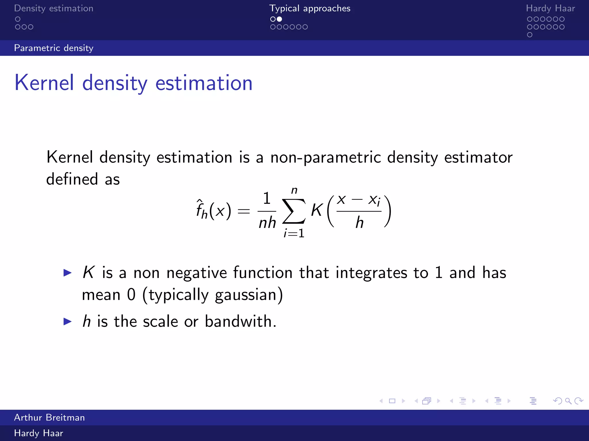
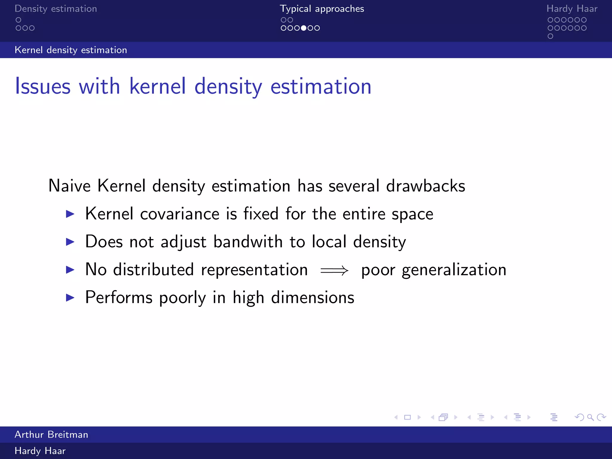
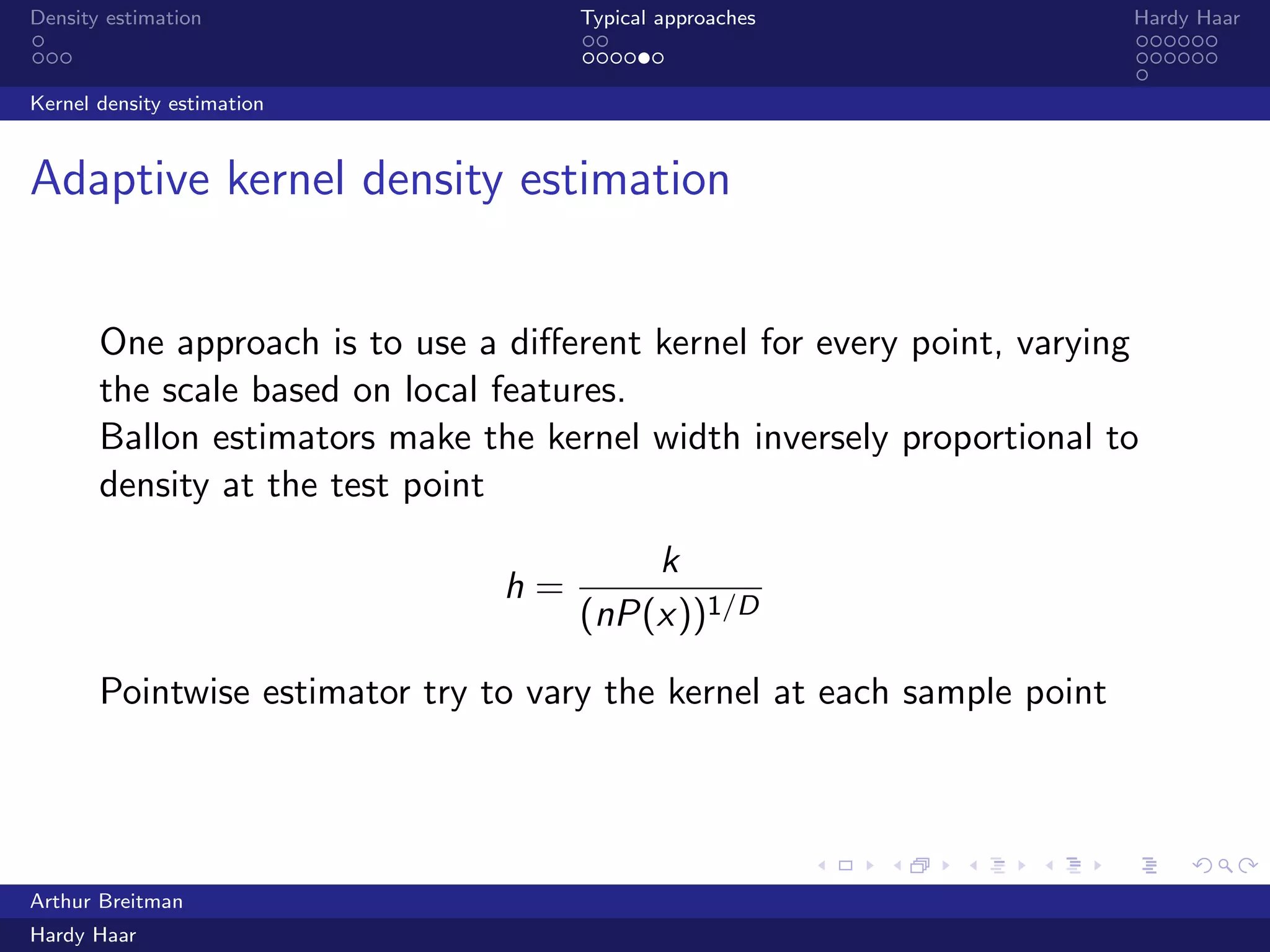
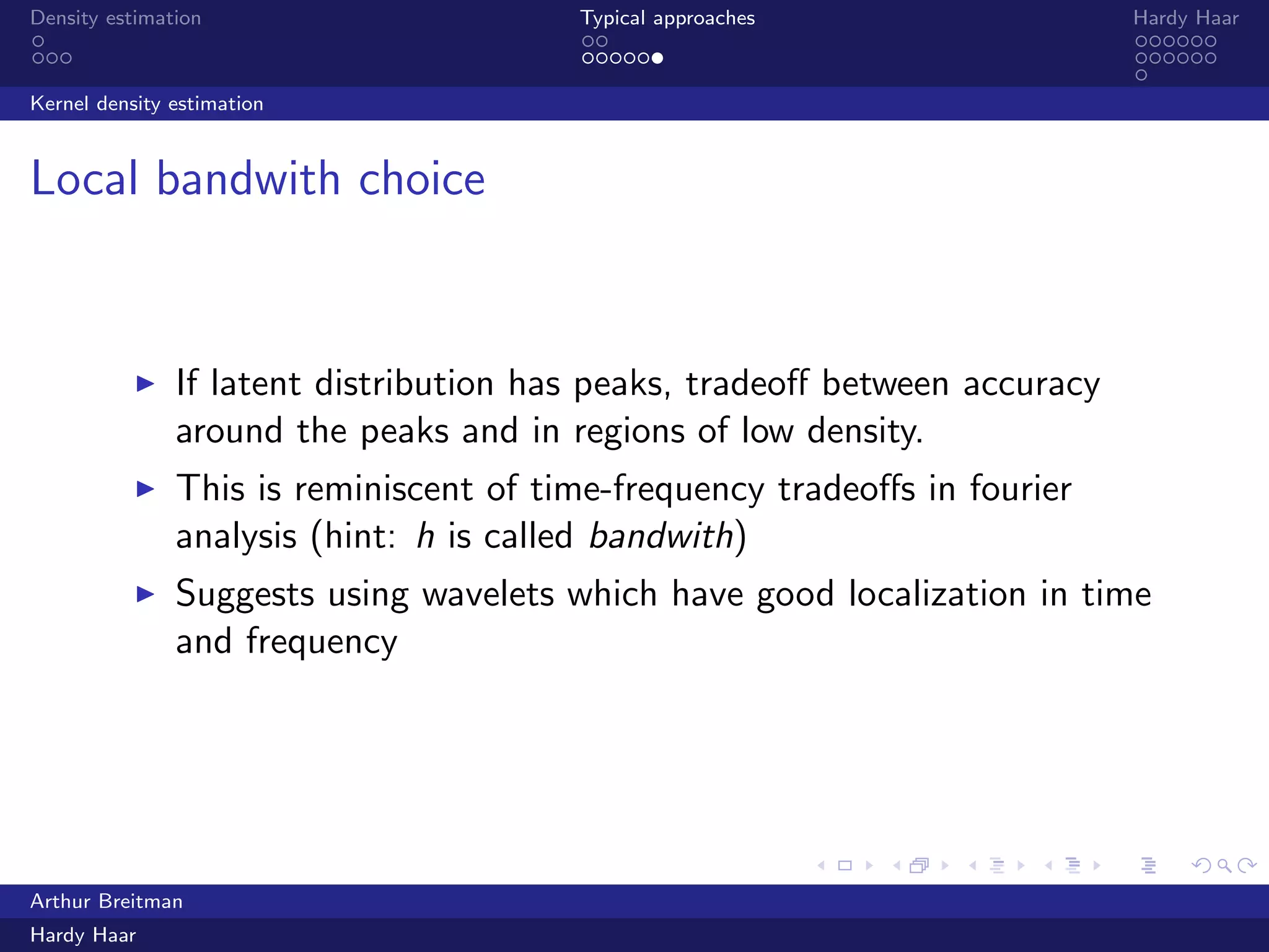
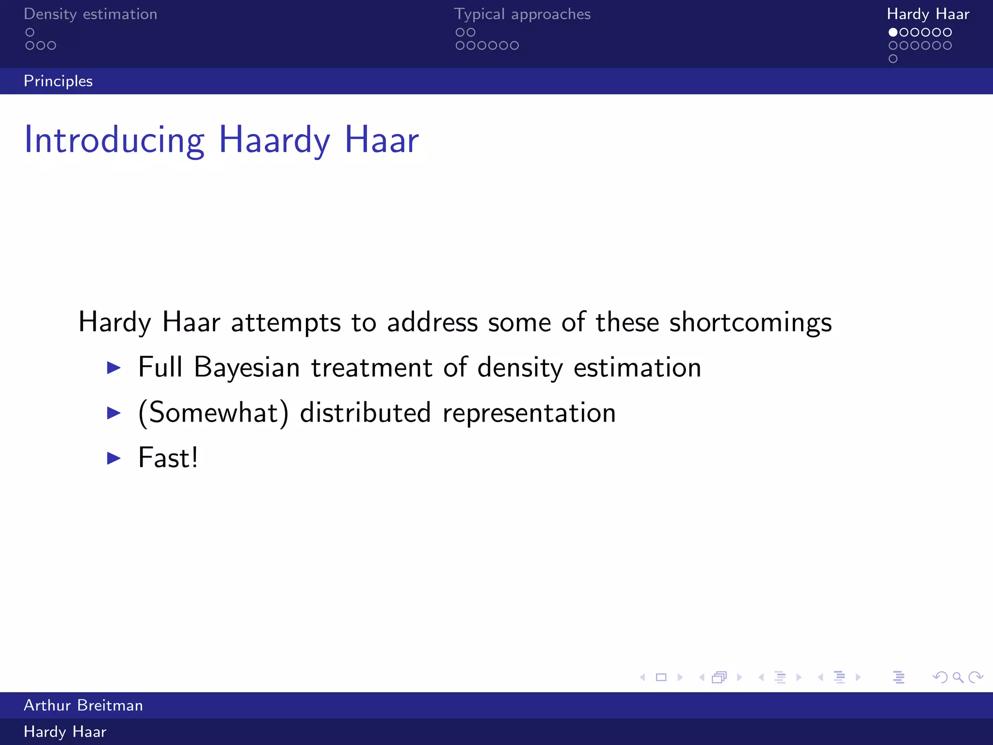
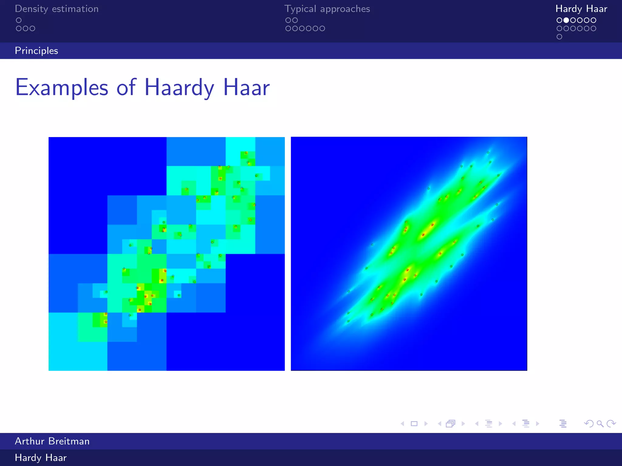
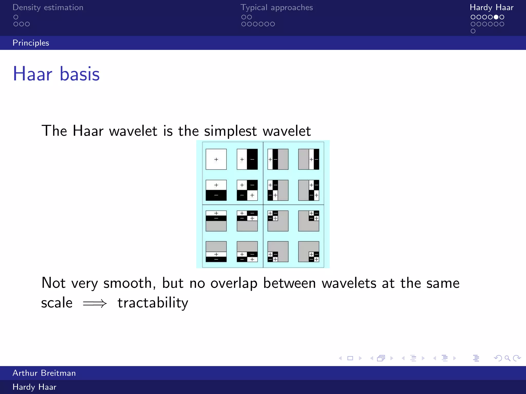
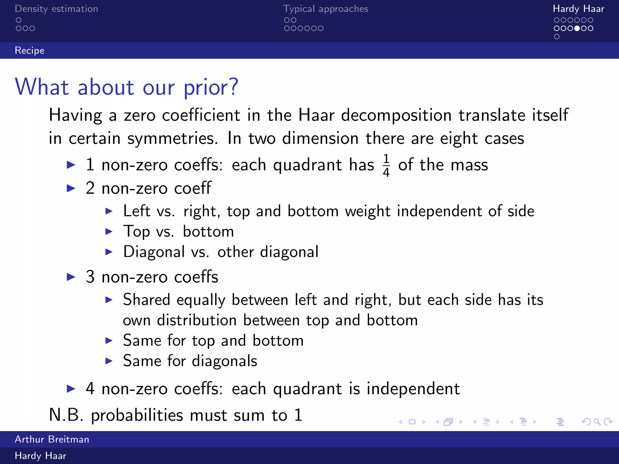
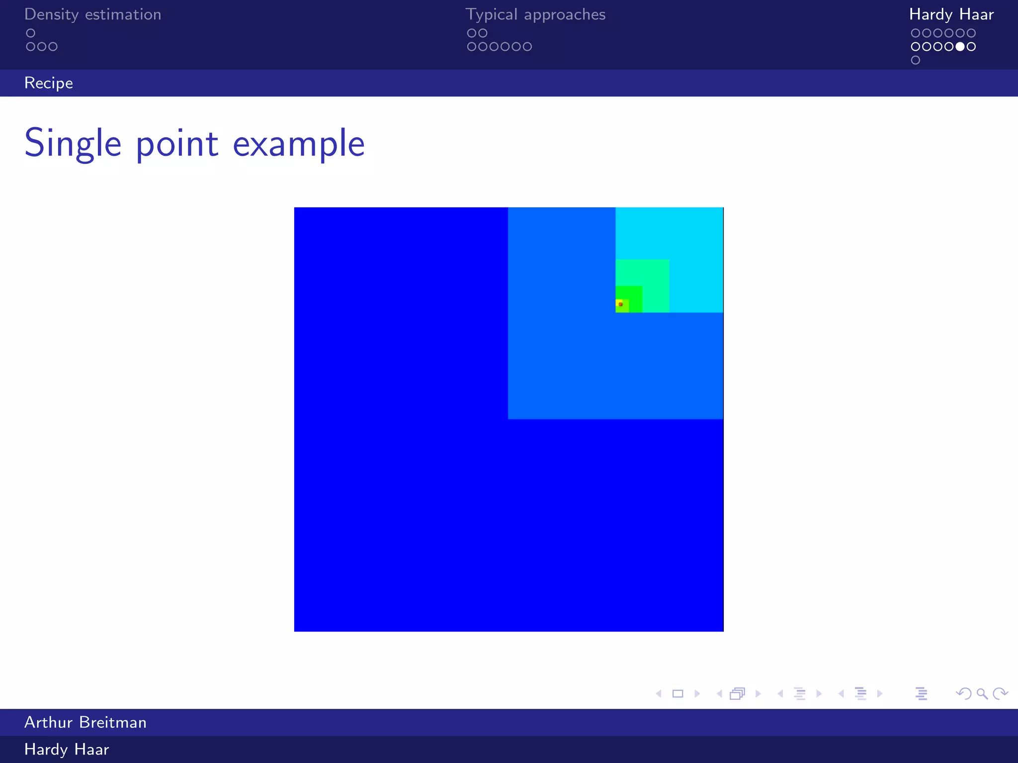
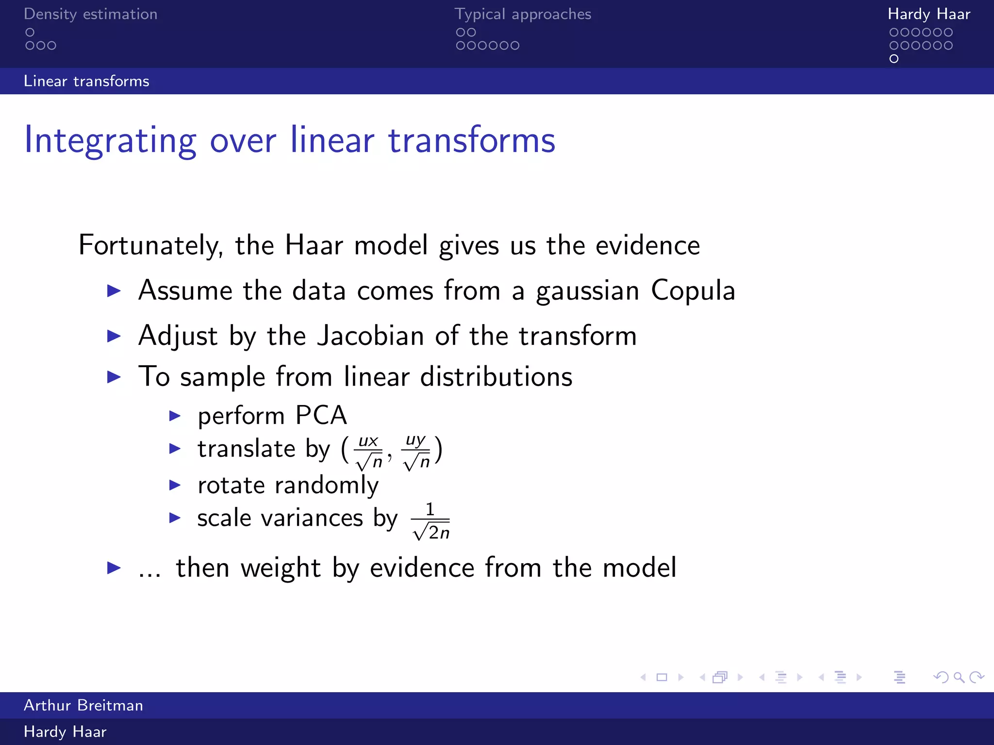
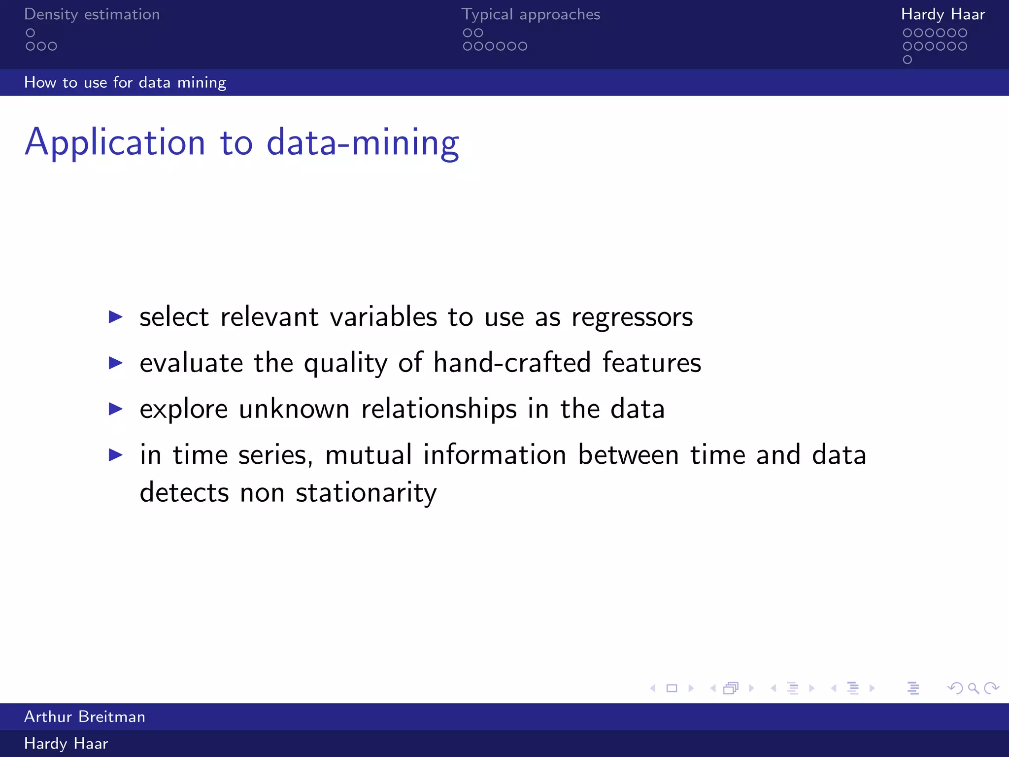
The document discusses density estimation, particularly through the Hardy Haar method, which addresses shortcomings in traditional approaches and employs a Bayesian treatment. It emphasizes applications in both unsupervised and supervised learning, with mutual information as a key concept for understanding relationships between variables. Additionally, it outlines the technical details of kernel density estimation and the use of wavelet decomposition for spatial coherence in prior distributions.

1. .
.
.
.
.
.
.
.
.
.
.
.
.
.
.
.
.
.
.
.
.
.
.
.
.
.
.
.
.
.
.
.
.
.
.
.
.
.
.
.
Density estimation Typical approaches Hardy Haar
Hardy Haar
Non-linear density estimation using a sparse Haar prior
Arthur Breitman
April 3, 2016
Arthur Breitman
Hardy Haar

2. .
.
.
.
.
.
.
.
.
.
.
.
.
.
.
.
.
.
.
.
.
.
.
.
.
.
.
.
.
.
.
.
.
.
.
.
.
.
.
.
Density estimation Typical approaches Hardy Haar
Table of contents
Density estimation
Problem statement
Applications
Typical approaches
Parametric density
Kernel density estimation
Hardy Haar
Principles
Recipe
Linear transforms
How to use for data mining
Arthur Breitman
Hardy Haar

3. .
.
.
.
.
.
.
.
.
.
.
.
.
.
.
.
.
.
.
.
.
.
.
.
.
.
.
.
.
.
.
.
.
.
.
.
.
.
.
.
Density estimation Typical approaches Hardy Haar
Problem statement
What is density estimation?
▶ Given an i.i.d sample xn
1 from unknown distribution P,
estimate P(x) for arbitrary x
▶ For instance P belongs to some parametric family, but non
Bayesian treatment possible
▶ Examples:
▶ Model P is a multivariate gaussian with unknown mean and
covariance.
▶ Kernel density estimation is non paremetric (but morally ∼ to
P as a uniform mixture of n distributions, fit with maximum
likelihood)
Arthur Breitman
Hardy Haar

4. .
.
.
.
.
.
.
.
.
.
.
.
.
.
.
.
.
.
.
.
.
.
.
.
.
.
.
.
.
.
.
.
.
.
.
.
.
.
.
.
Density estimation Typical approaches Hardy Haar
Applications
Why is density estimation useful?
▶ Allows unsupervized learning by recovering the latent
parameters of a distribution describing the data
▶ But can also be used for supervized learning.
▶ Learning P(x, y) is more general than learning y = f (x).
▶ For instance, to minimize quadratic error, use
f (x) =
∫
y P(x, y) dx
∫
P(x, y) dx
▶ Knowledge of the full density permits the use of any∗ loss
function
∗
offer void under fat tails
Arthur Breitman
Hardy Haar

5. .
.
.
.
.
.
.
.
.
.
.
.
.
.
.
.
.
.
.
.
.
.
.
.
.
.
.
.
.
.
.
.
.
.
.
.
.
.
.
.
Density estimation Typical approaches Hardy Haar
Applications
Mutual information
Of particular is the ability to compute “mutual information”.
Mutual information is the principled way to measure what is
loosely referred to as “correlation”
I(X; Y ) =
∫
Y
∫
X
p(x, y) log
(
p(x, y)
p(x) p(y)
)
dx dy
Measures the amount of information one variable gives us about
another.
Arthur Breitman
Hardy Haar

6. .
.
.
.
.
.
.
.
.
.
.
.
.
.
.
.
.
.
.
.
.
.
.
.
.
.
.
.
.
.
.
.
.
.
.
.
.
.
.
.
Density estimation Typical approaches Hardy Haar
Applications
Correlation doesn’t always capture this relation
In the case of a bivariate gaussian,
I = −
1
2
log
(
1 − ρ2
)
We can get a correlation equivalent by using
ˆρ =
√
1 − e−2I
Arthur Breitman
Hardy Haar

7. .
.
.
.
.
.
.
.
.
.
.
.
.
.
.
.
.
.
.
.
.
.
.
.
.
.
.
.
.
.
.
.
.
.
.
.
.
.
.
.
Density estimation Typical approaches Hardy Haar
Bivariate normal
Assume that the data observed was drawn from a bivariate normal
distribution
▶ Latent parameters: mean and covariance matrix
▶ Unsupervized view: learn the relationship between two
random variables (mean, variance, correlation)
▶ Supervized view: equivalent to simple linear regression
Arthur Breitman
Hardy Haar

8. .
.
.
.
.
.
.
.
.
.
.
.
.
.
.
.
.
.
.
.
.
.
.
.
.
.
.
.
.
.
.
.
.
.
.
.
.
.
.
.
Density estimation Typical approaches Hardy Haar
Parametric density
Bivariate normal density
Arthur Breitman
Hardy Haar

9. .
.
.
.
.
.
.
.
.
.
.
.
.
.
.
.
.
.
.
.
.
.
.
.
.
.
.
.
.
.
.
.
.
.
.
.
.
.
.
.
Density estimation Typical approaches Hardy Haar
Parametric density
Kernel density estimation
Kernel density estimation is a non-parametric density estimator
defined as
ˆfh(x) =
1
nh
n∑
i=1
K
(x − xi
h
)
▶ K is a non negative function that integrates to 1 and has
mean 0 (typically gaussian)
▶ h is the scale or bandwith.
Arthur Breitman
Hardy Haar

10. .
.
.
.
.
.
.
.
.
.
.
.
.
.
.
.
.
.
.
.
.
.
.
.
.
.
.
.
.
.
.
.
.
.
.
.
.
.
.
.
Density estimation Typical approaches Hardy Haar
Kernel density estimation
Gaussian kernel density estimation
Arthur Breitman
Hardy Haar

11. .
.
.
.
.
.
.
.
.
.
.
.
.
.
.
.
.
.
.
.
.
.
.
.
.
.
.
.
.
.
.
.
.
.
.
.
.
.
.
.
Density estimation Typical approaches Hardy Haar
Kernel density estimation
Bandwith selection
Picking h can be tricky
▶ h too small =⇒ overfit the data
▶ h too large =⇒ underfit the data
▶ There are rules of thumbs to pick h from variance of data and
number of points
▶ Can be picked by cross-validation
Arthur Breitman
Hardy Haar

12. .
.
.
.
.
.
.
.
.
.
.
.
.
.
.
.
.
.
.
.
.
.
.
.
.
.
.
.
.
.
.
.
.
.
.
.
.
.
.
.
Density estimation Typical approaches Hardy Haar
Kernel density estimation
Gaussian kernel density estimation
Under and over-fitting with different bandwiths (the correlation of
the kernel is estimated from the data)
Arthur Breitman
Hardy Haar

13. .
.
.
.
.
.
.
.
.
.
.
.
.
.
.
.
.
.
.
.
.
.
.
.
.
.
.
.
.
.
.
.
.
.
.
.
.
.
.
.
Density estimation Typical approaches Hardy Haar
Kernel density estimation
Issues with kernel density estimation
Naive Kernel density estimation has several drawbacks
▶ Kernel covariance is fixed for the entire space
▶ Does not adjust bandwith to local density
▶ No distributed representation =⇒ poor generalization
▶ Performs poorly in high dimensions
Arthur Breitman
Hardy Haar

14. .
.
.
.
.
.
.
.
.
.
.
.
.
.
.
.
.
.
.
.
.
.
.
.
.
.
.
.
.
.
.
.
.
.
.
.
.
.
.
.
Density estimation Typical approaches Hardy Haar
Kernel density estimation
Adaptive kernel density estimation
One approach is to use a different kernel for every point, varying
the scale based on local features.
Ballon estimators make the kernel width inversely proportional to
density at the test point
h =
k
(nP(x))1/D
Pointwise estimator try to vary the kernel at each sample point
Arthur Breitman
Hardy Haar

15. .
.
.
.
.
.
.
.
.
.
.
.
.
.
.
.
.
.
.
.
.
.
.
.
.
.
.
.
.
.
.
.
.
.
.
.
.
.
.
.
Density estimation Typical approaches Hardy Haar
Kernel density estimation
Local bandwith choice
▶ If latent distribution has peaks, tradeoff between accuracy
around the peaks and in regions of low density.
▶ This is reminiscent of time-frequency tradeoffs in fourier
analysis (hint: h is called bandwith)
▶ Suggests using wavelets which have good localization in time
and frequency
Arthur Breitman
Hardy Haar

16. .
.
.
.
.
.
.
.
.
.
.
.
.
.
.
.
.
.
.
.
.
.
.
.
.
.
.
.
.
.
.
.
.
.
.
.
.
.
.
.
Density estimation Typical approaches Hardy Haar
Principles
Introducing Haardy Haar
Hardy Haar attempts to address some of these shortcomings
▶ Full Bayesian treatment of density estimation
▶ (Somewhat) distributed representation
▶ Fast!
Arthur Breitman
Hardy Haar

17. .
.
.
.
.
.
.
.
.
.
.
.
.
.
.
.
.
.
.
.
.
.
.
.
.
.
.
.
.
.
.
.
.
.
.
.
.
.
.
.
Density estimation Typical approaches Hardy Haar
Principles
Examples of Haardy Haar
Arthur Breitman
Hardy Haar

18. .
.
.
.
.
.
.
.
.
.
.
.
.
.
.
.
.
.
.
.
.
.
.
.
.
.
.
.
.
.
.
.
.
.
.
.
.
.
.
.
Density estimation Typical approaches Hardy Haar
Principles
Goals
Coming up with a prior?
▶ In principle, any distribution whose support contains the
sample is potential.
▶ Some distributions are more likely than others, but why not
just take the empirical distribution?
▶ May work fine for integration problems for instance
▶ Doesn’t help with regression or to understand the data
▶ There should be some sort of spatial coherence to the
distribution
Arthur Breitman
Hardy Haar

19. .
.
.
.
.
.
.
.
.
.
.
.
.
.
.
.
.
.
.
.
.
.
.
.
.
.
.
.
.
.
.
.
.
.
.
.
.
.
.
.
Density estimation Typical approaches Hardy Haar
Principles
Sparse wavelet decomposition prior
To express the spatial coherence constraint, we take a L0 sparsity
prior over the coefficient of the decomposition of the PDF in a
suitable wavelet basis.
▶ This creates a coefficient ”budget” to describe the distribution
▶ Large scale wavelet describe coarse features of the distribution
▶ Sparse areas can be described with few coefficients
▶ Areas with a lot of sample points are described in more detail
▶ Closely adheres to the minimum description length principle
Arthur Breitman
Hardy Haar

20. .
.
.
.
.
.
.
.
.
.
.
.
.
.
.
.
.
.
.
.
.
.
.
.
.
.
.
.
.
.
.
.
.
.
.
.
.
.
.
.
Density estimation Typical approaches Hardy Haar
Principles
Haar basis
The Haar wavelet is the simplest wavelet
Not very smooth, but no overlap between wavelets at the same
scale =⇒ tractability
Arthur Breitman
Hardy Haar

21. .
.
.
.
.
.
.
.
.
.
.
.
.
.
.
.
.
.
.
.
.
.
.
.
.
.
.
.
.
.
.
.
.
.
.
.
.
.
.
.
Density estimation Typical approaches Hardy Haar
Principles
Model
▶ The minimum length principle suggests penalizing the log
likelihood of producing the sample with the number of non
zero coefficients.
▶ We can put a weight on the penalty, which will enforce more
or less sparsity
▶ We can “cheat” with an improper prior: use an infinite
number of coefficient, but favor models with many zeros
Arthur Breitman
Hardy Haar

22. .
.
.
.
.
.
.
.
.
.
.
.
.
.
.
.
.
.
.
.
.
.
.
.
.
.
.
.
.
.
.
.
.
.
.
.
.
.
.
.
Density estimation Typical approaches Hardy Haar
Recipe
Sampling
To sample from this distribution over distributions, conditional on
the observed sample, we interpret the data as generated by a
recursive generative model.
As n is held fixed, the number of datapoints in each orthant is
described by a multinomial distribution. We put a non-informative
dirichlet prior on the probabilities of each quadrant. This processus
is repeated for each orthant.
Arthur Breitman
Hardy Haar

23. .
.
.
.
.
.
.
.
.
.
.
.
.
.
.
.
.
.
.
.
.
.
.
.
.
.
.
.
.
.
.
.
.
.
.
.
.
.
.
.
Density estimation Typical approaches Hardy Haar
Recipe
Orthant tree
Place the data points in an orthant tree. The structure is built in
time O(n log n)
Arthur Breitman
Hardy Haar

24. .
.
.
.
.
.
.
.
.
.
.
.
.
.
.
.
.
.
.
.
.
.
.
.
.
.
.
.
.
.
.
.
.
.
.
.
.
.
.
.
Density estimation Typical approaches Hardy Haar
Recipe
Probabily of each orthant
Conditional on the number of datapoints falling in each orthant,
the distribution of the probability mass over each orthant is given
by the Dirichlet distribution:
Γ
(∑2d
i=1 ni
)
∏2d
i=1 Γ(1 + ni )
2d
∏
i=1
pni
i
d is the dimension of the space, thus there are 2d orthants.
Arthur Breitman
Hardy Haar

25. .
.
.
.
.
.
.
.
.
.
.
.
.
.
.
.
.
.
.
.
.
.
.
.
.
.
.
.
.
.
.
.
.
.
.
.
.
.
.
.
Density estimation Typical approaches Hardy Haar
Recipe
What about our prior?
Having a zero coefficient in the Haar decomposition translate itself
in certain symmetries. In two dimension there are eight cases
▶ 1 non-zero coeffs: each quadrant has 1
4 of the mass
▶ 2 non-zero coeff
▶ Left vs. right, top and bottom weight independent of side
▶ Top vs. bottom
▶ Diagonal vs. other diagonal
▶ 3 non-zero coeffs
▶ Shared equally between left and right, but each side has its
own distribution between top and bottom
▶ Same for top and bottom
▶ Same for diagonals
▶ 4 non-zero coeffs: each quadrant is independent
N.B. probabilities must sum to 1
Arthur Breitman
Hardy Haar

26. .
.
.
.
.
.
.
.
.
.
.
.
.
.
.
.
.
.
.
.
.
.
.
.
.
.
.
.
.
.
.
.
.
.
.
.
.
.
.
.
Density estimation Typical approaches Hardy Haar
Recipe
Single point example
Arthur Breitman
Hardy Haar

27. .
.
.
.
.
.
.
.
.
.
.
.
.
.
.
.
.
.
.
.
.
.
.
.
.
.
.
.
.
.
.
.
.
.
.
.
.
.
.
.
Density estimation Typical approaches Hardy Haar
Recipe
Marginalizing
▶ The distribution of weight over orthants is independent
between the “levels” of the tree
▶ We can marginalize to efficiently compute the mean density at
each point.
▶ The cost is then O(2d n log n)
Arthur Breitman
Hardy Haar

28. .
.
.
.
.
.
.
.
.
.
.
.
.
.
.
.
.
.
.
.
.
.
.
.
.
.
.
.
.
.
.
.
.
.
.
.
.
.
.
.
Density estimation Typical approaches Hardy Haar
Linear transforms
Orthant artifacts
▶ The model converges to the true distribution
▶ But the choice of orthants is arbitrary
▶ Introduces unnecessary variance
▶ We’d like to remove that sensitivity
Solution: integrate over all affine transforms of the data
Arthur Breitman
Hardy Haar

29. .
.
.
.
.
.
.
.
.
.
.
.
.
.
.
.
.
.
.
.
.
.
.
.
.
.
.
.
.
.
.
.
.
.
.
.
.
.
.
.
Density estimation Typical approaches Hardy Haar
Linear transforms
Integrating over linear transforms
Fortunately, the Haar model gives us the evidence
▶ Assume the data comes from a gaussian Copula
▶ Adjust by the Jacobian of the transform
▶ To sample from linear distributions
▶ perform PCA
▶ translate by ( ux√
n
, uy√
n
)
▶ rotate randomly
▶ scale variances by 1√
2n
▶ ... then weight by evidence from the model
Arthur Breitman
Hardy Haar

30. .
.
.
.
.
.
.
.
.
.
.
.
.
.
.
.
.
.
.
.
.
.
.
.
.
.
.
.
.
.
.
.
.
.
.
.
.
.
.
.
Density estimation Typical approaches Hardy Haar
How to use for data mining
Application to data-mining
▶ select relevant variables to use as regressors
▶ evaluate the quality of hand-crafted features
▶ explore unknown relationships in the data
▶ in time series, mutual information between time and data
detects non stationarity
Arthur Breitman
Hardy Haar