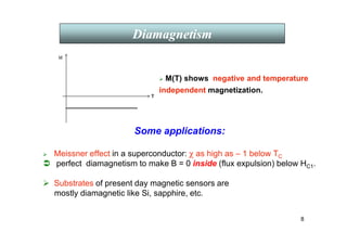
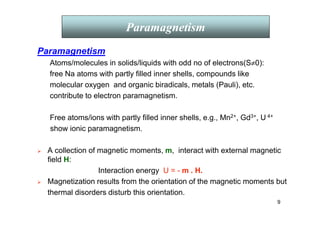
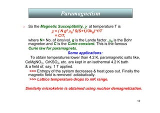
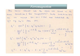
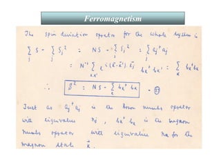
The document discusses the history and theories of magnetism, including topics such as diamagnetism, paramagnetism, and ferromagnetism, alongside their applications and underlying physical principles. It elaborates on various magnetic phenomena, including the Meissner effect in superconductors and the role of magnetic susceptibility in different materials. Additionally, the document covers quantum treatments of magnetic materials and significant contributions to the understanding of magnetism over time.


![6
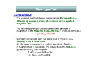
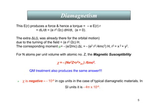
Diamagnetism
QM treatment
The Hamiltonian of a charged particle in a magnetic field B is
H = (p – eA/c)2/2m + eφ, A = vector pot, φ = scalar pot, valid for both
classical QM.
K.E. is not dependent on B, so it is unlikely that A enters H. But
p = pkin + pfield = mV + eA/c (Kittel, App. G, P: 654)
K.E. = (mV)2 /2m = (p – eA/c)2/2m, where B = ∇
∇
∇
∇ X A.
So, B-field-dependent part of H is ieh/4πmc[∇
∇
∇
∇. A+ A. ∇
∇
∇
∇ ] + e2 A2/2mc2.(1)](https://image.slidesharecdn.com/10344076-240909171948-1e3df6f2/85/NANO-MAGNETIC-MATERIALS-AND-APPLICATIONS-6-320.jpg)
![7
Diamagnetism
QM treatment
χ = LtH→0 (dM/dH) = - (Ne2Zr2av )/6mc2 independent of T.
M = - ∂E’/∂B = - (Ne2Zr2av )/6mc2 B for N atoms/volume with atomic no. Z.
Since B = H for non-magnetic materials
If B is uniform and II z-axis, AX = - ½ y B, AY = ½ x B, and AZ = 0.
So, (1) becomes H =(e/2mc) B [ih/2π(x ∂/∂y - y ∂/∂x)] + e2B2/8mc2(x2 + y2).
↓ ↓
LZ ⇒ Orbital PM; E’ = e2B2/12mc2 r2
by 1st order
perturbation theory.](https://image.slidesharecdn.com/10344076-240909171948-1e3df6f2/85/NANO-MAGNETIC-MATERIALS-AND-APPLICATIONS-7-320.jpg)
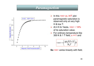
![11
In this m vs. H/T plot
paramagnetic saturation is
observed only at very high H low
T, i.e., x 1 when coth x →
→
→
→ 1 and
m →
→
→
→ NgµBS
At 4 K 1tesla, m ~ 14 % of its
saturation value.
For ordinary temperatures like 300
K 1 T field, x 1. Then coth x
→
→
→
→ 1/x + x/3 and so
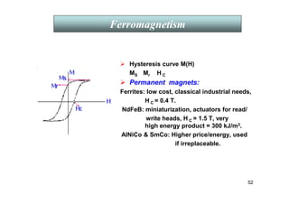
NgµB.
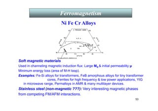
Paramagnetism
0 2 4 6 8 10
0.0
0.2
0.4
0.6
0.8
1.0
S=3/2 FOR Cr3++
Magnetic
Moments
Magnetic Field/Temperature(B/T)
H
T
k
S
S
g
m
B
B
+
→
3
)
1
(
µ
Thus m varies linearly with field.
m = Ngµ
µ
µ
µBS [coth X- 1/X] = L(X) = Langevin function when S →
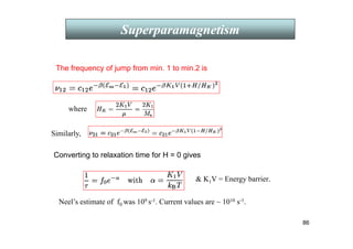
→
→
→ ∞
∞
∞
∞ with X = Sx.](https://image.slidesharecdn.com/10344076-240909171948-1e3df6f2/85/NANO-MAGNETIC-MATERIALS-AND-APPLICATIONS-11-320.jpg)
![13
Paramagnetism
Fascinating magnetic properties, also quite complex in nature:
Ce58: [Xe] 4f2 5d0 6s2, Ce3+ = [Xe] 4f1 5d0 since 6s2 and 4f1 removed
Yb70: [Xe] 4f14 5d0 6s2, Yb3+
= [Xe] 4f13 5d0 since 6s2 and 4f1 removed
Note: [Xe] = [Kr] 4d10 5s2 5p6.
In trivalent ions the outermost shells are identical 5s2 5p6 like neutral Xe.
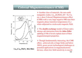
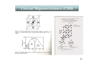
In La (just before RE) 4f is empty, Ce+++ has one 4f electron, this
number increases to 13 for Yb and 4f14 at Lu, the radii contracting from 1.11
Å (Ce) to 0.94 Å (Yb) → Lanthanide Contraction. The number of 4f
electrons compacted in the inner shell is what determines their magnetic
properties. The atoms have a (2J+1)-fold degenerate ground state which is
lifted by a magnetic field.
Rare–earth ions
In a Curie PM
=
( )
T
Np
T
C
T
g
J
NJ
B
B
B
κ
µ
κ
µ
χ β
3
3
1
2
2
2
2
=
=
+
= , p = effective Bohr Magnetron number
.
( )
[ ]
1
+
J
J
g
)
1
(
2
)
1
(
)
1
(
)
1
(
1
+
+
−
+
+
+
+
=
J
J
L
L
S
S
J
J
, g = Lande factor
‘p’ calculated from above for the +
3
RE ions using Hund’s rule agrees
very well with experimental values except for
3+
Eu +
3
Sm .](https://image.slidesharecdn.com/10344076-240909171948-1e3df6f2/85/NANO-MAGNETIC-MATERIALS-AND-APPLICATIONS-13-320.jpg)
![16
Paramagnetism
Explanation of 3rd rule:
Consequence of the sign of the spin-orbit interaction. For a single
electron, energy is lowest when S is antiparallel to L (L.S = - ve). But
the low energy pairs ml and ms are progressively used up as one adds
electrons to the shell. By PEP, when the shell is more than half full the
state of lowest energy necessarily has the S ║ L.
Examples of rule 3:
Ce3+ = [Xe] 4f1 5s2 5p6 since 6s2 and 4f1 removed. Similarly Pr3+ = [Xe]
4f2 5s2 5p6. Nd3+, Pm3+, Sm3+, Eu3+,Gd3+,Tb3+, Dy3+, Ho3+,Er3+ ,Tm3+,Yb3+
have 4f3 to 4f13. Take Ce3+: It has one 4f electron, an f electron has l = 3,
s = ½, 4f shell is less than half full (full shell has 14 electrons), by third
rule = J = L – S = L - 1/2 = 5/2.
J
s
L
1
2 +
2
/
5
2
F
+
3
Pr
Spectroscopic notation ⇒
⇒
⇒
⇒ [L = 0, 1, 2, 3, 4, 5, 6 are S, P, D, F, G, H, I].
has 2 ‘4f’ electrons: s = 1, l = 3. Both cannot have ml = 3 (PEP),
so max. L is not 6 but 5. J = L – S = 5 -1 = 4. ⇒
⇒
⇒
⇒ 3H4](https://image.slidesharecdn.com/10344076-240909171948-1e3df6f2/85/NANO-MAGNETIC-MATERIALS-AND-APPLICATIONS-16-320.jpg)
![17
Paramagnetism
Exactly ½ full 4f shell: : has 7 ’4f’ electrons; s = 7/2, L = 0, J = 7/2
+
3
Nd 2
/
9
4
I
+
3
Pm 4
5
I
has 3 ‘4f’ electrons: s = 3/2, L = 6 , J = 6 - 3/2 = 9/2 ⇒
has 4 ‘4f’ electrons: s = 2, L = 6, J = L - S = 4 ⇒
+
3
Gd
2
/
7
8
S
⇒
+
3
Ho ↑
↓ 8
5
I
4f shell is more than half full: has 10 ‘4f’ electrons: 7 will be ,
3 will be . S = 2, L = 6 [3 2 1 0 -1 -2 -3] ; J = 6 + 2 = 8 ⇒ and so on.
Note: 4f shell is well within the inner core (localized) surrounded by 5s2, 5p6, and
6s2 so almost unaffected by crystal field (CF).
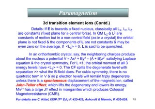
3d transition element ions
3d transition element ions, being in the outermost shell, are affected by strongly
inhomogeneous electric field, called the “crystal field” (CF) of neighboring ions in
a real crystal. L-S coupling breaks, so states are not specified by J. (2L + 1)
degenerate levels for the free ions may split by the CF and L is often quenched.
“p” calculated from J gives total disagreement with experiments.](https://image.slidesharecdn.com/10344076-240909171948-1e3df6f2/85/NANO-MAGNETIC-MATERIALS-AND-APPLICATIONS-17-320.jpg)
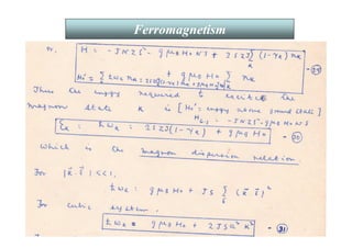
![21
Weiss proposed that:
i) Below TC spontaneously magnetized domains, randomly oriented
give M ~ 0 at H=0. A small H0 produces domain growth with M || H0.
ii) A very strong “molecular field”, HE of unknown origin aligns the
atomic moments within a domain.
Taking alignment energy ~ thermal energy below Tc,
For Fe: HE = kBTC / µ ~ 107 gauss ~ 103 T !!!
Ed-d ~ [µ1. µ2 - (µ1.r12) (µ2.r12)]/4πε0r3.
Classical dipole-dipole interaction gives a field of ~ 0.1 T only
is anisotropic but ferromagnetic anisotropy is only a second
order effect. So ???
Weiss postulated that HE = λM, where λ is the molecular field
parameter and M is the saturation magnetization.
Ferromagnetism
Weiss’ “molecular field” theory](https://image.slidesharecdn.com/10344076-240909171948-1e3df6f2/85/NANO-MAGNETIC-MATERIALS-AND-APPLICATIONS-21-320.jpg)
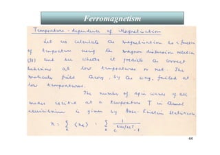
![22
Curie-Weiss law
Curie theory of paramagnetism gave
M = [( N g2 µB
2 S(S+1)/3kB)*1/T]*H
= (C/T)*H.
Replacing H by H0 + λM we get
M = CH0/(T-Cλ)
∴
∴
∴
∴ χ
χ
χ
χ = C/(T-T*C ),
where T*C = Cλ = paramagnetic Curie
temperature.
Putting g ~ 2, S = 1, M = 1700 emu/g
one gets λ = 5000 HE = 103 T for Fe.
This theory fails to explain χ (T) for
T T*C .
Ferromagnetism](https://image.slidesharecdn.com/10344076-240909171948-1e3df6f2/85/NANO-MAGNETIC-MATERIALS-AND-APPLICATIONS-22-320.jpg)
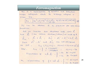
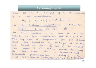
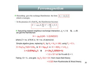
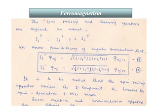
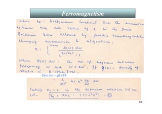
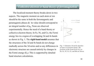
![26
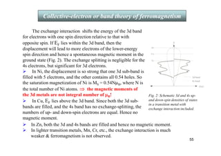
Heisenberg’s Theory (Exchange effect)
2
1
2
1
2
2
*
1
*
)
(
)
(
)
(
)
( r
d
r
d
r
u
r
u
r
r
e
r
u
r
u
J i
j
j
i
j
i
ij
r
r
r
r
r
r
r
r
∫ −
=
Ferromagnetism
Heisenberg found the origin of Weiss’ “molecular field” in the “quantum
mechanical exchange effect”, which is basically electrical in nature.
Electron spins on the same or neighboring atoms tend to be coupled by
the exchange effect – a consequence of Pauli’s Exclusion Principle. If ui
and uj are the two wave-functions into which we “put 2 electrons”, there
are two types of states that we can construct according to their having
antiparallel or parallel spins. These are
Ψ (r1, r2) =1/√2 [ui (r1) uj (r2) ± uj (r1) ui (r2)] where
± correspond to space symmetric/antisymmetric (spin singlet, S = 0/spin
triplet, S = 1) states.
Singlet: spin anisymmetric: S = 0: (↑↓ - ↓↑)/ √2 , m = 0.
Triplet: spin symmetric: S = 1: ↑↑ m = 1; ↓↓ m = -1;
(↑↓ + ↓↑)/ √2 , m = 0.
Also, if you exchange the electrons between the two states, i.e.,
interchange r1 and r2, Ψ(-) changes sign but Ψ(+) remains the same. If
the two electrons have the same spin(║), they cannot occupy the same
r. Thus Ψ(-) = 0 if r1 = r2. Now if you calculate the average of the
Coulomb energy e2/│r12 │in these two states we find them different by
which is the “exchange integral”.](https://image.slidesharecdn.com/10344076-240909171948-1e3df6f2/85/NANO-MAGNETIC-MATERIALS-AND-APPLICATIONS-26-320.jpg)
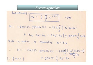
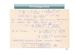
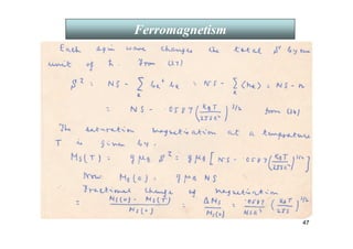
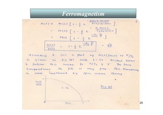
![51
Using the spin-wave dispersion relation for a cubic
system
(h/2π)ωk = gµBH0 + 2Jsa2k2,
one calculates the number of magnons, n in thermal
equilibrium at temperature T to be proportional to T3/2
and hence
M(T) = M(0) [1+ AZ{3/2, Tg/T} T3/2 + BZ {5/2,Tg/T}T5/2].
This is the famous Bloch’s T3/2 .
Similarly specific heat contribution of magnons is also
~ T3/2.
Both are in very good agreement with experiments.
Ferromagnetism
Spontaneous magnetization,
MS of a ferromagnet as a
function of reduced
temperature T/TC.
Bloch’s T3/2 law holds only
for T/TC 1.
Ferromagnetism
Ferromagnetism
Summary of spin-wave theory](https://image.slidesharecdn.com/10344076-240909171948-1e3df6f2/85/NANO-MAGNETIC-MATERIALS-AND-APPLICATIONS-51-320.jpg)
![62
• RKKY interaction ~ cos(2kf r)/(2kf r)3 .
• Established by experiments on light scattering by spin waves.
[ P. Grünberg et al., Phys. Rev. Lett. 57, 2442(1986).]
At high fields the spins align
with the field (saturating at Hsat)
and the resistance is reduced.
Magnetoresistance is negative!
At low fields the interlayer antiferromgnetic
coupling causes the spins in adjacent layers
to be antiparallel and the resistance is high
III. Giant Magnetoresistance (GMR)
Fe-Cr is a lattice matched pair : Exchange coupling of ferromagnetic Fe
layers through Cr spacers gives rise to a negative giant magnetoresistance
(GMR) with the application of a magnetic field.
Introduction
Magnetoresistance](https://image.slidesharecdn.com/10344076-240909171948-1e3df6f2/85/NANO-MAGNETIC-MATERIALS-AND-APPLICATIONS-62-320.jpg)
![63
Fe-Cr
Magnetoresistance is defined by
.
%
100
)
,
0
(
)
,
0
(
)
,
(
×
−
=
T
T
T
H
MR
ρ
ρ
ρ
(1)
Giant Magnetoresistance (GMR)
Giant Magnetoresistance (GMR)
Bulk scattering Interface scattering
[ Magnetic Multilayers and Giant Magnetoresistance, Ed. by Uwe Hartmann,
Springer Series in Surface Sciences, Vol. 37, Berlin (1999).]](https://image.slidesharecdn.com/10344076-240909171948-1e3df6f2/85/NANO-MAGNETIC-MATERIALS-AND-APPLICATIONS-63-320.jpg)
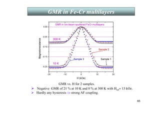
![64
Sample structure
Cr(t Å)
30 bi-layers
of Fe/Cr
Sample details
Si/Cr(50Å)/[Fe(20Å)/Cr(tÅ)]×30/Cr((50-t)Å)
Varying Cr thickness t = 6, 8, 10, 12, and 14 Å
Cr ( 50-t )Å
Cr 50 Å
Si Substrate
Fe/Cr multilayers prepared by ion-beam sputtering technique.
Ar and Xe ions were used.
Beam current 20 mA /30 mA and energy 900eV/1100eV.
Fe(20 Å)
bi-layer
GMR in Fe-Cr multilayers](https://image.slidesharecdn.com/10344076-240909171948-1e3df6f2/85/NANO-MAGNETIC-MATERIALS-AND-APPLICATIONS-64-320.jpg)
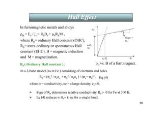
![67
RS ( Extra-ordinary or spontaneous Hall constant ) :
a) Classical Smit asymmetric scattering(AS).
b) Non-classical transport (side-jump).
Boltzmann Eq. is correct to the lowest order in («1) (τ = relaxation time),
true for pure metals and dilute alloys at low temperatures.
RS caused by AS of electrons by impurities in the presence of spin-orbit
interaction in a ferromagnet .
Boltzmann Eq.
a) Classical Smit asymmetric scattering (AS)
,
where [s] = relaxation frequency tensor ~ impurity concentration.
Off-diagonal elements describe AS proportional to M.
Diagonal elements give Ohmic ρ.
Boundary condition: jy= 0 ⇒
⇒
⇒
⇒ ρH and ρ.
RS = a ρ.
[L. Berger, Phys. Rev. 177, 790(1969).]
F
E
τ
h
[ ]j
s
e
m
B
j
E
en
dt
p
d r
r
r
r
r
−
×
+
=
Introduction (theory)
Hall Effect](https://image.slidesharecdn.com/10344076-240909171948-1e3df6f2/85/NANO-MAGNETIC-MATERIALS-AND-APPLICATIONS-67-320.jpg)
![68
b) Non-classical transport (side-jump mechanism)
is not small ⇒ Concentrated and disordered alloys, high temperatures.
[R. Karplus and J. M. Luttinger, Phys. Rev. 95, 1154 (1954).]
Calculation: Free electron plane wave (e i kx ) is scattered by a short-range
square well impurity potential
with V(r) = 0 for r R V(r) = V0 for r R. Using Born approx. one finds
a side-wise displacement of the wave-packet ∆y ~ 0.1-0.2 nm (side-jump).
F
E
τ
h
Z
Z S
L
r
V
r
c
m
r
V
m
H
∂
∂
+
+
∇
−
=
1
2
1
)
(
2 2
2
2
2
h
Transport theory for arbitrary ωcτ = e B τ / m, ωc= cyclotron frequency gives
ρH = R0Bz + µ0RSM , where RS = b ρ2.
Combining Eqs.(3) (4) for the most general case one gets
RS = a ρ + b ρ2 .
[L. Berger and G. Bergmann , in the Hall effect and its applications, edited by C. L.
Chien and C. R. Westgate (Plenum, New York , 1980), p.55 and references therein.]
Introduction (theory)
Hall Effect](https://image.slidesharecdn.com/10344076-240909171948-1e3df6f2/85/NANO-MAGNETIC-MATERIALS-AND-APPLICATIONS-68-320.jpg)
![t = 0 t = 0
t « 0
t » 0
t « 0
Y
Y
t » 0
δ
y
S
a) b)
Skew scattering Side jump scattering
[L. Berger and G. Bergmann , in the Hall effect and its applications, edited by C. L. Chien
and C. R. Westgate (Plenum, New York , 1980), p.55 and references therein.]
Hall Effect
69](https://image.slidesharecdn.com/10344076-240909171948-1e3df6f2/85/NANO-MAGNETIC-MATERIALS-AND-APPLICATIONS-69-320.jpg)
![Hall effect in GMR multilayers
All the theories discussed earlier are valid for homogeneous ferromagnets.
Scaling law is valid only in the local limit; the mean free path λ « d, the
layer thickness. It is invalid in the long mean free path limit; λ » d.
Zhang had shown the failure of scaling law in composite magnetic-
nonmagnetic systems:
The standard boundary condition used for calculating ρH, jy(z) = 0, is not
valid here for all z, but jy(z), integrated over z, is zero.
The two-point local Hall conductivity is given by
σyx (z, z') ∝ (m λSO MZ σCIP (z, z'))/τ(z), (3)
where σCIP (z, z') is the CIP two-point Ohmic conductivity.
To get σyx, integrate σyx (z, z') over z and z' and sum over the
spin variables.
[S. Zhang , Phys. Rev. B 51 , 3632(1995).]
Theory of Hall effect in inhomogeneous ferromagnets
Theory of Hall effect in inhomogeneous ferromagnets
70](https://image.slidesharecdn.com/10344076-240909171948-1e3df6f2/85/NANO-MAGNETIC-MATERIALS-AND-APPLICATIONS-70-320.jpg)
![0 1 2 3 4 5 6 7
0.0
1.5
3.0
4.5
6.0
7.5
9.0
Peak position
T = 300K
T = 4.2K
F8 (30L)
Hall
Resistivity
(10
-9
Ω
m)
Field (tesla)
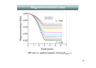
Hall resistivity (ρH) vs. applied magnetic field (µ0Happlied ).
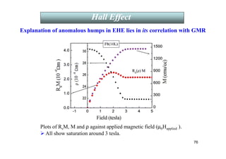
Q 3. Why do the humps appear in the EHE just before the
saturation field in these GMR systems?
Hall Effect data
Hall Effect data
In Hall geometry B = µ0[Happlied+ (1-N) M], N=demagnetization factor.
74](https://image.slidesharecdn.com/10344076-240909171948-1e3df6f2/85/NANO-MAGNETIC-MATERIALS-AND-APPLICATIONS-74-320.jpg)
![5.6 5.8 6.0 6.2
0.0
0.3
0.6
0.9
1.2
1.5
F10(30L)
n = 3.45 ± 0.11
F10(10L)
n = 3.07 ± 0.04
Rs
~ ρ
n
ln
R
s
ln ρ (at B = 0)
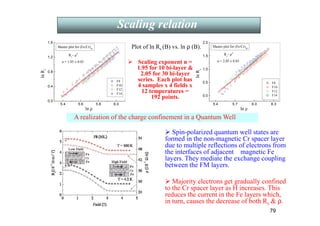
Plot of ln Rs vs. ln ρ (ρ being the resistivity at B = 0).
Q 4. Why has the scaling law failed ?
Scaling relation
Scaling relation
Fits to RS = a ρ + b ρn with a = 0 yield n much larger than 2 as found earlier in
Fe-Cr, Co-Cu, and Co-Ag films. [Y. Aoki et al., J. Magn. Magn. Mater. 126 , 448
(1993); T. Lucin´ski et al., J. Magn. Magn. Mater. 160 , 347 (1996); V. Korenivski et
al., Phys. Rev. B 53 , R 11 938 (1996).]
The exponent is larger for samples having higher GMR !!!
77](https://image.slidesharecdn.com/10344076-240909171948-1e3df6f2/85/NANO-MAGNETIC-MATERIALS-AND-APPLICATIONS-77-320.jpg)
![81
Nano-scale magnetism: Magnetic properties like Tc(Curie
temperature), Ms(Saturation magnetization), and Hc (Coercive
field) change as the size reduces to 100 nm, due to higher
surface /volume ratio.
(A) (B) (C)
(A) Specific magnetization vs. temperature at 1.2 tesla.
(B) Specific magnetization vs. average diameter of Ni particles.
(C) Coercivity vs. average diameter of Ni particles.
[You-wei Du, Ming-xiang Xu, Jian Wu, Ying-bing Shi, and Huai-xian Lu,
J. Appl. Phys. 70, 5903 (1991).]
Electrical transport properties are seriously affected by grain
boundary scattering.
Nano-magnetism](https://image.slidesharecdn.com/10344076-240909171948-1e3df6f2/85/NANO-MAGNETIC-MATERIALS-AND-APPLICATIONS-81-320.jpg)
![88
The final form of m along the direction of H comes out to be
where BS (x) is the Brillouin function
Paramagnetism
=
T
k
SH
g
SB
g
m
B
B
S
B
µ
µ
−
+
+
=
S
x
S
S
x
S
S
S
2
coth
2
1
2
)
1
2
(
coth
2
1
2
where S is the spin of the ion.
m = g µ
µ
µ
µB [coth x- 1/x] = L(x) = Langevin function when S →
→
→
→ ∞
∞
∞
∞ .](https://image.slidesharecdn.com/10344076-240909171948-1e3df6f2/85/NANO-MAGNETIC-MATERIALS-AND-APPLICATIONS-88-320.jpg)
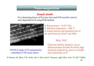
![93
A cross-sectional STEM-Z image
Ni [220] || TiN[002]
Ni[110] || TiN[110]
Ni [002] || TiN[002]
Ni[110] || TiN[110]
Single layer epitaxial Ni nano dots on TiN/Si(100) template
Ni separation ≈ 10 nm
Triangular morphology
with 17 nm base and
9 nm height
Some have rectangular
morphology.
Thickness of TiN = 6×32 nm.
Ni particles grow epitaxially on TiN acting as a template which also
grows epitaxially on Si.
Ni-nano/TiN is an ideal system for studying electrical transport in magnetic
nano particles due to epitaxial growth and conducting nature of TiN .
Nano-magnetism](https://image.slidesharecdn.com/10344076-240909171948-1e3df6f2/85/NANO-MAGNETIC-MATERIALS-AND-APPLICATIONS-93-320.jpg)
![94
Hall Effect
0 1 2 3 4 5
0
1x10
-10
2x10
-10
3x10
-10
4x10
-10
5x10
-10
6x10
-10
T=25K
T = 300K
Hall effect
Ni-Nano/TiN
Hall effect
Pure Ni-bulk
11K
35K
60K
85K
105K
115K
135K
160K
185K
210K
235K
260K
290K
T=290K
T=11K
Hall
Resistivity
(-
ρ
H
)(ohm-m)
Field (tesla)
Hall resistivity (ρH) vs. applied magnetic field (µ0Happlied ).
ρH is negative at all temperatures from 11 to 290 K.
In Hall geometry B = µ0[Happlied+ (1-N) M], N=demagnetization factor.
So, ρH = Ro µ0 Happlied + RS µ0 M,
Nano-magnetism](https://image.slidesharecdn.com/10344076-240909171948-1e3df6f2/85/NANO-MAGNETIC-MATERIALS-AND-APPLICATIONS-94-320.jpg)
![95
-3000 -2000 -1000 0 1000 2000 3000
-1.8
-1.2
-0.6
0.0
0.6
1.2
1.8
0.20
0.25
0.30
0.35
0 100 200 300
50
100
150
200
250
Hc
H
C
(Oe)
T (K)
M
r
(10
-4
emu)
Mr
M
(10
-
4
emu)
Field (tesla)
(10 K)
(100 K)
(300 K)
Magnetization vs. applied field at 10, 100 and 300 K.
Inset: Coercivity remanent magnetization vs. T.
Magnetization
Nano-magnetism
[P. Khatua, T. K. Nath, and A. K. Majumdar, Phys. Rev. B 73, 064408 (2006).]](https://image.slidesharecdn.com/10344076-240909171948-1e3df6f2/85/NANO-MAGNETIC-MATERIALS-AND-APPLICATIONS-95-320.jpg)