24CSK34-OPTIMIZATION TECHNIQUES
MODULE-1-OPTIMIZATION TECHNIQUESAND LINEAR PROGRAMMING
INTRODUCTION:
• Evolution
• Definitions and Applications of Optimization Techniques,
• Models used in OT
• Characteristics and phases of OT
• Computer software for OT
LINEAR PROGRAMMING:
• Mathematical formulation of Linear Programming Problems,
• Graphical solution methods,
• The Algebraic Method.
4.
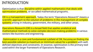
INTRODUCTION
Optimization is thatdiscipline within applied mathematics that deals with
optimization problems, or so-called mathematical programs.
OR is a management approach. Today the term “Operations Research” means a
scientific approach to the solution of problems in the management of complex
systems arising in industry, government, the military, and other areas.
Operations Research (OR) is a broad field that applies analytical and
mathematical methods to solve complex decision-making problems in various
sectors like business and engineering.
Optimization is a core and fundamental subfield of OR, focusing on finding the
best possible solution (a maximum or minimum value) for a problem with well-
defined objectives and constraints. In essence, optimization is the primary tool
used within the larger framework of Operations Research.
5.
INTRODUCTION
• Optimization techniquesare methods to find the best
possible solution to a problem by maximizing or minimizing
a function under certain constraints.
• These techniques are broadly categorized into classical
methods (like linear programming), numerical methods
(such as gradient descent), and evolutionary algorithms
(like genetic algorithms).
• The choice of technique depends on the nature of the
problem, such as whether it involves continuous or discrete
variables and if the functions are differentiable.
6.
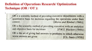
Definition of OperationsResearch/ Optimization
Technique (OR / OT ):
Operations Research (OR/ OT) is a scientific
approach to decision-making that applies
mathematical, statistical, and analytical methods
to find the best possible solution to complex real-
world problems.
It is often used to optimize resources (time, money,
manpower, machines, etc.) and improve efficiency
in industries, business, government, and
engineering.
OR / OT helps in choosing the best option among many
alternatives using quantitative analysis.
EVOLUTION OF OR
•The term "Operations Research" (often abbreviated as OR)
was first coined in 1940 by McClosky and Treffhen in the UK.
• It emerged from the need to solve complex military
problems during World War II, with teams of scientists from
various disciplines working together to analyze operations
and suggest improvements.
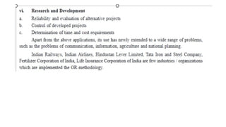
• The field has since expanded to encompass a wide range of
applications in various industries.
10.
EVOLUTION OF OR
•The evolution of OR can be traced through four distinct phases:
• The early years (1930s-1950s):
• This was the period when OR was first developed and applied to military problems. During this time,
OR practitioners developed many of the basic tools and techniques that are still used today, such as
linear programming, queuing theory, and game theory.
• The growth years (1950s-1970s):
• OR began to be applied to a wider range of problems in the 1950s and 1960s. This was due in part
to the development of new computing technologies, which made it possible to solve more complex
problems. During this time, OR also began to be taught in universities, which helped to increase the
number of OR practitioners.
• The maturity years (1970s-1990s):
• OR reached a level of maturity in the 1970s and 1980s. During this time, OR practitioners focused on
developing more specialized tools and techniques for solving specific problems. OR also began to
be used in a wider range of industries, including healthcare, transportation, and manufacturing.
• The modern era (1990s-present):
• OR has continued to evolve in the modern era. During this time, OR practitioners have made use of
new technologies, such as artificial intelligence and big data, to solve even more complex problems.
OR has also become more internationalized, with practitioners working in countries all over the
world.
11.
The objective ofOperations Research /
Optimization Techniques
• The objective of Operations Research / Optimization
Techniques
• The objective of Operations Research is to provide a
scientific basis to the decision maker for solving the
problems involving the interaction of various components of
an organization by employing a team of scientists from
various disciplines, all working together for finding a
solution which is in the best interest of the organisaton as a
whole.
• The best solution thus obtained is known as optimal
decision"
Why Study Operations Research (OR)?
Operations Research is studied because it improves decision-
making and optimizes the use of resources. In today’s world,
where businesses and organizations face complex problems, OR
provides a scientific and systematic way to handle them.
12.
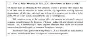
Why Study OperationsResearch? (Importance of OR)
Managerial Perspective
Engineers and managers must learn OR techniques to improve their decision-making ability.
OR bridges the gap between intuition-based decisions and scientific, data-driven decisions.
Industrial Adoption
Industries are now highly aware of OR’s potential benefits.
Many organizations have dedicated OR teams working on solving strategic and operational
problems.
13.
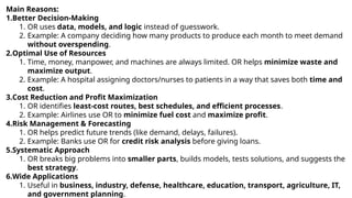
Main Reasons:
1.Better Decision-Making
1.OR uses data, models, and logic instead of guesswork.
2. Example: A company deciding how many products to produce each month to meet demand
without overspending.
2.Optimal Use of Resources
1. Time, money, manpower, and machines are always limited. OR helps minimize waste and
maximize output.
2. Example: A hospital assigning doctors/nurses to patients in a way that saves both time and
cost.
3.Cost Reduction and Profit Maximization
1. OR identifies least-cost routes, best schedules, and efficient processes.
2. Example: Airlines use OR to minimize fuel cost and maximize profit.
4.Risk Management & Forecasting
1. OR helps predict future trends (like demand, delays, failures).
2. Example: Banks use OR for credit risk analysis before giving loans.
5.Systematic Approach
1. OR breaks big problems into smaller parts, builds models, tests solutions, and suggests the
best strategy.
6.Wide Applications
1. Useful in business, industry, defense, healthcare, education, transport, agriculture, IT,
and government planning.
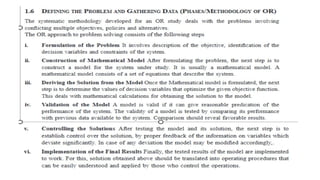
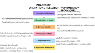
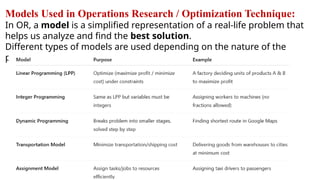
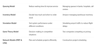
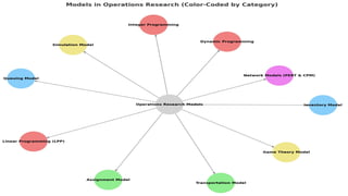
Models Used inOperations Research / Optimization Technique:
In OR, a model is a simplified representation of a real-life problem that
helps us analyze and find the best solution.
Different types of models are used depending on the nature of the
problem.
24.
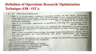
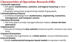
Characteristics of OperationsResearch (OR):
1.Scientific Approach:
1.OR applies mathematics, statistics, and logical reasoning to solve
problems.
2.Example: Using linear programming instead of guesswork.
2.Interdisciplinary Nature:
1.Combines knowledge from mathematics, engineering, economics,
management, and computer science.
3.Decision-Oriented:
1.The main goal is to help managers/decision-makers choose the best
alternative.
4.Optimization:
1.Focuses on finding the best solution (maximum profit, minimum cost, least
time).
5.System Orientation:
1.Considers the organization as a whole system, not just individual parts.
6.Use of Models:
1.Builds mathematical/computer-based models to represent real-life
25.
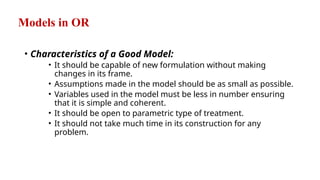
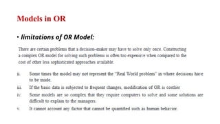
Models in OR
•Characteristics of a Good Model:
• It should be capable of new formulation without making
changes in its frame.
• Assumptions made in the model should be as small as possible.
• Variables used in the model must be less in number ensuring
that it is simple and coherent.
• It should be open to parametric type of treatment.
• It should not take much time in its construction for any
problem.
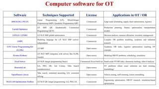
Computer software forOT
Software Techniques Supported License Applications in OT / OR
IBM ILOG CPLEX
Linear Programming (LP), Mixed-Integer
Programming (MIP), Quadratic Programming (QP)
Commercial Large-scale scheduling, supply chain optimization, logistics
Gurobi Optimizer
LP, MIP, QP, Quadratically Constrained
Programming (QCP)
Commercial
Production planning, finance optimization, transportation
models
LINGO / LINDO LP, NLP, MIP, global optimization Commercial Decision analysis, resource allocation, inventory management
AMPL
Modeling language for LP, NLP, MIP (solver-
independent)
Commercial
Complex OR problem modeling, academic and industrial
research
GNU Linear Programming Kit
(GLPK)
LP, MIP Open-source
Academic OR tasks, logistics optimization, teaching OT
concepts
Pyomo (Python)
LP, NLP, MIP (integrates with solvers like GLPK,
Gurobi)
Open-source Modeling OR/OT problems, scheduling, simulation
Excel Solver LP, NLP, integer programming (basic) Commercial (Excel built-in) Small-scale OT/OR tasks, classroom teaching, what-if analysis
HeuristicLab
GA, PSO, DE, Ant Colony, Tabu Search
(metaheuristics)
Open-source
OT problems where exact solutions are hard (routing,
timetabling)
OptaPlanner (Java)
Tabu search, simulated annealing, GA, constraint
solving
Open-source Vehicle routing, staff rostering, course timetabling
MATLAB Optimization Toolbox LP, NLP, QP, integer programming, GA, PSO, SA Commercial
Engineering optimization, OR/OT research, simulation-based
optimization
28.
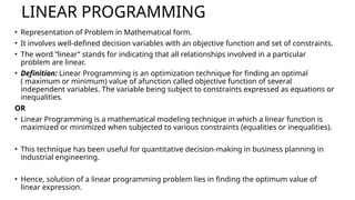
LINEAR PROGRAMMING
• Representationof Problem in Mathematical form.
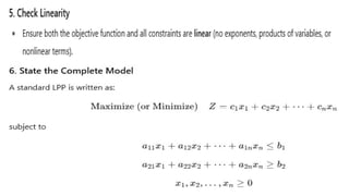
• It involves well-defined decision variables with an objective function and set of constraints.
• The word “linear” stands for indicating that all relationships involved in a particular
problem are linear.
• Definition: Linear Programming is an optimization technique for finding an optimal
( maximum or minimum) value of afunction called objective function of several
independent variables. The variable being subject to constraints expressed as equations or
inequalities.
OR
• Linear Programming is a mathematical modeling technique in which a linear function is
maximized or minimized when subjected to various constraints (equalities or inequalities).
• This technique has been useful for quantitative decision-making in business planning in
industrial engineering.
• Hence, solution of a linear programming problem lies in finding the optimum value of
linear expression.
29.
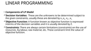
LINEAR PROGRAMMING
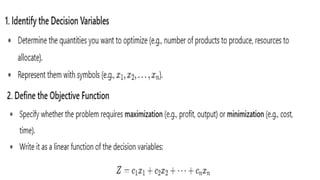
• Componentsof LP Model
Decision Variables: These are the unknowns to be determined subject to
the given constraints, usually these are denoted by x1,x2, x3…xn
Objective Function: A function known as objective function is expressed
interms of the decision variables and it is usually denoted by Z.
Constraints: There are always certain limitations (constraints) on the use of
resources. Eg labour, raw material, etc. These constraint limit the value of
objective function.
30.
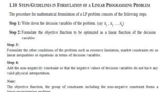
FORMULATION OF LPPROBLEM
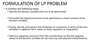
• It involves the following steps:
Identify the decision variables that are to be determined.
Formulate the Objective function to be optimized as a linear function of the
decision variables.
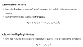
Clearly, identify and express the limitations or constraints in terms of decision
variables in algebraic form either as linear equations or inequalities.
Add non-negativity constraint from the consideration so that the negative
values of the decision variables do not have any valid physical interpretations.
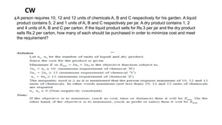
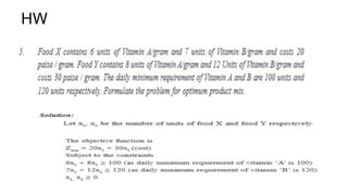
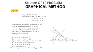
A person requires10, 12 and 12 units of chemicals A, B and C respectively for his garden. A liquid
product contains 5, 2 and 1 units of A, B and C respectively per jar. A dry product contains 1, 2
and 4 units of A, B and C per carton. If the liquid product sells for Rs.3 per jar and the dry product
sells Rs.2 per carton, how many of each should be purchased in order to minimize cost and meet
the requirement?
CW
4
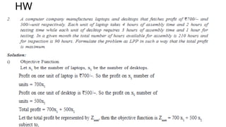
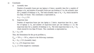
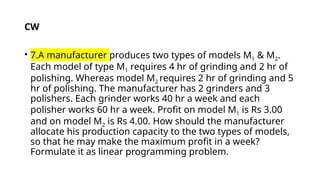
• 7.A manufacturerproduces two types of models M1 & M2.
Each model of type M1 requires 4 hr of grinding and 2 hr of
polishing. Whereas model M2 requires 2 hr of grinding and 5
hr of polishing. The manufacturer has 2 grinders and 3
polishers. Each grinder works 40 hr a week and each
polisher works 60 hr a week. Profit on model M1 is Rs 3.00
and on model M2 is Rs 4.00. How should the manufacturer
allocate his production capacity to the two types of models,
so that he may make the maximum profit in a week?
Formulate it as linear programming problem.
CW
45.
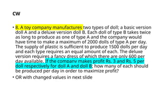
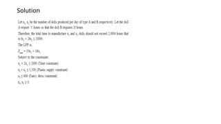
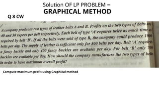
• 8. Atoy company manufactures two types of doll; a basic version
doll A and a deluxe version doll B. Each doll of type B takes twice
as long to produce as one of type A and the company would
have time to make a maximum of 2000 dolls of type A per day.
The supply of plastic is sufficient to produce 1500 dolls per day
and each type requires an equal amount of each. The deluxe
version requires a fancy dress of which there are only 600 per
day available. If the company makes profit Rs. 3 and Rs. 5 per
doll respectively for doll A and doll B; how many of each should
be produced per day in order to maximize profit?
• OR with changed values in next slide
CW
HW
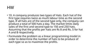
• 10. Acompany produces two types of Hats. Each hat of the
first type requires twice as much labour time as the second
type. If all hats are of the second type only, the company can
produce a total of 500 hats a day. The market limits daily
sales of the first and second type to 150 and 250 hats.
Assuming that the profits per hats are Rs 8 and Rs. 5 for hat
A and B respectively.
• Formulate the problem as a linear programming model in
order to determine the number of hats to be produce of
each type so as to maximize the profits.
50.
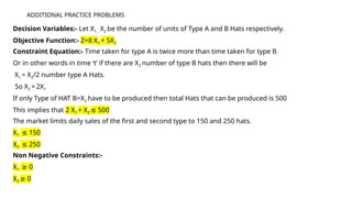
ADDITIONAL PRACTICE PROBLEMS
DecisionVariables:- Let X1 , X2 be the number of units of Type A and B Hats respectively.
Objective Function:- Z=8 X1 + 5X2
Constraint Equation:- Time taken for type A is twice more than time taken for type B
Or in other words in time ‘t’ if there are X2 number of type B hats then there will be
X1 = X2/2 number type A Hats.
So X2 = 2X1
If only Type of HAT B=X2 have to be produced then total Hats that can be produced is 500
This implies that 2 X1 + X2 500
≤
The market limits daily sales of the first and second type to 150 and 250 hats.
X1 150
≤
X2 250
≤
Non Negative Constraints:-
X1 0
≥
X2 0
≥
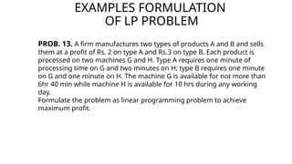
EXAMPLES FORMULATION
OF LPPROBLEM
PROB. 13. A firm manufactures two types of products A and B and sells
them at a profit of Rs. 2 on type A and Rs.3 on type B. Each product is
processed on two machines G and H. Type A requires one minute of
processing time on G and two minutes on H; type B requires one minute
on G and one minute on H. The machine G is available for not more than
6hr 40 min while machine H is available for 10 hrs during any working
day.
Formulate the problem as linear programming problem to achieve
maximum profit.
54.
EXAMPLES FORMULATION
OF LPPROBLEM
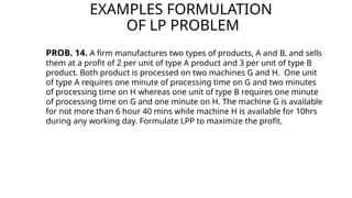
PROB. 14. A firm manufactures two types of products, A and B, and sells
them at a profit of 2 per unit of type A product and 3 per unit of type B
product. Both product is processed on two machines G and H. One unit
of type A requires one minute of processing time on G and two minutes
of processing time on H whereas one unit of type B requires one minute
of processing time on G and one minute on H. The machine G is available
for not more than 6 hour 40 mins while machine H is available for 10hrs
during any working day. Formulate LPP to maximize the profit.
55.
EXAMPLES FORMULATION
OF LPPROBLEM
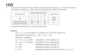
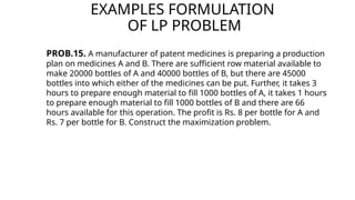
PROB.15. A manufacturer of patent medicines is preparing a production
plan on medicines A and B. There are sufficient row material available to
make 20000 bottles of A and 40000 bottles of B, but there are 45000
bottles into which either of the medicines can be put. Further, it takes 3
hours to prepare enough material to fill 1000 bottles of A, it takes 1 hours
to prepare enough material to fill 1000 bottles of B and there are 66
hours available for this operation. The profit is Rs. 8 per bottle for A and
Rs. 7 per bottle for B. Construct the maximization problem.
56.
EXAMPLES FORMULATION
OF LPPROBLEM
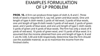
PROB. 16. A firm can produce three types of cloth A, B and C. Three
kinds of wool is required for it, say red, green and blue wools. One unit
length of type A cloth needs 2 yards of red wool, 3 yards of blue wools,
one unit length of type B cloth needs 3 yards of red wool, 2 yards of green
wool, and 2 yards of blue wool, and one unit length of type C cloth needs
5 yards of green and 4 yards of blue wools. The firm has only a stock of 8
yards of red wool, 10 yards of green wool, and 15 yards of blue wool. It is
assumed that the income obtained from one unit length of type A, B and
C are Rs 3.00, 5.00 and 4.00 respectively. Determine how the firm should
use the available material, so as to maximize the income from the
finished cloths
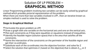
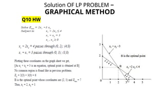
Solution OF LPPROBLEM –
GRAPHICAL METHOD
Linear Programming problem involving two variables can be easily solved by graphical
method which provides pictorial representation of the problem.
When there are more than two variables involved in LPP , then an iterative known as
simplex method is used to solve the problem.
Steps in Graphical Method
Formulate the given problem as LPP.
Draw a graph with one variable on the horizontal axis and one on the vertical axis.
Plot each constraints as if they were equalities or equations instead of inequalities.
Identify the feasible region (solution space) that is the area that satisfies all the
constraints.
Name the intersection of the constraints on the perimeter of the feasible region and
get their co-ordinates.
Substitute each of the co-ordinates into the objective function and solve for Z
Select the solution that optimizes Z ( based on the objective) that is obtain Zmax or Z
Solution OF LPPROBLEM –
GRAPHICAL METHOD
STEPS in Graphical method
STEP1. Write the constraint equation inequalities as equalities.
STEP2. Plot the straight line using the equations obtained in step 1.
STEP3. Find the coordinates of corner points of feasible region.
If the inequality constraint corresponds to then the region below the line lying on first
≤
quadrant is shaded.
If the inequality constraint corresponds to then the region above the line lying on first
≥
quadrant is shaded. The points lying in the common region will satisfy all the constraints and
the common region is called Feasible region.
Step4. Locate the corner points of feasible region and compute the value of Z for these
coordinates.
Step5. Identify the maximum or minimum, as per requirement, objective function value from
the values calculated in step 4.
61.
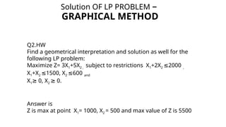
Solution OF LPPROBLEM –
GRAPHICAL METHOD
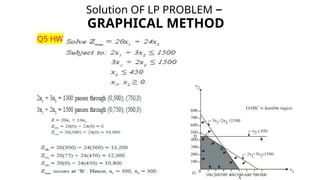
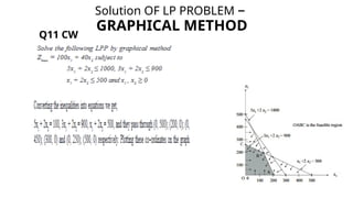
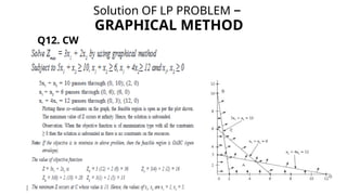
Q2.HW
Find a geometrical interpretation and solution as well for the
following LP problem:
Maximize Z= 3X1+5X2 , subject to restrictions X1+2X2 2000
≤ ,
X1+X2 1500, X
≤ 2 600
≤ and
X1 0, X
≥ 2 0.
≥
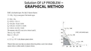
Answer is
Z is max at point X1= 1000, X2 = 500 and max value of Z is 5500
Solution OF LPPROBLEM –
GRAPHICAL METHOD
SPECIAL CASES IN GRAPHICAL METHOD
76.
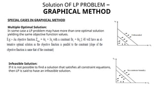
Solution OF LPPROBLEM –
GRAPHICAL METHOD
SPECIAL CASES IN GRAPHICAL METHOD
Multiple Optimal Solution:
In some case a LP problem may have more than one optimal solution
yielding the same objective function values.
Infeasible Solution:
If it is not possible to find a solution that satisfies all constraint equations,
then LP is said to have an infeasible solution.
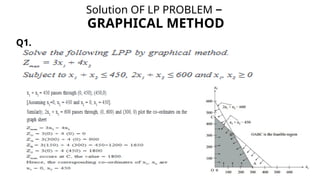
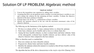
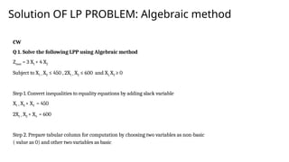
Solution OF LPPROBLEM: Algebraic method
CW
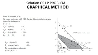
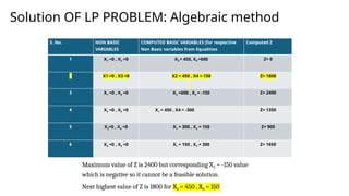
Q 1. Solve the following LPP using Algebraic method
Zmax = 3 X1 + 4 X2
Subject to X1 + X2 ≤ 450 , 2X1 + X2 ≤ 600 and X1, X2 ≥ 0
Step 1. Convert inequalities to equality equations by adding slack variable
X1 + X2 + X3 = 450
2X1 + X2 + X4 = 600
Step 2. Prepare tabular column for computation by choosing two variables as non-basic
( value as 0) and other two variables as basic
82.
Solution OF LPPROBLEM: Algebraic method
S. No. NON BASIC
VARIABLES
COMPUTED BASIC VARIABLES [for respective
Non Basic variables from Equalities
Computed Z
1 X1 =0 , X2 =0 X3 = 450, X4 =600 Z= 0
2 X1 =0 , X3 =0 X2 = 450 , X4 = 150 Z= 1800
3 X1 =0 , X4 =0 X2 =600 , X3 = -150 Z= 2400
4 X2 =0 , X3 =0 X1 = 450 , X4 = -300 Z= 1350
5 X2=0 , X4 =0 X1 = 300 , X3 = 150 Z= 900
6 X3 =0 , X4 =0 X1 = 150 , X2 = 300 Z= 1650
Maximum value of Z is 2400 but corresponding X3 = -150 value
which is negative so it cannot be a feasible solution.
Next highest value of Z is 1800 for X2 = 450 , X4 = 150
83.
Solution OF LPPROBLEM: Algebraic method
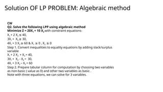
CW
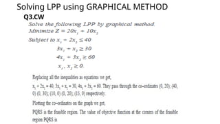
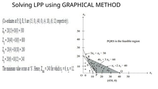
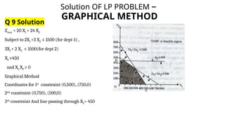
Q2. Solve the following LPP using algebraic method
Minimize Z = 20X1 + 10 X2 with constraint equations-
X1 + 2 X2 40,
≤
3X1 + X2 30,
≥
4X1 + 3 X2 60 & X
≥ 1 0 , X
≥ 2 0
≥
Step 1. Convert inequalities to equality equations by adding slack/surplus
variable
X1 + 2 X2 + X3 = 40,
3X1 + X2 - X4 = 30,
4X1 + 3 X2 – X5 = 60
Step 2. Prepare tabular column for computation by choosing two variables
as non-basic ( value as 0) and other two variables as basic .
Note with three equations, we can solve for 3 variables.
84.
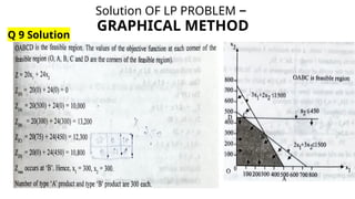
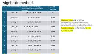
Algebraic method
S. No.NON BASIC VARIABLES COMPUTED BASIC VARIABLES [for
respective Non Basic variables from
Equalities
Computed Z
Z = 20X1 + 10 X2
1 X1 =0 , X2 =0 X3 = 40, X4 = - 30, X5 = - 60 Z= 0
2 X1 =0 , X3 =0 X2 = 20, X4 = -10, X5=0 Z= 200
3 X1 =0 , X4 =0 X2 =30 , X3 = -20, X5=30 Z= 300
4 X2 =0 , X3 =0 X1 = 40 , X4 = 90, X5=100 Z= 800
5 X2=0 , X4 =0 X1 = 10 , X3 = 30, X5= - 20 Z= 200
6 X3 =0 , X4 =0 X1 = 4 , X2 = 18, X5= 10 Z= 260
7 X1 =0 , X5 =0 X2 = 20 , X3 = 0, X4= -10 Z= 400
8 X2 =0 , X5 =0 X1 = 15 , X3 = 25, X4= 15 Z= 300
9 X3 =0 , X5 =0 X1 = 0 , X2 = 20, X4= -10 Z= 200
Minimum value of Z is 200 but
corresponding negative values of the
variables so it cannot be a feasible solution.
Next lowest value of Z is 240 for X1 = 6 ,
X2 = 12, X3 =10