SlideShare a Scribd company logo
1 of 90
Download to read offline
Model-driven decision support for
monitoring network design based on
analysis of data and model uncertainties:
methods and applications
Velimir V Vesselinov1, Dylan Harp1, Danny Katzman2
1 Computational Earth Sciences, Earth and Environmental Sciences,
2 Environmental Programs,
Los Alamos National Laboratory (LANL), Los Alamos, NM
AGU Fall Meeting 2012
H32F. Uncertainty Quantification and Parameter Estimation:
Impacts on Risk and Decision Making
December 5, 2012
San Francisco, CA
LA-UR-12-26681
Outline
 Model-driven (model-based) decision support
 Probabilistic vs Non-Probabilistic Decision Methods
 Information Gap (info-gap) Decision Theory
 Information Gap (info-gap) Applications:
o Monitoring Network Design
o Contaminant Remediation through Source Control
 Decision Support for Chromium contamination site @ LANL
 MADS: Model Analyses & Decision Support
Open source C/C++ computational framework
Publications, examples & tutorials @
http://mads.lanl.gov
 ASCEM: Advanced Subsurface Computing for
Environmental Management; Multi-national lab code
development project http://ascemdoe.org (U.S. DOE)
Model-driven (model-based) decision support
 provides decision makers (DM) with model analysis of decision
scenarios taking into account site data and knowledge including existing
uncertainties (uncertainties in conceptualization, model parameters,
and model predictions)
 Model analysis: evaluation, ranking and optimization of alternative
decision scenarios
 Decision metric(s): e.g. contaminant concentration at a monitoring well
(environmental risk at a point of compliance)
 Decision goal(s): e.g. no exceedance of MCL at a compliance point
and/or increase chance of detecting exceedance of MCL at a monitoring
well
 Decision scenarios: combinations of predefined activities to achieve the
decision goal(s)
Model-driven decision support (cont.)
 Activities:
o data acquisition campaigns
o field/lab experiments
o monitoring
o remediation
 Activities are analyzed in terms of their impact on decision making
process (decision uncertainties)
 Decision uncertainties: uncertainties associated with selection of
optimal decision scenarios, or performance of specific decision scenarios
 The Game: Decision maker (DM) vs Nature
Important:
 activities are selected only to reduce decision uncertainties
 activities are not selected to reduce model or parameter uncertainties
per se (unconstrained problem).
Non-Probabilistic Decision Methods
 Lack of knowledge or information precludes decision analyses requiring
unbiased probabilistic distributions or frequency of occurrence (e.g. Bayesian
approaches)
 Severe uncertainties (black swans, dragon kings) can have important impact in
the decision analyses
 Non-probabilistic decision methods can be applied to effectively incorporate
lack of knowledge and severe uncertainties in decision making process
o Minimax (Maximin) Theory (Wald, 1951)
o Information Gap Decision Theory (Ben-Haim, 2006)
 Non-Probabilistic and Probabilistic methods can be coupled (e.g. unknown
probability distribution parameters can be a subject of non-probabilistic
analysis, e.g. info-gap)
Information Gap Decision Theory
 Nominal (“best”) model prediction intended for decision making
(based on nominal / “best estimates” model parameter set)
 Decision metric(s) / performance goal(s)
 Decision scenarios: vector of alternative decisions d to compare
 Info-Gap Uncertainty Model (info-gap uncertainty metric = α)
o energy bound (functional uncertainties: objective function, forcing
functions, etc.)
o envelope bound (domain uncertainties: model parameters, calibration
targets, etc.)
o nested sets of uncertain model entities ranked by the largest information
gap α that can be included in the set
o uncertain model entities: parameters, calibrations, functions, etc. with info-
gap uncertainties
o e.g. U(α,T) = { T: abs(T-T’) < α } where T’ are the nominal values for
uncertain model entities
 Model predictions C(d) constrained by U(α,T)
Ben-Haim (2006). Info-gap decision theory: decisions under severe uncertainty. Academic Press.
Information Gap Decision Theory
 Decision uncertainty is bounded by robustness and opportuness functions
 Robustness function (immunity to failure of alternate decisions d)
o defines the maximum horizon of uncertainty
o R(d) = max{ α: performance goal is satisfied }
e.g. R(d) = max{ α: ( max C(d) ) < MCL }
 Opportuness function (immunity to windfall of alternate decisions d)
o defines the minimum horizon of uncertainty
o O(d) = min{ α: performance goal is satisfied }
e.g. O(d) = min{ α: ( min C(d) ) < MCL }
 Analyses based on Decision Robustness and/or Decision Opportuness:
o Model selection
o Remedy selection
o Performance assessment
o …
Ben-Haim (2006). Info-gap decision theory: decisions under severe uncertainty. Academic Press.
Info-Gap Analysis: Model parameters
Nominal
parameter set
Parameter 1
Parameter2
Contaminant concentration [ppb]
Info-gapuncertaintymetricα
MCL
Nominal
prediction
0.1 1 10 100
1
2
3
4
Bayesian Analysis: Model parameters
“Best”
parameter set
Parameter 1
Parameter2
Contaminant concentration [ppb]
Probability
MCL
“Best”
prediction
0.1 1 10 100
Bayesian Analysis: Model parameters
“Best”
parameter set
Parameter 1
Parameter2
Contaminant concentration [ppb]
Probability
MCL
“Best”
prediction
0.1 1 10 100
Bayesian Analysis: Model parameters
“Best”
parameter set
Parameter 1
Parameter2
Contaminant concentration [ppb]
Probability
MCL
“Best”
prediction
0.1 1 10 100
… the challenge is in
tail characterization
Info-Gap Analysis: Model parameters (envelope bounds)
Parameter 1
Parameter2
Contaminant concentration [ppb]
MCL
Nominal
prediction
0.1 1 10 100
Nominal
parameter set
1
2
3
4
Info-gapuncertaintymetricα
Info-Gap Analysis: Model parameters (envelope bounds)
Nested
parameter
sets
Parameter 1
Parameter2
Contaminant concentration [ppb]
MCL
Nominal
prediction
0.1 1 10 100
1
2
3
4
Info-gapuncertaintymetricα
α1 α2
α3
α4
info-gap uncertainty metric = α
α1 < α2 < α3 < α4
Info-Gap Analysis: Model parameters (envelope bounds)
Nested
parameter
sets
Parameter 1
Parameter2
Contaminant concentration [ppb]
MCL
Nominal
prediction
0.1 1 10 100
1
2
3
4
Info-gapuncertaintymetricα
α1 α2
α3
α4
info-gap uncertainty metric = α
α1 < α2 < α3 < α4
min{α1: C}
min{α2: C}
min{α3: C}
max{α1: C}
max{α2: C}
max{α3: C}
Info-Gap Analysis: Model parameters (envelope bounds)
Nested
parameter
sets
Parameter 1
Parameter2
Contaminant concentration [ppb]
MCL
Nominal
prediction
0.1 1 10 100
1
2
3
4
Info-gapuncertaintymetricα
α1 α2
α3
α4
info-gap uncertainty metric = α
α1 < α2 < α3 < α4
Decision
uncertainty
min{α1: C}
min{α2: C}
min{α3: C}
max{α1: C}
max{α2: C}
max{α3: C}
Info-Gap Analysis: Calibration Targets (envelope bounds)
Calibration target 1
Calibrationtarget2
Contaminant concentration [ppb]
MCL
Nominal
prediction
0.1 1 10 100
Nominal
calibration
target
1
2
3
4
Info-gapuncertaintymetricα
Parameter 1
Parameter2
Nominal
parameter set
Inversion
Info-Gap Analysis: Calibration Targets (envelope bounds)
Nested
calibration
sets
Calibration target 1
Calibrationtarget2
Contaminant concentration [ppb]
MCL
Nominal
prediction
0.1 1 10 100
1
2
3
4
Info-gapuncertaintymetricα
Parameter 1
Parameter2
Nominal
parameter set
Inversion
Info-Gap Analysis: Calibration Targets (envelope bounds)
Nested
calibration
sets
Calibration target 1
Calibrationtarget2
Contaminant concentration [ppb]
MCL
Nominal
prediction
0.1 1 10 100
1
2
3
4
Info-gapuncertaintymetricαParameter
sets
Parameter 1
Parameter2
Inversion
Info-Gap Analysis: Calibration Targets (envelope bounds)
Nested
calibration
sets
Calibration target 1
Calibrationtarget2
Contaminant concentration [ppb]
MCL
Nominal
prediction
0.1 1 10 100
1
2
3
4
Info-gapuncertaintymetricαParameter
sets
Parameter 1
Parameter2
Inversion
min{α1: C}
min{α2: C}
min{α3: C}
max{α1: C}
max{α2: C}
max{α3: C}
Info-Gap Analysis: Decision selection based on robustness
Contaminant concentration [ppb]
MCL
Nominal
prediction
0.1 1 10 100
1
2
3
4
Info-gapuncertaintymetricα
Info-Gap Analysis: Decision selection based on robustness
Contaminant concentration [ppb]
MCL
Nominal
prediction
0.1 1 10 100
1
2
3
4
Info-gapuncertaintymetricα
“Strong”
robustness
Info-Gap Analysis: Decision selection based on robustness
Contaminant concentration [ppb]
MCL
Nominal
prediction
0.1 1 10 100
1
2
3
4
Info-gapuncertaintymetricα
“Strong”
robustness
“Weak”
robustness
Info-Gap Analysis: Decision selection based on robustness
Contaminant concentration [ppb]
MCL
Nominal
prediction
0.1 1 10 100
1
2
3
4
Info-gapuncertaintymetricα
“Strong”
robustness
“Weak”
robustness
Info-Gap Analysis: Decision selection based on robustness
Contaminant concentration [ppb]
MCL
Nominal
prediction
0.1 1 10 100
1
2
3
4
Info-gapuncertaintymetricα
“Strong”
robustness
“Weak”
robustness
Info-Gap Analysis: Decision selection based on robustness
Contaminant concentration [ppb]
MCL
Nominal
prediction
0.1 1 10 100
1
2
3
4
Info-gapuncertaintymetricα
“Strong”
robustness
“Weak”
robustness
Info-gapuncertaintymetricαInfo-Gap Analysis: Model selection based on robustness
Contaminant concentration [ppb]
MCL
Nominal
prediction
0.1 1 10 100
1
2
3
4
“Strong”
robustness
“Weak”
robustness
Info-gapuncertaintymetricαInfo-Gap Analysis: Model selection based on robustness
Contaminant concentration [ppb]
MCL
Nominal
prediction
0.1 1 10 100
1
2
3
4
“Strong”
robustness
“Weak”
robustness
Info-gapuncertaintymetricαInfo-Gap Analysis: Model selection based on robustness
Contaminant concentration [ppb]
MCL
Nominal
prediction
0.1 1 10 100
1
2
3
4
“Strong”
robustness
“Weak”
robustness
Model complexity (representativeness)
Model 1 < Model 2 < Model 3
Info-gapuncertaintymetricαInfo-Gap Analysis: Model selection based on robustness
Contaminant concentration [ppb]
MCL
Nominal
prediction
0.1 1 10 100
1
2
3
4
“Strong”
robustness
“Weak”
robustness
Model complexity (representativeness)
Model 1 < Model 2 < Model 3
Info-Gap Analysis: Decision selection based on opportuness
Contaminant concentration [ppb]
MCL
Nominal
prediction
0.1 1 10 100
1
2
3
4
Info-gapuncertaintymetricα
Info-Gap Analysis: Decision selection based on opportuness
Contaminant concentration [ppb]
MCL
Nominal
prediction
0.1 1 10 100
1
2
3
4
Info-gapuncertaintymetricα
“Weak”
opportuness
Info-Gap Analysis: Decision selection based on opportuness
Contaminant concentration [ppb]
MCL
Nominal
prediction
0.1 1 10 100
1
2
3
4
Info-gapuncertaintymetricα
“Weak”
opportuness
“Strong”
opportuness
Info-Gap Analysis: Decision selection based on opportuness
Contaminant concentration [ppb]
MCL
Nominal
prediction
0.1 1 10 100
1
2
3
4
Info-gapuncertaintymetricα
“Weak”
opportuness
“Strong”
opportuness
Info-gapuncertaintymetricαInfo-Gap Analysis: Decision uncertainty
Contaminant concentration [ppb]
MCL
Nominal
prediction
0.1 1 10 100
1
2
3
4
… duality of decision uncertainty
propitious pernicious
Decision uncertainty
Info-gapuncertaintymetricαInfo-Gap Analysis: Decision uncertainty
Contaminant concentration [ppb]
MCL
Nominal
prediction
0.1 1 10 100
1
2
3
4
… not preferred decision bounds
Info-gapuncertaintymetricαInfo-Gap Analysis: Decision uncertainty
Contaminant concentration [ppb]
MCL
Nominal
prediction
0.1 1 10 100
1
2
3
4
… preferred decision bounds
Info-Gap Application: Case 1
Optimization of monitoring network
Info-Gap Analysis: Network Design
100
40
0.5
0.5
0.5
0.5
0.5
0.5
0.5
0.5
 Two monitoring wells in an aquifer with contaminant
concentrations above MCL (5 ppm)
 Background concentration = 0.5 ppm
MCL = 5 Background = 0.5
100
40
0.5
0.5
0.5
0.5
0.5
0.5
0.5
0.5
 4 new proposed monitoring well locations
 Which well has the highest immunity to fail in
detection contaminants above MCL?
Info-Gap Analysis: Network Design
MCL = 5 Background = 0.5
Info-Gap Analysis: Network Design
100
40
0.5
0.5
0.5
0.5
0.5
0.5
0.5
0.5
 Where is the contaminant source?
MCL = 5 Background = 0.5
Info-Gap Analysis: Network Design
100
40
0.5
0.5
0.5
0.5
0.5
0.5
0.5
0.5
 Where is the contaminant source?
MCL = 5 Background = 0.5
Info-Gap Analysis: Network Design
100
40
0.5
0.5
0.5
0.5
0.5
0.5
0.5
0.5
 Where is the contaminant source?
MCL = 5 Background = 0.5
Info-Gap Analysis: Network Design
100
40
0.5
0.5
0.5
0.5
0.5
0.5
0.5
0.5
 Where is the contaminant source?
MCL = 5 Background = 0.5
100
40
0.5
0.5
0.5
0.5
0.5
0.5
0.5
0.5
170
0.5
0.5
0.5
c > 5 (MCL)
Info-Gap Analysis: Network Design
MCL = 5 Background = 0.5
100
40
0.5
0.5
0.5
0.5
0.5
0.5
0.5
0.5
170
0.5
0.5
0.5
c > 5 (MCL)
Info-Gap Analysis: Network Design
MCL = 5 Background = 0.5
100
40
0.5
0.5
0.5
0.5
0.5
0.5
0.5
0.5
c > 5 (MCL)
Info-Gap Analysis: Network Design
MCL = 5 Background = 0.5
100
40
0.5
0.5
0.5
0.5
0.5
0.5
0.5
0.5
c > 5 (MCL)
Info-Gap Analysis: Network Design
MCL = 5 Background = 0.5
100
40
0.5
0.5
0.5
0.5
0.5
0.5
0.5
0.5
c > 5 (MCL)
Info-Gap Analysis: Network Design
MCL = 5 Background = 0.5
100
40
0.5
0.5
0.5
0.5
0.5
0.5
0.5
0.5
c > 5 (MCL)
Info-Gap Analysis: Network Design
MCL = 5 Background = 0.5
100
40
0.5
0.5
0.5
0.5
0.5
0.5
0.5
0.5
c > 5 (MCL)
Info-Gap Analysis: Network Design
MCL = 5 Background = 0.5
Info-Gap Analysis: Network Design
 Analytical contaminant flow model:
o 3D steady-state uniform groundwater flow in unbounded aquifer
o 3D contaminant source at the top of the aquifer
o 3D contaminant migration (advection, dispersion)
 Deterministic model parameters
o contaminant flux at the contaminant source
o contaminant arrival time
o groundwater velocity
o source thickness (zS = 1 m)
Info-Gap Analysis: Network Design
 Unknown model parameters (8)
o source coordinates (x, y)
o source size (xS, yS)
o flow direction
o aquifer dispersivities (longitudinal, horizontal/vertical transverse)
 Uncertain observations (calibration targets) (10):
o concentrations at the monitoring wells
 Unknown model parameters estimated using inversion
 Impact of uncertainty in calibration targets on model parameters is
estimated using info-gap analyses
 Robustness and opportuness functions associated with predicted
contaminant concentrations at the proposed new well locations are
applied for decision analyses
 Decision question: which of the new proposed well location has the
highest immunity of failure/windfall to detect concentrations above
MCL (c > 5 ppm)
i.e. which well provides the most robust/opportune decision to
improve the monitoring network
Info-Gap Analysis: Network Design
 Calibration targets are highly uncertain (PDF’s cannot be defined) due to:
o measurement errors
o uncertain background concentrations
o uncertain local hydrogeological and geochemical conditions
0.5
0.01
0.1
1
10
0.1 1 10
100
40
0.5
0.5
0.5
0.5
0.5
0.5
0.5
Info-Gap Analysis:
Network Design
MCL = 5 Background = 0.5
MCL0.5
Wb Wc Wa
Info-gapuncertaintymetricα Predicted concentrations vs Info-gap uncertainty
Nominal =
opportuness
0.01
0.1
1
10
0.1 1 10 100 1000
100
40
0.5
0.5
0.5
0.5
0.5
0.5
0.5
Info-Gap Analysis:
Network Design
MCL = 5 Background = 0.5
MCL0.5
Wb Wc Wa
Info-gapuncertaintymetricα Predicted concentrations vs Info-gap uncertainty
Wd opportuness Wd robustness
Wd
nominal
Info-Gap Application: Case 2
Remediation of contamination in a aquifer through contaminant source control
Harp & Vesselinov (2011). Contaminant remediation decision analysis using information gap theory. SERRA.
Info-Gap Analysis: Remediation of contaminant source
Compliance
point
Aquifer
Vadose
zone
transport
Ground surfaceSpill
Surface flow
Precipitation
Snow melt ?
?
?
?
Distance x’
C(x’,t)I(t)
Harp & Vesselinov (2011). Contaminant remediation decision analysis using information gap theory. SERRA.
Simple contaminant remediation problem:
 how much contaminant mass needs to be removed to satisfy compliance
requirement C(x’,t) < MCL
 lack of probabilistic (frequency of occurrence) information about the contaminant
mass flux to aquifer I(t)
0
200
400
600
800
1000
0 10 20 30
Info-Gap Analysis: Remediation of contaminant source
Time since contaminant release [a]
Contaminantflux[kg/m/a]
I(t)=1000 exp(-0.05t)
Contaminant mass flux to the aquifer I(t)
0
200
400
600
800
1000
0 10 20 30
Info-Gap Analysis: Remediation of contaminant source
Time since contaminant release [a]
Contaminantflux[kg/m/a]
Contaminant mass flux uncertainty bounds
info-gap uncertainty metric = α
α1
α2
α3 α4
0
200
400
600
800
1000
0 10 20 30
Info-Gap Analysis: Remediation of contaminant source
Time since contaminant release [a]
Contaminantflux[kg/m/a]
Contaminant mass flux plausible scenarios
(energy bound)
Info-Gap Analysis: Remediation of contaminant source
Time since contaminant release [a]
Contaminantflux[kg/m/a]
0
200
400
600
800
1000
0 10 20 30
0.0
0.1
0.5
0.9
Fraction of
contaminant mass
removed q
I(t)=1000 (1-q) exp(-0.05t)
Time since release [a]
Infinite robustness is achieved
when all the contaminant mass
is removed
Decisionrobustness
Fraction of
mass removed
Info-Gap Analysis: Remediation of contaminant source
Decision robustness defines how much contaminant mass should be removed and still be
immune to failure considering lack of information about the contaminant mass flux
Fraction of the contaminant mass removed
All mass removed
No mass removed
Infinite robustness is
achieved when all the
mass is removed
Decision robustness increases
with the fraction of mass
removed
Decisionrobustness
Time since
contaminant
release
Decision robustness varies (increases/decreases) with the time
since remediation; αmin (dashed line) defines the minimum
robustness for a given fraction of the mass removed
Info-Gap Analysis: Remediation of contaminant source
Chromium plume in the regional aquifer at LANL
GOALS:
 provide model-based decision support related to chromium
transport in the vadose zone and regional aquifer at LANL
 apply advanced computationally efficient methods for:
o parameter estimation (PE)
o model calibration
o model-based uncertainty quantification (UQ)
o risk analysis (RA), and
o decision support (DS)
 utilize high-performance computing due to high computational
demands for model simulations and model analyses
Chromium plume in the regional aquifer at LANL
Vadose zone monitoring wells
Chromium plume in the regional aquifer at LANL
Regional monitoring wells
Vadose zone monitoring wells
Chromium plume in the regional aquifer at LANL
Supply wells
Regional monitoring wells
Vadose zone monitoring wells
Chromium plume in the regional aquifer at LANL
Supply wells
Regional monitoring wells
Vadose zone monitoring wells
Cr concentrations (~2012) [ppb]
MCL = 5 ppb
Background 5-8 ppb
N
Water
supply well
PM-3
Vadosezone(~300m)
N
Water
supply well
PM-3
Vadosezone(~300m)
N
Water
supply well
PM-3
Vadosezone(~300m)
N
Water
supply well
PM-3
Vadosezone(~300m)
Cr6+
~54,000 kg
N
Water
supply well
PM-3
Vadosezone(~300m)
Cr6+
~54,000 kg
N
Water
supply well
PM-3
Vadosezone(~300m)
Cr6+
~54,000 kg
N
Water
supply well
PM-3
Vadosezone(~300m)
Cr6+
~54,000 kg
N
Water
supply well
PM-3
Vadosezone(~300m)
Cr6+
~54,000 kg
Cr6+ ~5,600 kg
Cr3+ ~17,000 kg
N
Water
supply well
PM-3
Vadosezone(~300m)
Cr6+
~54,000 kg
Cr6+ ~5,600 kg
Cr3+ ~17,000 kg
Cr6+ ~230 kg
Cr3+ ~2 kg
N
Water
supply well
PM-3
Vadosezone(~300m)
Cr6+
~54,000 kg
Cr6+ ~5,600 kg
Cr3+ ~17,000 kg
Cr6+ ~230 kg
Cr3+ ~2 kg
Cr6+ ~3,000 kg
Cr3+ ~9,000 kg
N
Cr6+
> 50 ppb
Cr6+
>400 ppb
Water
supply well
PM-3
Vadosezone(~300m)
Cr6+
> 100 ppb
Cr6+
~54,000 kg
Cr6+ ~5,600 kg
Cr3+ ~17,000 kg
Cr6+ ~230 kg
Cr3+ ~2 kg
Cr6+ ~3,000 kg
Cr3+ ~9,000 kg
2009 model estimate of the plausible contaminant
concentrations [ppb] along the regional aquifer water table
 Wells R-62, R-61 and R-50 were not drilled yet
 Locations of wells R-62, R-61 and R-50 were optimized based on model analyses
 Observed concentrations at R-62, R-61 and R-50 confirmed model predictions
 R-43 concentration were at background when the analyses were performed
 Since 2010, R-43 concentrations are increasing and approaching the model
predicted concentration
MCL = 50 ppb
2009 model estimate of the plausible contaminant
concentrations [ppb] along the regional aquifer water table
 Wells R-62, R-61 and R-50 were not drilled yet
 Locations of wells R-62, R-61 and R-50 were optimized based on model analyses
 Observed concentrations at R-62, R-61 and R-50 confirmed model predictions
 R-43 concentration were at background when the analyses were performed
 Since 2010, R-43 concentrations are increasing and approaching the model
predicted concentration
100
~30-200
MCL = 50 ppb
18
2009 model estimate of the plausible contaminant
concentrations [ppb] along the regional aquifer water table
 Wells R-62, R-61 and R-50 were not drilled yet
 Locations of wells R-62, R-61 and R-50 were optimized based on model analyses
 Observed concentrations at R-62, R-61 and R-50 confirmed model predictions
 R-43 concentration were at background when the analyses were performed
 Since 2010, R-43 concentrations are increasing and approaching the model
predicted concentration
100
~30-200
MCL = 50 ppb
~40
18
MADS is applied to perform all the presented info-gap decision analyses …
 an open-source high-performance computational framework for analyses and
decision support based on complex process models
 advanced adaptive computational techniques:
o sensitivity analysis (local / global);
o uncertainty quantification (local / global);
o optimization / calibration / parameter estimation (local / global);
o model ranking & selection
o decision support (GLUE, info-gap)
 novel algorithms
o Agent-Based Adaptive Global Uncertainty and Sensitivity (ABAGUS)
Harp & Vesselinov (2012) An agent-based approach to global uncertainty and sensitivity analysis. Computers & Geosciences.
o Adaptive hybrid (local/global) optimization strategy (Squads)
Vesselinov & Harp (2012) Adaptive hybrid optimization strategy for calibration and parameter estimation of physical process
models. Computers & Geosciences.
 internal coupling with analytical contaminant transport solvers and test problems
 external coupling with existing process simulators (ModFlow, TOUGH, FEHM,
eSTOMP, Amanzi, …)
 Source code, examples, performance comparisons, and tutorials @
http://mads.lanl.gov
Advanced Subsurface Computing for Environmental Management
 an open-source interactive decision support system
(Akuna/Agni) coupled a process simulator (Amanzi)
 high-performance computing (HPC)
 data- and model-driven decision support to provide
standardized, consistent, site-specific and scientifically
defensible decision analyses across DOE-EM complex
 Challenge:
o develop tools to make better use of complex information
and capabilities to explore problems in greater detail
o address the most challenging performance assessment and
waste-disposal problems
 Impact:
o provide technical underpinnings for current U.S. DOE-EM
risk and performance assessments
o inform strategic data collection for model improvement and
decision support
o support scientifically defensible and standardized
assessments and remedy selections
Regulatory
Public Interface
Reviews
Decision Making
Scientific
Model Setup and Execution
Model Analyses
Decision Support
Programmatic
Project Management
Oversight
Decision Making
http://ascemdoe.org
AMANZI
AKUNA
AGNI
Modules
Akuna (“no worries”): Graphic User Interface
(Karen Schuchardt, PNNL)
• Open Source Eclipse/Java based
• Incorporates data management, visualization, and model
development tools
Agni (“fire”): Simulation controller and Toolset driver
(George Pau, LBNL, Velimir Vesselinov, LANL)
• Open Source C++ object oriented
• Provides coupling between Akuna and Amanzi
• Performs various model-based analyses (SA, UQ, PE, DS, … )
Amanzi (“water”): HPC Flow and Transport Simulator
(David Moulton, LANL)
• Open Source C++ object oriented
• Saturated / unsaturated groundwater flow, …
• Structured / unstructured / adaptive gridding
• …
http://ascemdoe.org
Model-Analysis Toolsets in Agni
o Sensitivity Analysis (SA) (Stefan Finsterle, Elizabeth Keating)
o Parameter Estimation (PE) (Stefan Finsterle, LBNL)
o Uncertainty Quantification (UQ) (Elizabeth Keating, LANL)
o Risk Assessment (RA) (Wilson McGinn, ORNL)
o Decision Support (DS) (Velimir Vesselinov, LANL)
http://ascemdoe.org
Conclusions and recommendations:
 Both Non-Probabilistic and Probabilistic uncertainties often exist in a decision
problem
 Non-Probabilistic and Probabilistic methods should be applied to their
appropriate uncertainties in the decision analyses
 In the case of probabilistic methods, definition of prior probability distributions
for model parameters or calibration targets with unknown/uncertain distribution
can produce biased predictions and decision analyses
 In the case of non-probabilistic methods, lack of knowledge and severe
uncertainties can be captured
 Non-probabilistic methodologies have been successfully applied for a series of
synthetic and real-world problems, though less often in hydrology
o Remediation of unknown contaminant source
Harp & Vesselinov (2011). Contaminant remediation decision analysis using information gap theory. SERRA
 MADS provides a computationally efficient framework for decision analyses using
non-probabilistic and probabilistic methods ( http://mads.lanl.gov )
 ASCEM tools are currently actively developed and will become available for
testing and benchmarking in 2013 ( http://ascemdoe.org )
Model-driven decision support for monitoring network design

More Related Content

Similar to Model-driven decision support for monitoring network design

Data and Model-Driven Decision Support for Environmental Management of a Chro...
Data and Model-Driven Decision Support for Environmental Management of a Chro...Data and Model-Driven Decision Support for Environmental Management of a Chro...
Data and Model-Driven Decision Support for Environmental Management of a Chro...Velimir (monty) Vesselinov
 
Intro to Model Selection
Intro to Model SelectionIntro to Model Selection
Intro to Model Selectionchenhm
 
P.M.Pardalos - On Big Data Application
P.M.Pardalos - On Big Data ApplicationP.M.Pardalos - On Big Data Application
P.M.Pardalos - On Big Data ApplicationEkaterina Morozova
 
Raskob Iscram 2009
Raskob Iscram 2009Raskob Iscram 2009
Raskob Iscram 2009guestee5a52
 
FUNCTION OF RIVAL SIMILARITY IN A COGNITIVE DATA ANALYSIS

FUNCTION OF RIVAL SIMILARITY IN A COGNITIVE DATA ANALYSIS

FUNCTION OF RIVAL SIMILARITY IN A COGNITIVE DATA ANALYSIS
Maxim Kazantsev
 
Detecting Discontinuties in Large Scale Systems
Detecting  Discontinuties in Large Scale SystemsDetecting  Discontinuties in Large Scale Systems
Detecting Discontinuties in Large Scale Systemsharoonmalik786
 
2. visualization in data mining
2. visualization in data mining2. visualization in data mining
2. visualization in data miningAzad public school
 
algorithmic-decisions, fairness, machine learning, provenance, transparency
algorithmic-decisions, fairness, machine learning, provenance, transparencyalgorithmic-decisions, fairness, machine learning, provenance, transparency
algorithmic-decisions, fairness, machine learning, provenance, transparencyPaolo Missier
 
Data Mining In Market Research
Data Mining In Market ResearchData Mining In Market Research
Data Mining In Market Researchjim
 
Data Mining in Market Research
Data Mining in Market ResearchData Mining in Market Research
Data Mining in Market Researchbutest
 
Data Mining In Market Research
Data Mining In Market ResearchData Mining In Market Research
Data Mining In Market Researchkevinlan
 
Modeling strategies for definitive screening designs using jmp and r
Modeling strategies for definitive  screening designs using jmp and rModeling strategies for definitive  screening designs using jmp and r
Modeling strategies for definitive screening designs using jmp and rPhilip Ramsey
 
Datascience101presentation4
Datascience101presentation4Datascience101presentation4
Datascience101presentation4Salford Systems
 
DMDW Lesson 05 + 06 + 07 - Data Mining Applied
DMDW Lesson 05 + 06 + 07 - Data Mining AppliedDMDW Lesson 05 + 06 + 07 - Data Mining Applied
DMDW Lesson 05 + 06 + 07 - Data Mining AppliedJohannes Hoppe
 
NSL KDD Cup 99 dataset Anomaly Detection using Machine Learning Technique
NSL KDD Cup 99 dataset Anomaly Detection using Machine Learning Technique NSL KDD Cup 99 dataset Anomaly Detection using Machine Learning Technique
NSL KDD Cup 99 dataset Anomaly Detection using Machine Learning Technique Sujeet Suryawanshi
 
Probability density estimation using Product of Conditional Experts
Probability density estimation using Product of Conditional ExpertsProbability density estimation using Product of Conditional Experts
Probability density estimation using Product of Conditional ExpertsChirag Gupta
 
IMAGE CLASSIFICATION USING DIFFERENT CLASSICAL APPROACHES
IMAGE CLASSIFICATION USING DIFFERENT CLASSICAL APPROACHESIMAGE CLASSIFICATION USING DIFFERENT CLASSICAL APPROACHES
IMAGE CLASSIFICATION USING DIFFERENT CLASSICAL APPROACHESVikash Kumar
 
On cascading small decision trees
On cascading small decision treesOn cascading small decision trees
On cascading small decision treesJuliĂ  MinguillĂłn
 

Similar to Model-driven decision support for monitoring network design (20)

Data and Model-Driven Decision Support for Environmental Management of a Chro...
Data and Model-Driven Decision Support for Environmental Management of a Chro...Data and Model-Driven Decision Support for Environmental Management of a Chro...
Data and Model-Driven Decision Support for Environmental Management of a Chro...
 
Intro to Model Selection
Intro to Model SelectionIntro to Model Selection
Intro to Model Selection
 
P.M.Pardalos - On Big Data Application
P.M.Pardalos - On Big Data ApplicationP.M.Pardalos - On Big Data Application
P.M.Pardalos - On Big Data Application
 
Raskob Iscram 2009
Raskob Iscram 2009Raskob Iscram 2009
Raskob Iscram 2009
 
FUNCTION OF RIVAL SIMILARITY IN A COGNITIVE DATA ANALYSIS

FUNCTION OF RIVAL SIMILARITY IN A COGNITIVE DATA ANALYSIS

FUNCTION OF RIVAL SIMILARITY IN A COGNITIVE DATA ANALYSIS

 
CLIM Program: Remote Sensing Workshop, Foundations Session: A Discussion - Br...
CLIM Program: Remote Sensing Workshop, Foundations Session: A Discussion - Br...CLIM Program: Remote Sensing Workshop, Foundations Session: A Discussion - Br...
CLIM Program: Remote Sensing Workshop, Foundations Session: A Discussion - Br...
 
Detecting Discontinuties in Large Scale Systems
Detecting  Discontinuties in Large Scale SystemsDetecting  Discontinuties in Large Scale Systems
Detecting Discontinuties in Large Scale Systems
 
2. visualization in data mining
2. visualization in data mining2. visualization in data mining
2. visualization in data mining
 
algorithmic-decisions, fairness, machine learning, provenance, transparency
algorithmic-decisions, fairness, machine learning, provenance, transparencyalgorithmic-decisions, fairness, machine learning, provenance, transparency
algorithmic-decisions, fairness, machine learning, provenance, transparency
 
Data Mining In Market Research
Data Mining In Market ResearchData Mining In Market Research
Data Mining In Market Research
 
Data Mining in Market Research
Data Mining in Market ResearchData Mining in Market Research
Data Mining in Market Research
 
Data Mining In Market Research
Data Mining In Market ResearchData Mining In Market Research
Data Mining In Market Research
 
Modeling strategies for definitive screening designs using jmp and r
Modeling strategies for definitive  screening designs using jmp and rModeling strategies for definitive  screening designs using jmp and r
Modeling strategies for definitive screening designs using jmp and r
 
Datascience101presentation4
Datascience101presentation4Datascience101presentation4
Datascience101presentation4
 
DMDW Lesson 05 + 06 + 07 - Data Mining Applied
DMDW Lesson 05 + 06 + 07 - Data Mining AppliedDMDW Lesson 05 + 06 + 07 - Data Mining Applied
DMDW Lesson 05 + 06 + 07 - Data Mining Applied
 
CAD v2
CAD v2CAD v2
CAD v2
 
NSL KDD Cup 99 dataset Anomaly Detection using Machine Learning Technique
NSL KDD Cup 99 dataset Anomaly Detection using Machine Learning Technique NSL KDD Cup 99 dataset Anomaly Detection using Machine Learning Technique
NSL KDD Cup 99 dataset Anomaly Detection using Machine Learning Technique
 
Probability density estimation using Product of Conditional Experts
Probability density estimation using Product of Conditional ExpertsProbability density estimation using Product of Conditional Experts
Probability density estimation using Product of Conditional Experts
 
IMAGE CLASSIFICATION USING DIFFERENT CLASSICAL APPROACHES
IMAGE CLASSIFICATION USING DIFFERENT CLASSICAL APPROACHESIMAGE CLASSIFICATION USING DIFFERENT CLASSICAL APPROACHES
IMAGE CLASSIFICATION USING DIFFERENT CLASSICAL APPROACHES
 
On cascading small decision trees
On cascading small decision treesOn cascading small decision trees
On cascading small decision trees
 

More from Velimir (monty) Vesselinov

Physics-Informed Machine Learning Methods for Data Analytics and Model Diagno...
Physics-Informed Machine Learning Methods for Data Analytics and Model Diagno...Physics-Informed Machine Learning Methods for Data Analytics and Model Diagno...
Physics-Informed Machine Learning Methods for Data Analytics and Model Diagno...Velimir (monty) Vesselinov
 
Unsupervised machine learning methods for feature extraction
Unsupervised machine learning methods for feature extractionUnsupervised machine learning methods for feature extraction
Unsupervised machine learning methods for feature extractionVelimir (monty) Vesselinov
 
Novel Machine Learning Methods for Extraction of Features Characterizing Comp...
Novel Machine Learning Methods for Extraction of Features Characterizing Comp...Novel Machine Learning Methods for Extraction of Features Characterizing Comp...
Novel Machine Learning Methods for Extraction of Features Characterizing Comp...Velimir (monty) Vesselinov
 
Novel Machine Learning Methods for Extraction of Features Characterizing Data...
Novel Machine Learning Methods for Extraction of Features Characterizing Data...Novel Machine Learning Methods for Extraction of Features Characterizing Data...
Novel Machine Learning Methods for Extraction of Features Characterizing Data...Velimir (monty) Vesselinov
 
Environmental Management Modeling Activities at Los Alamos National Laborator...
Environmental Management Modeling Activities at Los Alamos National Laborator...Environmental Management Modeling Activities at Los Alamos National Laborator...
Environmental Management Modeling Activities at Los Alamos National Laborator...Velimir (monty) Vesselinov
 
GNI: Coupling Model Analysis Tools and High-Performance Subsurface Flow and T...
GNI: Coupling Model Analysis Tools and High-Performance Subsurface Flow and T...GNI: Coupling Model Analysis Tools and High-Performance Subsurface Flow and T...
GNI: Coupling Model Analysis Tools and High-Performance Subsurface Flow and T...Velimir (monty) Vesselinov
 
Tomographic inverse estimation of aquifer properties based on pressure varia...
Tomographic inverse estimation of aquifer properties based on  pressure varia...Tomographic inverse estimation of aquifer properties based on  pressure varia...
Tomographic inverse estimation of aquifer properties based on pressure varia...Velimir (monty) Vesselinov
 
Uncertainties in Transient Capture-Zone Estimates
Uncertainties in Transient Capture-Zone EstimatesUncertainties in Transient Capture-Zone Estimates
Uncertainties in Transient Capture-Zone EstimatesVelimir (monty) Vesselinov
 
Decision Analyses Related to a Chromium Plume at Los Alamos National Laboratory
Decision Analyses Related to a Chromium Plume at Los Alamos National LaboratoryDecision Analyses Related to a Chromium Plume at Los Alamos National Laboratory
Decision Analyses Related to a Chromium Plume at Los Alamos National LaboratoryVelimir (monty) Vesselinov
 
Model Analyses of Complex Systems Behavior using MADS,
Model Analyses of Complex Systems Behavior using MADS,Model Analyses of Complex Systems Behavior using MADS,
Model Analyses of Complex Systems Behavior using MADS,Velimir (monty) Vesselinov
 
Reduced Order Models for Decision Analysis and Upscaling of Aquifer Heterogen...
Reduced Order Models for Decision Analysis and Upscaling of Aquifer Heterogen...Reduced Order Models for Decision Analysis and Upscaling of Aquifer Heterogen...
Reduced Order Models for Decision Analysis and Upscaling of Aquifer Heterogen...Velimir (monty) Vesselinov
 
ZEM: Integrated Framework for Real-Time Data and Model Analyses for Robust En...
ZEM: Integrated Framework for Real-Time Data and Model Analyses for Robust En...ZEM: Integrated Framework for Real-Time Data and Model Analyses for Robust En...
ZEM: Integrated Framework for Real-Time Data and Model Analyses for Robust En...Velimir (monty) Vesselinov
 
Decision Analyses for Groundwater Remediation
Decision Analyses for Groundwater RemediationDecision Analyses for Groundwater Remediation
Decision Analyses for Groundwater RemediationVelimir (monty) Vesselinov
 
Vesselinov 2018 Novel machine learning methods for extraction of features cha...
Vesselinov 2018 Novel machine learning methods for extraction of features cha...Vesselinov 2018 Novel machine learning methods for extraction of features cha...
Vesselinov 2018 Novel machine learning methods for extraction of features cha...Velimir (monty) Vesselinov
 

More from Velimir (monty) Vesselinov (15)

Physics-Informed Machine Learning Methods for Data Analytics and Model Diagno...
Physics-Informed Machine Learning Methods for Data Analytics and Model Diagno...Physics-Informed Machine Learning Methods for Data Analytics and Model Diagno...
Physics-Informed Machine Learning Methods for Data Analytics and Model Diagno...
 
Unsupervised machine learning methods for feature extraction
Unsupervised machine learning methods for feature extractionUnsupervised machine learning methods for feature extraction
Unsupervised machine learning methods for feature extraction
 
Novel Machine Learning Methods for Extraction of Features Characterizing Comp...
Novel Machine Learning Methods for Extraction of Features Characterizing Comp...Novel Machine Learning Methods for Extraction of Features Characterizing Comp...
Novel Machine Learning Methods for Extraction of Features Characterizing Comp...
 
Novel Machine Learning Methods for Extraction of Features Characterizing Data...
Novel Machine Learning Methods for Extraction of Features Characterizing Data...Novel Machine Learning Methods for Extraction of Features Characterizing Data...
Novel Machine Learning Methods for Extraction of Features Characterizing Data...
 
Environmental Management Modeling Activities at Los Alamos National Laborator...
Environmental Management Modeling Activities at Los Alamos National Laborator...Environmental Management Modeling Activities at Los Alamos National Laborator...
Environmental Management Modeling Activities at Los Alamos National Laborator...
 
GNI: Coupling Model Analysis Tools and High-Performance Subsurface Flow and T...
GNI: Coupling Model Analysis Tools and High-Performance Subsurface Flow and T...GNI: Coupling Model Analysis Tools and High-Performance Subsurface Flow and T...
GNI: Coupling Model Analysis Tools and High-Performance Subsurface Flow and T...
 
Tomographic inverse estimation of aquifer properties based on pressure varia...
Tomographic inverse estimation of aquifer properties based on  pressure varia...Tomographic inverse estimation of aquifer properties based on  pressure varia...
Tomographic inverse estimation of aquifer properties based on pressure varia...
 
Uncertainties in Transient Capture-Zone Estimates
Uncertainties in Transient Capture-Zone EstimatesUncertainties in Transient Capture-Zone Estimates
Uncertainties in Transient Capture-Zone Estimates
 
Decision Analyses Related to a Chromium Plume at Los Alamos National Laboratory
Decision Analyses Related to a Chromium Plume at Los Alamos National LaboratoryDecision Analyses Related to a Chromium Plume at Los Alamos National Laboratory
Decision Analyses Related to a Chromium Plume at Los Alamos National Laboratory
 
Model-free Source Identification
Model-free Source IdentificationModel-free Source Identification
Model-free Source Identification
 
Model Analyses of Complex Systems Behavior using MADS,
Model Analyses of Complex Systems Behavior using MADS,Model Analyses of Complex Systems Behavior using MADS,
Model Analyses of Complex Systems Behavior using MADS,
 
Reduced Order Models for Decision Analysis and Upscaling of Aquifer Heterogen...
Reduced Order Models for Decision Analysis and Upscaling of Aquifer Heterogen...Reduced Order Models for Decision Analysis and Upscaling of Aquifer Heterogen...
Reduced Order Models for Decision Analysis and Upscaling of Aquifer Heterogen...
 
ZEM: Integrated Framework for Real-Time Data and Model Analyses for Robust En...
ZEM: Integrated Framework for Real-Time Data and Model Analyses for Robust En...ZEM: Integrated Framework for Real-Time Data and Model Analyses for Robust En...
ZEM: Integrated Framework for Real-Time Data and Model Analyses for Robust En...
 
Decision Analyses for Groundwater Remediation
Decision Analyses for Groundwater RemediationDecision Analyses for Groundwater Remediation
Decision Analyses for Groundwater Remediation
 
Vesselinov 2018 Novel machine learning methods for extraction of features cha...
Vesselinov 2018 Novel machine learning methods for extraction of features cha...Vesselinov 2018 Novel machine learning methods for extraction of features cha...
Vesselinov 2018 Novel machine learning methods for extraction of features cha...
 

Recently uploaded

Speech, hearing, noise, intelligibility.pptx
Speech, hearing, noise, intelligibility.pptxSpeech, hearing, noise, intelligibility.pptx
Speech, hearing, noise, intelligibility.pptxpriyankatabhane
 
STOPPED FLOW METHOD & APPLICATION MURUGAVENI B.pptx
STOPPED FLOW METHOD & APPLICATION MURUGAVENI B.pptxSTOPPED FLOW METHOD & APPLICATION MURUGAVENI B.pptx
STOPPED FLOW METHOD & APPLICATION MURUGAVENI B.pptxMurugaveni B
 
RESPIRATORY ADAPTATIONS TO HYPOXIA IN HUMNAS.pptx
RESPIRATORY ADAPTATIONS TO HYPOXIA IN HUMNAS.pptxRESPIRATORY ADAPTATIONS TO HYPOXIA IN HUMNAS.pptx
RESPIRATORY ADAPTATIONS TO HYPOXIA IN HUMNAS.pptxFarihaAbdulRasheed
 
Pests of safflower_Binomics_Identification_Dr.UPR.pdf
Pests of safflower_Binomics_Identification_Dr.UPR.pdfPests of safflower_Binomics_Identification_Dr.UPR.pdf
Pests of safflower_Binomics_Identification_Dr.UPR.pdfPirithiRaju
 
Citronella presentation SlideShare mani upadhyay
Citronella presentation SlideShare mani upadhyayCitronella presentation SlideShare mani upadhyay
Citronella presentation SlideShare mani upadhyayupadhyaymani499
 
Call Girls in Majnu Ka Tilla Delhi 🔝9711014705🔝 Genuine
Call Girls in Majnu Ka Tilla Delhi 🔝9711014705🔝 GenuineCall Girls in Majnu Ka Tilla Delhi 🔝9711014705🔝 Genuine
Call Girls in Majnu Ka Tilla Delhi 🔝9711014705🔝 Genuinethapagita
 
Topic 9- General Principles of International Law.pptx
Topic 9- General Principles of International Law.pptxTopic 9- General Principles of International Law.pptx
Topic 9- General Principles of International Law.pptxJorenAcuavera1
 
Bentham & Hooker's Classification. along with the merits and demerits of the ...
Bentham & Hooker's Classification. along with the merits and demerits of the ...Bentham & Hooker's Classification. along with the merits and demerits of the ...
Bentham & Hooker's Classification. along with the merits and demerits of the ...Nistarini College, Purulia (W.B) India
 
OECD bibliometric indicators: Selected highlights, April 2024
OECD bibliometric indicators: Selected highlights, April 2024OECD bibliometric indicators: Selected highlights, April 2024
OECD bibliometric indicators: Selected highlights, April 2024innovationoecd
 
Solution chemistry, Moral and Normal solutions
Solution chemistry, Moral and Normal solutionsSolution chemistry, Moral and Normal solutions
Solution chemistry, Moral and Normal solutionsHajira Mahmood
 
Davis plaque method.pptx recombinant DNA technology
Davis plaque method.pptx recombinant DNA technologyDavis plaque method.pptx recombinant DNA technology
Davis plaque method.pptx recombinant DNA technologycaarthichand2003
 
Harmful and Useful Microorganisms Presentation
Harmful and Useful Microorganisms PresentationHarmful and Useful Microorganisms Presentation
Harmful and Useful Microorganisms Presentationtahreemzahra82
 
User Guide: Pulsar™ Weather Station (Columbia Weather Systems)
User Guide: Pulsar™ Weather Station (Columbia Weather Systems)User Guide: Pulsar™ Weather Station (Columbia Weather Systems)
User Guide: Pulsar™ Weather Station (Columbia Weather Systems)Columbia Weather Systems
 
Pests of Bengal gram_Identification_Dr.UPR.pdf
Pests of Bengal gram_Identification_Dr.UPR.pdfPests of Bengal gram_Identification_Dr.UPR.pdf
Pests of Bengal gram_Identification_Dr.UPR.pdfPirithiRaju
 
LIGHT-PHENOMENA-BY-CABUALDIONALDOPANOGANCADIENTE-CONDEZA (1).pptx
LIGHT-PHENOMENA-BY-CABUALDIONALDOPANOGANCADIENTE-CONDEZA (1).pptxLIGHT-PHENOMENA-BY-CABUALDIONALDOPANOGANCADIENTE-CONDEZA (1).pptx
LIGHT-PHENOMENA-BY-CABUALDIONALDOPANOGANCADIENTE-CONDEZA (1).pptxmalonesandreagweneth
 
Call Girls in Munirka Delhi 💯Call Us 🔝9953322196🔝 💯Escort.
Call Girls in Munirka Delhi 💯Call Us 🔝9953322196🔝 💯Escort.Call Girls in Munirka Delhi 💯Call Us 🔝9953322196🔝 💯Escort.
Call Girls in Munirka Delhi 💯Call Us 🔝9953322196🔝 💯Escort.aasikanpl
 
Pests of Blackgram, greengram, cowpea_Dr.UPR.pdf
Pests of Blackgram, greengram, cowpea_Dr.UPR.pdfPests of Blackgram, greengram, cowpea_Dr.UPR.pdf
Pests of Blackgram, greengram, cowpea_Dr.UPR.pdfPirithiRaju
 
BUMI DAN ANTARIKSA PROJEK IPAS SMK KELAS X.pdf
BUMI DAN ANTARIKSA PROJEK IPAS SMK KELAS X.pdfBUMI DAN ANTARIKSA PROJEK IPAS SMK KELAS X.pdf
BUMI DAN ANTARIKSA PROJEK IPAS SMK KELAS X.pdfWildaNurAmalia2
 
Microphone- characteristics,carbon microphone, dynamic microphone.pptx
Microphone- characteristics,carbon microphone, dynamic microphone.pptxMicrophone- characteristics,carbon microphone, dynamic microphone.pptx
Microphone- characteristics,carbon microphone, dynamic microphone.pptxpriyankatabhane
 

Recently uploaded (20)

Speech, hearing, noise, intelligibility.pptx
Speech, hearing, noise, intelligibility.pptxSpeech, hearing, noise, intelligibility.pptx
Speech, hearing, noise, intelligibility.pptx
 
STOPPED FLOW METHOD & APPLICATION MURUGAVENI B.pptx
STOPPED FLOW METHOD & APPLICATION MURUGAVENI B.pptxSTOPPED FLOW METHOD & APPLICATION MURUGAVENI B.pptx
STOPPED FLOW METHOD & APPLICATION MURUGAVENI B.pptx
 
RESPIRATORY ADAPTATIONS TO HYPOXIA IN HUMNAS.pptx
RESPIRATORY ADAPTATIONS TO HYPOXIA IN HUMNAS.pptxRESPIRATORY ADAPTATIONS TO HYPOXIA IN HUMNAS.pptx
RESPIRATORY ADAPTATIONS TO HYPOXIA IN HUMNAS.pptx
 
Pests of safflower_Binomics_Identification_Dr.UPR.pdf
Pests of safflower_Binomics_Identification_Dr.UPR.pdfPests of safflower_Binomics_Identification_Dr.UPR.pdf
Pests of safflower_Binomics_Identification_Dr.UPR.pdf
 
Citronella presentation SlideShare mani upadhyay
Citronella presentation SlideShare mani upadhyayCitronella presentation SlideShare mani upadhyay
Citronella presentation SlideShare mani upadhyay
 
Call Girls in Majnu Ka Tilla Delhi 🔝9711014705🔝 Genuine
Call Girls in Majnu Ka Tilla Delhi 🔝9711014705🔝 GenuineCall Girls in Majnu Ka Tilla Delhi 🔝9711014705🔝 Genuine
Call Girls in Majnu Ka Tilla Delhi 🔝9711014705🔝 Genuine
 
Topic 9- General Principles of International Law.pptx
Topic 9- General Principles of International Law.pptxTopic 9- General Principles of International Law.pptx
Topic 9- General Principles of International Law.pptx
 
Bentham & Hooker's Classification. along with the merits and demerits of the ...
Bentham & Hooker's Classification. along with the merits and demerits of the ...Bentham & Hooker's Classification. along with the merits and demerits of the ...
Bentham & Hooker's Classification. along with the merits and demerits of the ...
 
OECD bibliometric indicators: Selected highlights, April 2024
OECD bibliometric indicators: Selected highlights, April 2024OECD bibliometric indicators: Selected highlights, April 2024
OECD bibliometric indicators: Selected highlights, April 2024
 
Solution chemistry, Moral and Normal solutions
Solution chemistry, Moral and Normal solutionsSolution chemistry, Moral and Normal solutions
Solution chemistry, Moral and Normal solutions
 
Davis plaque method.pptx recombinant DNA technology
Davis plaque method.pptx recombinant DNA technologyDavis plaque method.pptx recombinant DNA technology
Davis plaque method.pptx recombinant DNA technology
 
Harmful and Useful Microorganisms Presentation
Harmful and Useful Microorganisms PresentationHarmful and Useful Microorganisms Presentation
Harmful and Useful Microorganisms Presentation
 
User Guide: Pulsar™ Weather Station (Columbia Weather Systems)
User Guide: Pulsar™ Weather Station (Columbia Weather Systems)User Guide: Pulsar™ Weather Station (Columbia Weather Systems)
User Guide: Pulsar™ Weather Station (Columbia Weather Systems)
 
Pests of Bengal gram_Identification_Dr.UPR.pdf
Pests of Bengal gram_Identification_Dr.UPR.pdfPests of Bengal gram_Identification_Dr.UPR.pdf
Pests of Bengal gram_Identification_Dr.UPR.pdf
 
LIGHT-PHENOMENA-BY-CABUALDIONALDOPANOGANCADIENTE-CONDEZA (1).pptx
LIGHT-PHENOMENA-BY-CABUALDIONALDOPANOGANCADIENTE-CONDEZA (1).pptxLIGHT-PHENOMENA-BY-CABUALDIONALDOPANOGANCADIENTE-CONDEZA (1).pptx
LIGHT-PHENOMENA-BY-CABUALDIONALDOPANOGANCADIENTE-CONDEZA (1).pptx
 
Call Girls in Munirka Delhi 💯Call Us 🔝9953322196🔝 💯Escort.
Call Girls in Munirka Delhi 💯Call Us 🔝9953322196🔝 💯Escort.Call Girls in Munirka Delhi 💯Call Us 🔝9953322196🔝 💯Escort.
Call Girls in Munirka Delhi 💯Call Us 🔝9953322196🔝 💯Escort.
 
Pests of Blackgram, greengram, cowpea_Dr.UPR.pdf
Pests of Blackgram, greengram, cowpea_Dr.UPR.pdfPests of Blackgram, greengram, cowpea_Dr.UPR.pdf
Pests of Blackgram, greengram, cowpea_Dr.UPR.pdf
 
Hot Sexy call girls in Moti Nagar,🔝 9953056974 🔝 escort Service
Hot Sexy call girls in  Moti Nagar,🔝 9953056974 🔝 escort ServiceHot Sexy call girls in  Moti Nagar,🔝 9953056974 🔝 escort Service
Hot Sexy call girls in Moti Nagar,🔝 9953056974 🔝 escort Service
 
BUMI DAN ANTARIKSA PROJEK IPAS SMK KELAS X.pdf
BUMI DAN ANTARIKSA PROJEK IPAS SMK KELAS X.pdfBUMI DAN ANTARIKSA PROJEK IPAS SMK KELAS X.pdf
BUMI DAN ANTARIKSA PROJEK IPAS SMK KELAS X.pdf
 
Microphone- characteristics,carbon microphone, dynamic microphone.pptx
Microphone- characteristics,carbon microphone, dynamic microphone.pptxMicrophone- characteristics,carbon microphone, dynamic microphone.pptx
Microphone- characteristics,carbon microphone, dynamic microphone.pptx
 

Model-driven decision support for monitoring network design

  • 1. Model-driven decision support for monitoring network design based on analysis of data and model uncertainties: methods and applications Velimir V Vesselinov1, Dylan Harp1, Danny Katzman2 1 Computational Earth Sciences, Earth and Environmental Sciences, 2 Environmental Programs, Los Alamos National Laboratory (LANL), Los Alamos, NM AGU Fall Meeting 2012 H32F. Uncertainty Quantification and Parameter Estimation: Impacts on Risk and Decision Making December 5, 2012 San Francisco, CA LA-UR-12-26681
  • 2. Outline  Model-driven (model-based) decision support  Probabilistic vs Non-Probabilistic Decision Methods  Information Gap (info-gap) Decision Theory  Information Gap (info-gap) Applications: o Monitoring Network Design o Contaminant Remediation through Source Control  Decision Support for Chromium contamination site @ LANL  MADS: Model Analyses & Decision Support Open source C/C++ computational framework Publications, examples & tutorials @ http://mads.lanl.gov  ASCEM: Advanced Subsurface Computing for Environmental Management; Multi-national lab code development project http://ascemdoe.org (U.S. DOE)
  • 3. Model-driven (model-based) decision support  provides decision makers (DM) with model analysis of decision scenarios taking into account site data and knowledge including existing uncertainties (uncertainties in conceptualization, model parameters, and model predictions)  Model analysis: evaluation, ranking and optimization of alternative decision scenarios  Decision metric(s): e.g. contaminant concentration at a monitoring well (environmental risk at a point of compliance)  Decision goal(s): e.g. no exceedance of MCL at a compliance point and/or increase chance of detecting exceedance of MCL at a monitoring well  Decision scenarios: combinations of predefined activities to achieve the decision goal(s)
  • 4. Model-driven decision support (cont.)  Activities: o data acquisition campaigns o field/lab experiments o monitoring o remediation  Activities are analyzed in terms of their impact on decision making process (decision uncertainties)  Decision uncertainties: uncertainties associated with selection of optimal decision scenarios, or performance of specific decision scenarios  The Game: Decision maker (DM) vs Nature Important:  activities are selected only to reduce decision uncertainties  activities are not selected to reduce model or parameter uncertainties per se (unconstrained problem).
  • 5. Non-Probabilistic Decision Methods  Lack of knowledge or information precludes decision analyses requiring unbiased probabilistic distributions or frequency of occurrence (e.g. Bayesian approaches)  Severe uncertainties (black swans, dragon kings) can have important impact in the decision analyses  Non-probabilistic decision methods can be applied to effectively incorporate lack of knowledge and severe uncertainties in decision making process o Minimax (Maximin) Theory (Wald, 1951) o Information Gap Decision Theory (Ben-Haim, 2006)  Non-Probabilistic and Probabilistic methods can be coupled (e.g. unknown probability distribution parameters can be a subject of non-probabilistic analysis, e.g. info-gap)
  • 6. Information Gap Decision Theory  Nominal (“best”) model prediction intended for decision making (based on nominal / “best estimates” model parameter set)  Decision metric(s) / performance goal(s)  Decision scenarios: vector of alternative decisions d to compare  Info-Gap Uncertainty Model (info-gap uncertainty metric = α) o energy bound (functional uncertainties: objective function, forcing functions, etc.) o envelope bound (domain uncertainties: model parameters, calibration targets, etc.) o nested sets of uncertain model entities ranked by the largest information gap α that can be included in the set o uncertain model entities: parameters, calibrations, functions, etc. with info- gap uncertainties o e.g. U(α,T) = { T: abs(T-T’) < α } where T’ are the nominal values for uncertain model entities  Model predictions C(d) constrained by U(α,T) Ben-Haim (2006). Info-gap decision theory: decisions under severe uncertainty. Academic Press.
  • 7. Information Gap Decision Theory  Decision uncertainty is bounded by robustness and opportuness functions  Robustness function (immunity to failure of alternate decisions d) o defines the maximum horizon of uncertainty o R(d) = max{ α: performance goal is satisfied } e.g. R(d) = max{ α: ( max C(d) ) < MCL }  Opportuness function (immunity to windfall of alternate decisions d) o defines the minimum horizon of uncertainty o O(d) = min{ α: performance goal is satisfied } e.g. O(d) = min{ α: ( min C(d) ) < MCL }  Analyses based on Decision Robustness and/or Decision Opportuness: o Model selection o Remedy selection o Performance assessment o … Ben-Haim (2006). Info-gap decision theory: decisions under severe uncertainty. Academic Press.
  • 8. Info-Gap Analysis: Model parameters Nominal parameter set Parameter 1 Parameter2 Contaminant concentration [ppb] Info-gapuncertaintymetricα MCL Nominal prediction 0.1 1 10 100 1 2 3 4
  • 9. Bayesian Analysis: Model parameters “Best” parameter set Parameter 1 Parameter2 Contaminant concentration [ppb] Probability MCL “Best” prediction 0.1 1 10 100
  • 10. Bayesian Analysis: Model parameters “Best” parameter set Parameter 1 Parameter2 Contaminant concentration [ppb] Probability MCL “Best” prediction 0.1 1 10 100
  • 11. Bayesian Analysis: Model parameters “Best” parameter set Parameter 1 Parameter2 Contaminant concentration [ppb] Probability MCL “Best” prediction 0.1 1 10 100 … the challenge is in tail characterization
  • 12. Info-Gap Analysis: Model parameters (envelope bounds) Parameter 1 Parameter2 Contaminant concentration [ppb] MCL Nominal prediction 0.1 1 10 100 Nominal parameter set 1 2 3 4 Info-gapuncertaintymetricα
  • 13. Info-Gap Analysis: Model parameters (envelope bounds) Nested parameter sets Parameter 1 Parameter2 Contaminant concentration [ppb] MCL Nominal prediction 0.1 1 10 100 1 2 3 4 Info-gapuncertaintymetricα α1 α2 α3 α4 info-gap uncertainty metric = α α1 < α2 < α3 < α4
  • 14. Info-Gap Analysis: Model parameters (envelope bounds) Nested parameter sets Parameter 1 Parameter2 Contaminant concentration [ppb] MCL Nominal prediction 0.1 1 10 100 1 2 3 4 Info-gapuncertaintymetricα α1 α2 α3 α4 info-gap uncertainty metric = α α1 < α2 < α3 < α4 min{α1: C} min{α2: C} min{α3: C} max{α1: C} max{α2: C} max{α3: C}
  • 15. Info-Gap Analysis: Model parameters (envelope bounds) Nested parameter sets Parameter 1 Parameter2 Contaminant concentration [ppb] MCL Nominal prediction 0.1 1 10 100 1 2 3 4 Info-gapuncertaintymetricα α1 α2 α3 α4 info-gap uncertainty metric = α α1 < α2 < α3 < α4 Decision uncertainty min{α1: C} min{α2: C} min{α3: C} max{α1: C} max{α2: C} max{α3: C}
  • 16. Info-Gap Analysis: Calibration Targets (envelope bounds) Calibration target 1 Calibrationtarget2 Contaminant concentration [ppb] MCL Nominal prediction 0.1 1 10 100 Nominal calibration target 1 2 3 4 Info-gapuncertaintymetricα Parameter 1 Parameter2 Nominal parameter set Inversion
  • 17. Info-Gap Analysis: Calibration Targets (envelope bounds) Nested calibration sets Calibration target 1 Calibrationtarget2 Contaminant concentration [ppb] MCL Nominal prediction 0.1 1 10 100 1 2 3 4 Info-gapuncertaintymetricα Parameter 1 Parameter2 Nominal parameter set Inversion
  • 18. Info-Gap Analysis: Calibration Targets (envelope bounds) Nested calibration sets Calibration target 1 Calibrationtarget2 Contaminant concentration [ppb] MCL Nominal prediction 0.1 1 10 100 1 2 3 4 Info-gapuncertaintymetricαParameter sets Parameter 1 Parameter2 Inversion
  • 19. Info-Gap Analysis: Calibration Targets (envelope bounds) Nested calibration sets Calibration target 1 Calibrationtarget2 Contaminant concentration [ppb] MCL Nominal prediction 0.1 1 10 100 1 2 3 4 Info-gapuncertaintymetricαParameter sets Parameter 1 Parameter2 Inversion min{α1: C} min{α2: C} min{α3: C} max{α1: C} max{α2: C} max{α3: C}
  • 20. Info-Gap Analysis: Decision selection based on robustness Contaminant concentration [ppb] MCL Nominal prediction 0.1 1 10 100 1 2 3 4 Info-gapuncertaintymetricα
  • 21. Info-Gap Analysis: Decision selection based on robustness Contaminant concentration [ppb] MCL Nominal prediction 0.1 1 10 100 1 2 3 4 Info-gapuncertaintymetricα “Strong” robustness
  • 22. Info-Gap Analysis: Decision selection based on robustness Contaminant concentration [ppb] MCL Nominal prediction 0.1 1 10 100 1 2 3 4 Info-gapuncertaintymetricα “Strong” robustness “Weak” robustness
  • 23. Info-Gap Analysis: Decision selection based on robustness Contaminant concentration [ppb] MCL Nominal prediction 0.1 1 10 100 1 2 3 4 Info-gapuncertaintymetricα “Strong” robustness “Weak” robustness
  • 24. Info-Gap Analysis: Decision selection based on robustness Contaminant concentration [ppb] MCL Nominal prediction 0.1 1 10 100 1 2 3 4 Info-gapuncertaintymetricα “Strong” robustness “Weak” robustness
  • 25. Info-Gap Analysis: Decision selection based on robustness Contaminant concentration [ppb] MCL Nominal prediction 0.1 1 10 100 1 2 3 4 Info-gapuncertaintymetricα “Strong” robustness “Weak” robustness
  • 26. Info-gapuncertaintymetricαInfo-Gap Analysis: Model selection based on robustness Contaminant concentration [ppb] MCL Nominal prediction 0.1 1 10 100 1 2 3 4 “Strong” robustness “Weak” robustness
  • 27. Info-gapuncertaintymetricαInfo-Gap Analysis: Model selection based on robustness Contaminant concentration [ppb] MCL Nominal prediction 0.1 1 10 100 1 2 3 4 “Strong” robustness “Weak” robustness
  • 28. Info-gapuncertaintymetricαInfo-Gap Analysis: Model selection based on robustness Contaminant concentration [ppb] MCL Nominal prediction 0.1 1 10 100 1 2 3 4 “Strong” robustness “Weak” robustness Model complexity (representativeness) Model 1 < Model 2 < Model 3
  • 29. Info-gapuncertaintymetricαInfo-Gap Analysis: Model selection based on robustness Contaminant concentration [ppb] MCL Nominal prediction 0.1 1 10 100 1 2 3 4 “Strong” robustness “Weak” robustness Model complexity (representativeness) Model 1 < Model 2 < Model 3
  • 30. Info-Gap Analysis: Decision selection based on opportuness Contaminant concentration [ppb] MCL Nominal prediction 0.1 1 10 100 1 2 3 4 Info-gapuncertaintymetricα
  • 31. Info-Gap Analysis: Decision selection based on opportuness Contaminant concentration [ppb] MCL Nominal prediction 0.1 1 10 100 1 2 3 4 Info-gapuncertaintymetricα “Weak” opportuness
  • 32. Info-Gap Analysis: Decision selection based on opportuness Contaminant concentration [ppb] MCL Nominal prediction 0.1 1 10 100 1 2 3 4 Info-gapuncertaintymetricα “Weak” opportuness “Strong” opportuness
  • 33. Info-Gap Analysis: Decision selection based on opportuness Contaminant concentration [ppb] MCL Nominal prediction 0.1 1 10 100 1 2 3 4 Info-gapuncertaintymetricα “Weak” opportuness “Strong” opportuness
  • 34. Info-gapuncertaintymetricαInfo-Gap Analysis: Decision uncertainty Contaminant concentration [ppb] MCL Nominal prediction 0.1 1 10 100 1 2 3 4 … duality of decision uncertainty propitious pernicious Decision uncertainty
  • 35. Info-gapuncertaintymetricαInfo-Gap Analysis: Decision uncertainty Contaminant concentration [ppb] MCL Nominal prediction 0.1 1 10 100 1 2 3 4 … not preferred decision bounds
  • 36. Info-gapuncertaintymetricαInfo-Gap Analysis: Decision uncertainty Contaminant concentration [ppb] MCL Nominal prediction 0.1 1 10 100 1 2 3 4 … preferred decision bounds
  • 37. Info-Gap Application: Case 1 Optimization of monitoring network
  • 38. Info-Gap Analysis: Network Design 100 40 0.5 0.5 0.5 0.5 0.5 0.5 0.5 0.5  Two monitoring wells in an aquifer with contaminant concentrations above MCL (5 ppm)  Background concentration = 0.5 ppm MCL = 5 Background = 0.5
  • 39. 100 40 0.5 0.5 0.5 0.5 0.5 0.5 0.5 0.5  4 new proposed monitoring well locations  Which well has the highest immunity to fail in detection contaminants above MCL? Info-Gap Analysis: Network Design MCL = 5 Background = 0.5
  • 40. Info-Gap Analysis: Network Design 100 40 0.5 0.5 0.5 0.5 0.5 0.5 0.5 0.5  Where is the contaminant source? MCL = 5 Background = 0.5
  • 41. Info-Gap Analysis: Network Design 100 40 0.5 0.5 0.5 0.5 0.5 0.5 0.5 0.5  Where is the contaminant source? MCL = 5 Background = 0.5
  • 42. Info-Gap Analysis: Network Design 100 40 0.5 0.5 0.5 0.5 0.5 0.5 0.5 0.5  Where is the contaminant source? MCL = 5 Background = 0.5
  • 43. Info-Gap Analysis: Network Design 100 40 0.5 0.5 0.5 0.5 0.5 0.5 0.5 0.5  Where is the contaminant source? MCL = 5 Background = 0.5
  • 44. 100 40 0.5 0.5 0.5 0.5 0.5 0.5 0.5 0.5 170 0.5 0.5 0.5 c > 5 (MCL) Info-Gap Analysis: Network Design MCL = 5 Background = 0.5
  • 45. 100 40 0.5 0.5 0.5 0.5 0.5 0.5 0.5 0.5 170 0.5 0.5 0.5 c > 5 (MCL) Info-Gap Analysis: Network Design MCL = 5 Background = 0.5
  • 46. 100 40 0.5 0.5 0.5 0.5 0.5 0.5 0.5 0.5 c > 5 (MCL) Info-Gap Analysis: Network Design MCL = 5 Background = 0.5
  • 47. 100 40 0.5 0.5 0.5 0.5 0.5 0.5 0.5 0.5 c > 5 (MCL) Info-Gap Analysis: Network Design MCL = 5 Background = 0.5
  • 48. 100 40 0.5 0.5 0.5 0.5 0.5 0.5 0.5 0.5 c > 5 (MCL) Info-Gap Analysis: Network Design MCL = 5 Background = 0.5
  • 49. 100 40 0.5 0.5 0.5 0.5 0.5 0.5 0.5 0.5 c > 5 (MCL) Info-Gap Analysis: Network Design MCL = 5 Background = 0.5
  • 50. 100 40 0.5 0.5 0.5 0.5 0.5 0.5 0.5 0.5 c > 5 (MCL) Info-Gap Analysis: Network Design MCL = 5 Background = 0.5
  • 51. Info-Gap Analysis: Network Design  Analytical contaminant flow model: o 3D steady-state uniform groundwater flow in unbounded aquifer o 3D contaminant source at the top of the aquifer o 3D contaminant migration (advection, dispersion)  Deterministic model parameters o contaminant flux at the contaminant source o contaminant arrival time o groundwater velocity o source thickness (zS = 1 m)
  • 52. Info-Gap Analysis: Network Design  Unknown model parameters (8) o source coordinates (x, y) o source size (xS, yS) o flow direction o aquifer dispersivities (longitudinal, horizontal/vertical transverse)  Uncertain observations (calibration targets) (10): o concentrations at the monitoring wells  Unknown model parameters estimated using inversion  Impact of uncertainty in calibration targets on model parameters is estimated using info-gap analyses  Robustness and opportuness functions associated with predicted contaminant concentrations at the proposed new well locations are applied for decision analyses  Decision question: which of the new proposed well location has the highest immunity of failure/windfall to detect concentrations above MCL (c > 5 ppm) i.e. which well provides the most robust/opportune decision to improve the monitoring network
  • 53. Info-Gap Analysis: Network Design  Calibration targets are highly uncertain (PDF’s cannot be defined) due to: o measurement errors o uncertain background concentrations o uncertain local hydrogeological and geochemical conditions
  • 54. 0.5 0.01 0.1 1 10 0.1 1 10 100 40 0.5 0.5 0.5 0.5 0.5 0.5 0.5 Info-Gap Analysis: Network Design MCL = 5 Background = 0.5 MCL0.5 Wb Wc Wa Info-gapuncertaintymetricα Predicted concentrations vs Info-gap uncertainty Nominal = opportuness
  • 55. 0.01 0.1 1 10 0.1 1 10 100 1000 100 40 0.5 0.5 0.5 0.5 0.5 0.5 0.5 Info-Gap Analysis: Network Design MCL = 5 Background = 0.5 MCL0.5 Wb Wc Wa Info-gapuncertaintymetricα Predicted concentrations vs Info-gap uncertainty Wd opportuness Wd robustness Wd nominal
  • 56. Info-Gap Application: Case 2 Remediation of contamination in a aquifer through contaminant source control Harp & Vesselinov (2011). Contaminant remediation decision analysis using information gap theory. SERRA.
  • 57. Info-Gap Analysis: Remediation of contaminant source Compliance point Aquifer Vadose zone transport Ground surfaceSpill Surface flow Precipitation Snow melt ? ? ? ? Distance x’ C(x’,t)I(t) Harp & Vesselinov (2011). Contaminant remediation decision analysis using information gap theory. SERRA. Simple contaminant remediation problem:  how much contaminant mass needs to be removed to satisfy compliance requirement C(x’,t) < MCL  lack of probabilistic (frequency of occurrence) information about the contaminant mass flux to aquifer I(t)
  • 58. 0 200 400 600 800 1000 0 10 20 30 Info-Gap Analysis: Remediation of contaminant source Time since contaminant release [a] Contaminantflux[kg/m/a] I(t)=1000 exp(-0.05t) Contaminant mass flux to the aquifer I(t)
  • 59. 0 200 400 600 800 1000 0 10 20 30 Info-Gap Analysis: Remediation of contaminant source Time since contaminant release [a] Contaminantflux[kg/m/a] Contaminant mass flux uncertainty bounds info-gap uncertainty metric = α α1 α2 α3 α4
  • 60. 0 200 400 600 800 1000 0 10 20 30 Info-Gap Analysis: Remediation of contaminant source Time since contaminant release [a] Contaminantflux[kg/m/a] Contaminant mass flux plausible scenarios (energy bound)
  • 61. Info-Gap Analysis: Remediation of contaminant source Time since contaminant release [a] Contaminantflux[kg/m/a] 0 200 400 600 800 1000 0 10 20 30 0.0 0.1 0.5 0.9 Fraction of contaminant mass removed q I(t)=1000 (1-q) exp(-0.05t)
  • 62. Time since release [a] Infinite robustness is achieved when all the contaminant mass is removed Decisionrobustness Fraction of mass removed Info-Gap Analysis: Remediation of contaminant source Decision robustness defines how much contaminant mass should be removed and still be immune to failure considering lack of information about the contaminant mass flux
  • 63. Fraction of the contaminant mass removed All mass removed No mass removed Infinite robustness is achieved when all the mass is removed Decision robustness increases with the fraction of mass removed Decisionrobustness Time since contaminant release Decision robustness varies (increases/decreases) with the time since remediation; αmin (dashed line) defines the minimum robustness for a given fraction of the mass removed Info-Gap Analysis: Remediation of contaminant source
  • 64. Chromium plume in the regional aquifer at LANL GOALS:  provide model-based decision support related to chromium transport in the vadose zone and regional aquifer at LANL  apply advanced computationally efficient methods for: o parameter estimation (PE) o model calibration o model-based uncertainty quantification (UQ) o risk analysis (RA), and o decision support (DS)  utilize high-performance computing due to high computational demands for model simulations and model analyses
  • 65. Chromium plume in the regional aquifer at LANL
  • 66. Chromium plume in the regional aquifer at LANL Vadose zone monitoring wells
  • 67. Chromium plume in the regional aquifer at LANL Regional monitoring wells Vadose zone monitoring wells
  • 68. Chromium plume in the regional aquifer at LANL Supply wells Regional monitoring wells Vadose zone monitoring wells
  • 69. Chromium plume in the regional aquifer at LANL Supply wells Regional monitoring wells Vadose zone monitoring wells Cr concentrations (~2012) [ppb] MCL = 5 ppb Background 5-8 ppb
  • 78. N Water supply well PM-3 Vadosezone(~300m) Cr6+ ~54,000 kg Cr6+ ~5,600 kg Cr3+ ~17,000 kg Cr6+ ~230 kg Cr3+ ~2 kg
  • 79. N Water supply well PM-3 Vadosezone(~300m) Cr6+ ~54,000 kg Cr6+ ~5,600 kg Cr3+ ~17,000 kg Cr6+ ~230 kg Cr3+ ~2 kg Cr6+ ~3,000 kg Cr3+ ~9,000 kg
  • 80. N Cr6+ > 50 ppb Cr6+ >400 ppb Water supply well PM-3 Vadosezone(~300m) Cr6+ > 100 ppb Cr6+ ~54,000 kg Cr6+ ~5,600 kg Cr3+ ~17,000 kg Cr6+ ~230 kg Cr3+ ~2 kg Cr6+ ~3,000 kg Cr3+ ~9,000 kg
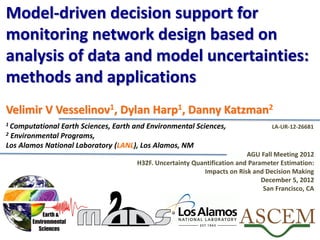
  • 81. 2009 model estimate of the plausible contaminant concentrations [ppb] along the regional aquifer water table  Wells R-62, R-61 and R-50 were not drilled yet  Locations of wells R-62, R-61 and R-50 were optimized based on model analyses  Observed concentrations at R-62, R-61 and R-50 confirmed model predictions  R-43 concentration were at background when the analyses were performed  Since 2010, R-43 concentrations are increasing and approaching the model predicted concentration MCL = 50 ppb
  • 82. 2009 model estimate of the plausible contaminant concentrations [ppb] along the regional aquifer water table  Wells R-62, R-61 and R-50 were not drilled yet  Locations of wells R-62, R-61 and R-50 were optimized based on model analyses  Observed concentrations at R-62, R-61 and R-50 confirmed model predictions  R-43 concentration were at background when the analyses were performed  Since 2010, R-43 concentrations are increasing and approaching the model predicted concentration 100 ~30-200 MCL = 50 ppb 18
  • 83. 2009 model estimate of the plausible contaminant concentrations [ppb] along the regional aquifer water table  Wells R-62, R-61 and R-50 were not drilled yet  Locations of wells R-62, R-61 and R-50 were optimized based on model analyses  Observed concentrations at R-62, R-61 and R-50 confirmed model predictions  R-43 concentration were at background when the analyses were performed  Since 2010, R-43 concentrations are increasing and approaching the model predicted concentration 100 ~30-200 MCL = 50 ppb ~40 18
  • 84. MADS is applied to perform all the presented info-gap decision analyses …
  • 85.  an open-source high-performance computational framework for analyses and decision support based on complex process models  advanced adaptive computational techniques: o sensitivity analysis (local / global); o uncertainty quantification (local / global); o optimization / calibration / parameter estimation (local / global); o model ranking & selection o decision support (GLUE, info-gap)  novel algorithms o Agent-Based Adaptive Global Uncertainty and Sensitivity (ABAGUS) Harp & Vesselinov (2012) An agent-based approach to global uncertainty and sensitivity analysis. Computers & Geosciences. o Adaptive hybrid (local/global) optimization strategy (Squads) Vesselinov & Harp (2012) Adaptive hybrid optimization strategy for calibration and parameter estimation of physical process models. Computers & Geosciences.  internal coupling with analytical contaminant transport solvers and test problems  external coupling with existing process simulators (ModFlow, TOUGH, FEHM, eSTOMP, Amanzi, …)  Source code, examples, performance comparisons, and tutorials @ http://mads.lanl.gov
  • 86. Advanced Subsurface Computing for Environmental Management  an open-source interactive decision support system (Akuna/Agni) coupled a process simulator (Amanzi)  high-performance computing (HPC)  data- and model-driven decision support to provide standardized, consistent, site-specific and scientifically defensible decision analyses across DOE-EM complex  Challenge: o develop tools to make better use of complex information and capabilities to explore problems in greater detail o address the most challenging performance assessment and waste-disposal problems  Impact: o provide technical underpinnings for current U.S. DOE-EM risk and performance assessments o inform strategic data collection for model improvement and decision support o support scientifically defensible and standardized assessments and remedy selections Regulatory Public Interface Reviews Decision Making Scientific Model Setup and Execution Model Analyses Decision Support Programmatic Project Management Oversight Decision Making http://ascemdoe.org
  • 87. AMANZI AKUNA AGNI Modules Akuna (“no worries”): Graphic User Interface (Karen Schuchardt, PNNL) • Open Source Eclipse/Java based • Incorporates data management, visualization, and model development tools Agni (“fire”): Simulation controller and Toolset driver (George Pau, LBNL, Velimir Vesselinov, LANL) • Open Source C++ object oriented • Provides coupling between Akuna and Amanzi • Performs various model-based analyses (SA, UQ, PE, DS, … ) Amanzi (“water”): HPC Flow and Transport Simulator (David Moulton, LANL) • Open Source C++ object oriented • Saturated / unsaturated groundwater flow, … • Structured / unstructured / adaptive gridding • … http://ascemdoe.org
  • 88. Model-Analysis Toolsets in Agni o Sensitivity Analysis (SA) (Stefan Finsterle, Elizabeth Keating) o Parameter Estimation (PE) (Stefan Finsterle, LBNL) o Uncertainty Quantification (UQ) (Elizabeth Keating, LANL) o Risk Assessment (RA) (Wilson McGinn, ORNL) o Decision Support (DS) (Velimir Vesselinov, LANL) http://ascemdoe.org
  • 89. Conclusions and recommendations:  Both Non-Probabilistic and Probabilistic uncertainties often exist in a decision problem  Non-Probabilistic and Probabilistic methods should be applied to their appropriate uncertainties in the decision analyses  In the case of probabilistic methods, definition of prior probability distributions for model parameters or calibration targets with unknown/uncertain distribution can produce biased predictions and decision analyses  In the case of non-probabilistic methods, lack of knowledge and severe uncertainties can be captured  Non-probabilistic methodologies have been successfully applied for a series of synthetic and real-world problems, though less often in hydrology o Remediation of unknown contaminant source Harp & Vesselinov (2011). Contaminant remediation decision analysis using information gap theory. SERRA  MADS provides a computationally efficient framework for decision analyses using non-probabilistic and probabilistic methods ( http://mads.lanl.gov )  ASCEM tools are currently actively developed and will become available for testing and benchmarking in 2013 ( http://ascemdoe.org )