Introduction to Relational Algebra and Advanced SQL.pdf

1. Lecture 5 Relational Algebra
and Advanced SQL
Ming-Ling Lo
20220321

2. Overview of
Relational Algebra
2

3. Operations in a Data Model
● A complete data model must cover the following aspects:
○ Structure of data
○ Constraints on data
○ Operations on data
● ER model and Relational Data Model cover the first two
● Relational Algebra and Relational Calculus
○ Formally specify the operations on relational data
3

4. Relational Calculus and Relational Algebra
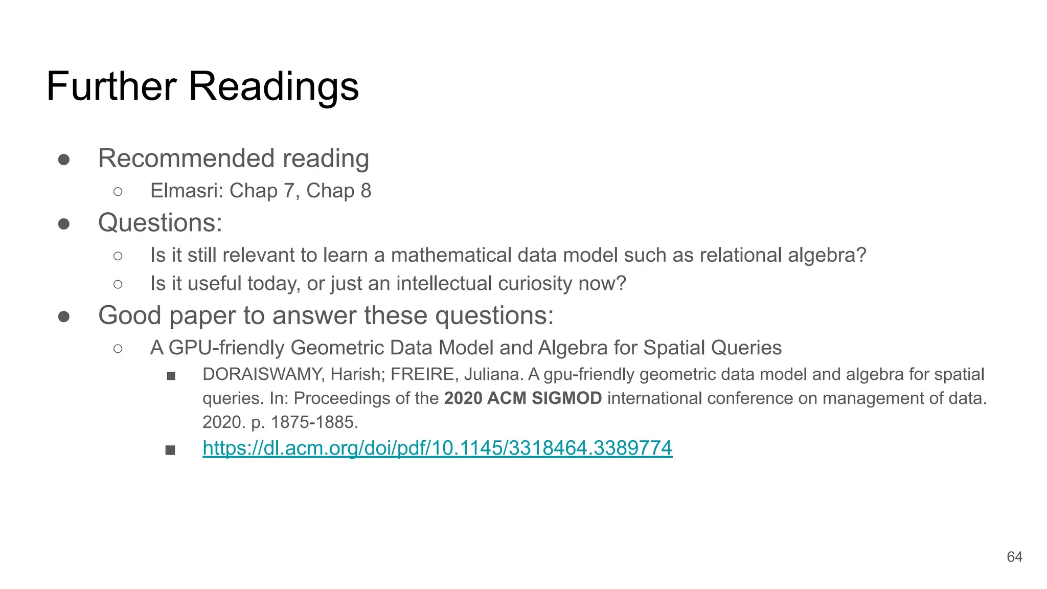
● Relational Calculus and relational algebra
○ Both originally proposed by Edgar F. Codd in the early 1970s
○ Formally specify operations on relational data
○ Logically equivalent: Any query specified in r. calculus can be specified in r. Algebra; vice versa
● Relational calculus
○ Tuple relational calculus: proposed Edgar F. Codd 1971
○ Domain relational calculus: proposed by by Michel Lacroix and Alain Pirotte 1977
○ Both are based on 1st order predicate logic (and set operations)
● Tuple Relational Calculus (TRC)
○ Specify what the tuples satisfied the conditions to be selected
○ Examples::
■ {t | t ∈ Employee and t[SALARY] > 60,000 }
● Equivalent to relational algebra: T ← σ SALARY> 60,000
(EMPLOYEE)
■ {t | ∃ r ∈ EMPLOYEE ( t[NAME] = r[NAME] ^ r[SALARY] > 60,000) }
● Equivalent to relational algebra: ΠNAME
( σ SALARY> 60,000
(EMPLOYEE))
4

5. Relational Algebra
● What is an algebra (in the sense of mathematical abstract algebra)?
○ A set along with some number of operations
○ The set is “closed under the operations” and the operations satisfy certain properties
○ Algebraic structures include: group, semigroup, ring, field, vector space, …, etc.
● Relation algebra:
○ A field of mathematic study, emerged in the 19th-century work of Augustus De Morgan and Charles Peirce, etc.
● Relational algebra
○ Defined as an “algebra” in rigorous mathematical sense, by Edgar F. Codd for relational database operations
○ Relations are closed under relational algebra operations: RA
op RB
= RC
● Why important?
○ Theoretical aspect:
■ Provides a formal foundation for operations in relational model
■ Provides a theoretical basis for definition and development of SQL as a language
○ Practical aspect:
■ Help us fully grasp (complicated) SQL operations
■ Used as a basis in query processing and optimization
● Query processing and optimization is an important aspect in RDBMS operation
5

6. Relational Algebra Operations
● Can be divided into:
○ Operations from mathematical set theory
■ UNION
■ INTERSECTION
■ SET DIFFERENCE
■ CARTESIAN PRODUCT (also known as CROSS PRODUCT).
○ Operations developed specifically for relational databases
■ SELECT, PROJECT
■ RENAME
■ JOIN, Division
■ Aggregate functions
■ OUTER JOINS, OUT UNIONS
● Can also be divided into:
○ Unitary operations
○ Binary operations
6

7. Operations in
Relational Algebra
7

8. Unary Relational Operations - Select
● SELECT
○ Choose a subset of the tuples from a relation that satisfies a selection condition
○ Result is another relation
○ Horizontal partition of the relation into two sets
■ Tuples that satisfy the condition -- selected
■ Tuples that do not satisfy the condition -- discarded
● Syntax: R’ = σ<selection condition>
(R)
○ Symbol σ (sigma) is used to denote the SELECT operator
○ <selection condition> is a Boolean expression specified on the attributes of relation R
● E.g.
○ σDno=4
(EMPLOYEE)
○ σSalary>30000
(EMPLOYEE)
8

9. Unary Relational Operations - Select (2)
● <selection condition>
○ Not <Clause>
○ <Clause> and/or <clause>
○ <Clause> and/or <selection condition>
● <clause>
○ <attribute name> <comparison op> <constant value>
○ <attribute name> <comparison op> <attribute name>
● <comparison op>
○ one of the operators {=,<,≤,>,≥,≠}
● Selection operation is applied to each tuple individually
○ Hence, selection conditions cannot involve more than one tuple
9

10. Properties of Select
● Assume R’ = σ<selection condition>
(R)
● The degree of R’ is the same as the degree of R.
● The cardinality of R’ is always less than or equal to the cardinality of R
○ I.e., |R’| ≤ |R|
● Selectivity of the selection operation:
○ Ratio of tuple selected = |R’| / |R|
● SELECT operation is commutative
○ σ<cond1>
(σ<cond2>
(R)) = σ<cond2>
(σ<cond1>
(R))
○ Sequence of SELECTs can be applied in any order
● We can always combine a sequence of SELECT operations into a single
SELECT operation
○ σ<cond1>
(σ<cond2>
(...(σ<condn>
(R)) ...)) = σ<cond1> AND<cond2> AND...AND <condn>
(R)
10
select

11. Select and SQL
● In SQL, the SELECT condition is typically specified in the WHERE clause
● For example,
σDno=4 AND Salary>25000
(EMPLOYEE)
→
SELECT *
FROM EMPLOYEE
WHERE Dno=4 AND Salary>25000;
11

12. Unary Relational Operation - Project
● PROJECT
○ Selects certain columns from the table and discards the other columns.
○ The output is also a relation
○ Vertical partition of the relation into two relations
■ One with the needed columns (attributes) -- result of project
■ One with unwanted columns -- discarded
● Syntax: R’ = π<attribute list>
(R)
○ π(pi) is the symbol used to represent the PROJECT operation
○ <attribute list> is the list of desired attributes from the attributes of relation R
○ Order of attributes in R’ is the same as they appear in <attribute list>.
● E.g.
○ πLname, Fname, Salary
(EMPLOYEE)
12

13. Properties of Project
● Assume R’ = π<attribute list>
(R) <attribute list>
● If <attribute list> does not include a key of R, duplicate tuples may occur
○ In relational algebra, by definition , PROJECT removes any duplicate tuples
○ That is, the result of PROJECT is a set of distinct tuples, and a valid relation.
○ In SQL, it is allowed not to remove duplicates, i.e., the result may be a multiset or a set
● The degree of R’ = the number of attributes in <attribute list>
○ Degree of R’ <= degree of R
● The cardinality of R’ <= the cardinality of R
○ That is, |R’| = |π<attribute list>
(R)| <= |R|
○ If <attribute list> is a superkey of R, then
|R’| = |π<attribute list>
(R)| = |R|
13

14. ● If <list2> contains the attributes in <list1>, then
π<list1> (π<list2>(R)) = π<list1>(R)
○ Otherwise, π<list1> (π<list2>(R)) is an incorrect expression.
● Commutativity does not hold on PROJECT
Properties of Project (2)
14

15. Project and SQL
● πSex, Salary
(EMPLOYEE) corresponds to the following SQL query
→
SELECT DISTINCT Sex, Salary
FROM EMPLOYEE
Think (open question):
1. In current relational algebra, attribute list in “project” is given as
constant. Can relational algebra be extended so that the attribute
list is the result of some condition or the result of some other
relational algebra operation?
15

16. Unary Relational Operation - Rename
● RENAME
○ Rename relations and attributes
○ Useful when writing complex relational expressions
■ Improve readability: clearly specifying which attributes of which relation
■ Enable writing certain operations which are otherwise difficult to express
● Syntax: ρS(B1, B2, ..., Bn)
(R)
○ ρ(rho) is the symbol used to denote the RENAME operator
○ S is the new relation name, and B1, B2, ..., Bn are the new attribute names
○ Simplified forms:
■ ρS
(R): rename only the relation R to S
■ ρ(B1, B2, ..., Bn)
(R): rename only the attributes of R to B1, B2, … Bn
16

17. Rename and SQL
● Renaming in SQL is accomplished by AS
● The following SQL statement is the combination of a rename and a select
→
SELECT E.Fname AS First_name, E.Lname AS Last_name, E.Salary AS Salary
FROM EMPLOYEE AS E
WHERE E.Dno=5,
17

18. Set Operations and Union Compatibility
● Union compatibility
○ Important concept when talking about set operations on relations
● Two relations R(A1,A2,...,An) and S(B1,B2,...,Bn) are said to be union
compatible (or type compatible) if
○ R and S have the same degree n
○ dom(Ai) = dom(Bi) for 1 ≤ i ≤ n
● Set operations can be done on all pairs of relations, but are meaningful only
used upon relations of union compatibility
● For set operations in RDB, we adopt the convention that the resulting relation
has the same attribute names as the first relation R
18
//ie. need to have same attributes and in same order to be unionable

19. Set Operations
● Assume R and S are union compatible
● UNION: R ∪ S
○ Result is a relation that includes all tuples that are either in R or in S, or in both R and S.
Duplicate tuples are eliminated.
● INTERSECTION: R ∩ S
○ Result is a relation that includes all tuples that are in both R and S.
● SET DIFFERENCE (or MINUS): R – S
○ Result is a relation that includes all tuples that are in R but not in S.
19

20. Properties of Set Operations
● UNION and INTERSECTION are commutative operations
R ∪ S = S ∪ R
R ∩ S = S ∩ R
● UNION and INTERSECTION can be treated as n-ary operations applicable to
any number of relations because both are also associative operations; that is,
R ∪ (S ∪ T)=(R ∪ S) ∪ T and (R ∩ S) ∩ T = R ∩ (S ∩ T )
● The MINUS operation is not commutative; that is, in general,
R − S ≠ S − R
20

21. Properties of Set Operations (2)
● INTERSECTION can be expressed in terms of union and set difference as
follows:
R ∩ S = (R ∪ S) − (R − S) − (S − R)
● In SQL, the corresponding operations are
○ UNION,INTERSECT,and EXCEPT
● In addition, there are multiset versions these set operations:
○ UNION ALL, INTERSECT ALL, and EXCEPT ALL
■ Do not eliminate duplicates
21

22. Properties of Set Operations
● In practice, some DBMS implements only the UNION operations
○ Can all set operations be expressed such DBMS? Yes (why?)
● The following SQL statement takes union of two type-compatible tables
→
SELECT * from EE_STUDENTS
UNION
SELECT * from MATH_STUDENTS;
TABLE EE_STUDENTS
UNION
SELECT * from MATH_STUDENTS;
TABLE EE_STUDENTS
UNION
TABLE MATH_STUDENTS;
22
Think:
1. Why need union compatibility?
What will happen if there is no
union compatibility?
2. Can you define a set of set
operations without union
compatibility?

23. Binary Operation: Cartesian Product
● CARTESIAN PRODUCT
○ Also known as cross product
○ Generate a big relation with tuples formed by combining two input relations
○ Same as the cartesian product in mathematical sense
○ Not particularly useful in practice, but very useful as a concept to understand JOIN operation
● Syntax and definition: Q = R(A1, A2, ...,An) × S(B1, B2, ...,Bm)
○ Q has one tuple for each combination of tuples—one from R and one from S
● Properties
○ The degree of Q = n + m. That is, Q = Q(A1, A2, ...,An, B1, B2, ...,Bm)
○ If R has nR tuples and S has nS tuples, then R×S will have nR * nS tuples.
That is, |R×S| = |R| × |S|
23

24. Binary Operation: Join
● JOIN
○ The most important operation in relational database
○ Allows us to process relationships among relations
● Syntax: Q = R ⨝<join condition>
S
○ The JOIN operation is denoted by ⨝ here
○ Used to combine related tuples from two relations into single “longer” tuples.
■ Q has one tuple for each combination of tuples—one from R and one from S—whenever
the combination satisfies the join condition
○ Assume R(A1, A2, ...,An) and S(B1, B2,...,Bm), join of R and S can also be denoted more
explicitly as
Q(A1,A2,...,An, B1,B2,...,Bm) = R(A1,A2, ...,An) ⨝<join condition>
S(B1,B2, ...,Bm)
● E.g.
○ Find the name of manager for each department
DEPT_MGR ← DEPARTMENT ⨝Mgr_ID=ID
EMPLOYEE
RESULT ←πDname, Lname, Fname
(DEPT_MGR)
⨝
24
step 1: a Cartesian product
step 2: only SELECT wanted attributes
:=
JOIN:

25. Join Operation (2)
● The JOIN operation can be considered as a CARTESIAN PRODUCT followed
by a SELECT
● In the previous example:
○ DEPT_MGR ← DEPARTMENT ⨝Mgr_ID=ID
EMPLOYEE
==
DEPT_MGR ← σ<Mgr_ID=ID>
(DEPARTMENT × EMPLOYEE)
● Main difference between CARTESIAN PRODUCT and JOIN.
○ In JOIN, only combinations of tuples satisfying the join condition appear in the result
○ In the CARTESIAN PRODUCT all combinations of tuples are included in the result.
25

26. Join Conditions
● The join condition is
○ Specified on attributes from the two relations R and S
○ Evaluated for each combination of tuples.
○ Each tuple combination for which the join condition evaluates to TRUE is included in the resulting
relation Q as a single combined tuple.
○ Tuple combinations that include NULL or for which the join condition is FALSE do not appear in the
result
● A general join condition is of the form
<condition> AND <condition> AND...AND <condition>
where each <condition> is of the form Ai θ Bj,
Ai is an attribute of R,
Bj is an attribute of S,
Ai and Bj have the same domain, and
θ (theta) is one of the comparison operators {=, <, ≤, >,≥, ≠}.
26

27. Join Selectivity
● Join selectivity:
○ Ratio of the cardinality of the join result and the cartesian product of the input relations
○ Assume, R has nR tuples, and S has nS tuples, and Q = R ⨝ S
Join selectivity = |R ⨝ S| / (|R| * |S|)
= |Q| / (|R| * |S|)
= |Q| / (nR * nS)
● In DBMS implementations, we often need to estimate the join selectivity without
actually executing the join (even before the data is completely collected/updated)
○ So often when we say “join selectivity” we are referring to the expected join selectivity, that is:
Join selectivity = E( |Q| / |R| * |S| )
● Properties:
○ The result of a JOIN operation R ⨝ S will have between zero and nR * nS tuples.
○ If there is no join condition, all combinations of tuples qualify, and the JOIN degenerates into a
CARTESIAN PRODUCT ⇒ Join selectivity = 1
○ If no combination of tuples satisfies the join condition, the result is an empty relation ⇒ Join selectivity
= 0
27

28. ● THETA JOIN
○ A JOIN operation with a general join condition is called a THETA JOIN
● EQUIJOIN
○ In <join condition>, only = is used
○ One of most frequently used join operation
● Natural Join
○ The most important join. The most commonly used JOIN
○ Similar to equijoin, but
■ Remove one of the join attribute from each join attribute pairs
■ Requires that the two join attributes (or each pair of join attributes) have the same name
in both relations.
● If this is not the case,a renaming operation is applied first.
Theta Join, Equijoin, and Natural Join
28
These names appear in
the literature frequently
// joining attributes have same name

29. More on Natural Join
● Syntax: Q = R * S
○ Use * as symbol
● E.g. assume PROJECT has an attribute Dnum
○ PROJ_DEPT ← PROJECT * ρ(Dname, Dnum, Mgr_ssn, Mgr_start_date)
(DEPARTMENT)
○ Or, equivalently
DEPT ←ρ (Dname, Dnum, Mgr_ssn, Mgr_start_date)
(DEPARTMENT)
PROJ_DEPT ← PROJECT * DEPT
● E.g. assume DEPT and DEPT_LOC both have attribute Dnum
○ DEPT_LOCS ← DEPT * DEPT_LOC
29

30. Semijoin
● SEMIJOIN
○ Similar to the natural join, but with certain columns excluded
○ Include left semijoin and right semijoin.
○ The left semijoin is the set of all tuples in R for which there is a tuple in S that is equal on their
common attribute names. The difference from a natural join is that other columns of S do not
appear. The right semijoin is also defined similarly, but with the role of R and S exchanged.
● Syntax: R ⋉ S (left semijoin) or R ⋊ S (right semijoin)
○ Use ⋉ and ⋊ as symbols
● Properties
○ The semijoin can be simulated using the natural join as follows.
■ Assume a1, ..., an are the attribute names of R, then
R ⋉ S = π a1,..,an
(R * S).
○ Note: In Codd's 1970 paper, semijoin is called restriction.
30
The term semijoin also
appears in the literature
frequently
eg. just want tuples in R that appear in S

31. Antijoin
● ANTIJOIN
○ The antijoin between R and S is similar to the semijoin, but includes as result only those tuples
in R for which there is no tuple in S with an equal value on their common attribute names
● Syntax: R ▷ S
○ Use ▷ as symbol
● Properties:
○ The antijoin can also be defined as the complement of the semijoin, i.e.:
R ▷ S = R − R ⋉ S
○ Given this, the antijoin is sometimes called the anti-semijoin, and the antijoin operator is
sometimes written as semijoin symbol with a bar above it, instead of ▷
31
The term antijoin occasionally
appears in the literature

32. Division
● The DIVISION is denoted by ÷
● Can be seen as the “inverse” of cartesian product
● Useful when answering question with “ALL”
A B
a1 b1
a2 b1
a1 b2
a2 b2
a3 b2
A
a1
a2
÷ =
B
b1
b2
A B
a1 b1
a2 b1
a1 b2
a2 b3
a3 b2
A
a1
a2
÷ =
B
b1
32

33. Division
● Note:
○ When DIVISION operation is applied to two relations T = R ÷ S,
their attributes must have the following relationship T(Y) = R(Z) ÷ S(X),
where X ⊆ Z, and Y = Z – X (and Z = X ∪ Y).
● E.g.
○ Retrieve the names of employees who work on all the projects that ‘John Smith’ works on.
SMITH ←σ
Fname=‘John’ AND Lname=‘Smith’
(EMPLOYEE)
SMITH_PNOS ←π
Pno
(WORKS_ON ⋈EID=Smith.ID
SMITH)
ID_PNOS ←π
EID, Pno
(WORKS_ON)
SID(ID) ← ID_PNOS ÷ SMITH_PNOS
RESULT ←π
Fname, Lname
(SID * EMPLOYEE)
33
Ex: look for tuples who have same attributes as target divisee

34. Complete Set of Relational Algebra Operations
● Complete set of relational algebra operations: {σ,π,∪,ρ, –,×}
● The following operations, though important, are not fundamental
○ Intersection: R ∩ S ≡ (R ∪ S) – ((R – S) ∪ (S – R))
○ Jion: R ⨝ <condition>
S ≡ σ<condition>
(R × S)
○ Division:
Assume we have relation R(Z), and Z = X ∪ Y, where Y is the attribute on which we want to
ask the question, the division T(Y) ← R(Z) ÷ S(X) can be expressed as a sequence of π,×,and
– operations as follows:
T1 ←πY
(R)
T2 ←πY
((S × T1) – R)
T ← T1 – T2
34
Example: assume R(proj, person), S(person)
T1: all projects
S×T1: the combination of all projects and people
(S × T1) – R: (proj, person) combination that do not exist in R;
T2: proj that are not participated by all people in S
T: proj that are participated by all people in S

35. Additional Relational Operations
● Not in original relational algebra definition
● Included for convenience
● Including
○ Generalize projection
○ Recursive closure
○ Aggregate functions and grouping (important)
○ Outer join (important, for practical reasons)
○ Outer union
35

36. Generalized Projection
● Generalized Projection
○ Allow functions on attributes as project attributes
○ π F1, F2, ..., Fn
®
● E.g. Calculate Employee’s net salary
REPORT ←
ρ (Ssn, Net_salary, Bonus, Tax)
( πSsn, Salary – Deduction, 2000 * Years_service, 0.25 *
Salary
(EMPLOYEE))
36

37. Recursive Closure
● Example:
Find out supervisors of all employees recursively
● If we fix level N, we can always get answers
● If we do not know N, it cannot be implemented in the original Relational
Algebra definition
● An operation called transitive closure has been proposed (syntax included in
SQL3)
37

38. Aggregate Functions and Grouping
● Find out summary information for each “group” of tuples in a relation
● Syntax
<grouping attributes>
ℑ <function list>
(R)
● For each department, find out number of employees, and their average salary
Dno
ℑ COUNT Ssn, AVERAGE Salary
(EMPLOYEE)
● For all employee (in the company), find out total number of employees, and
average salary
ℑ COUNT Ssn, AVERAGE Salary
(EMPLOYEE)
● Aggregate functions
SUM, AVERAGE, MAXIMUM, MINIMUM,COUNT
38
Important

39. Outer Join
● “Those tuples not selected by JOIN conditions are also kept”
● Three types
○ Left outer join
○ Right outer join
○ Full outer join
39
Important

40. Outer Join (2)
No
match
match
match
No
match
No
match
NULL
match match
R S
Left out join
match match
NULL No
match
Right outer join
Full outer join
No
match
NULL
match match
match match
NULL No
match
match match
Theta join
40

41. Outer Union
● Union between two relations that have some, but not all, attributes in common
● Effect: The same as a FULL OUTER JOIN on the common attributes.
● Assume two relations R(X, Y) and S(X, Z) where attributes X, are union compatible
● Form: The outer union is of the form T(X, Y, Z) = Outer_union(R(X, Y), S(X, Z),
○ Note: the attributes that are union compatible are represented only once in the result, and those attributes that are not union
compatible, i.e., Y and Z, from either relation are also kept in the result relation T(X, Y, Z).
● Content:
○ Tuples t1 in R and t2 in S are said to match if t1[X] = t2[X]
○ Matched tuples will be combined into a single tuple in the result relation T, by taking Y from R and Z from S.
○ Tuples in R or S that have no match are padded with NULL values, and also put into the union.
● For example
○ OUTER UNION between two relations
■ STUDENT(Name, Ssn, Department, Advisor) and INSTRUCTOR(Name, Ssn, Department, Rank)
■ will be STUDENT_OR_INSTRUCTOR(Name, Ssn, Department, Advisor, Rank)
○ All the tuples from both relations are included in the result,
○ Tuples with the same (Name, Ssn, Department) combination will appear only once in the result.
○ Tuples appearing only in STUDENT will have a NULL for the Rank attribute,
○ Tuples appearing only in INSTRUCTOR will have a NULL for the Advisor attribute.
○ A tuple that exists in both relations, which represent a student who is also an instructor, will have values for all its attributes.
41

42. Advanced SQL
and Complex Queries
42

43. Select and NULL
● SQL allows one to select tuples with NULL values
● But with special operators IS and IS NOT
● Example
○ SELECT Fname, Lname
FROM EMPLOYEE
WHERE Super_ssn IS NULL;
● Note: we must say “IS NULL”, not “= NULL”
○ SQL consider every NULL to be different from other NULL
43

44. Three-Valued Logic
● TRUE + FALSE + UNKOWN ⇒ Three-valued logic
● Recap: NULL can mean
○ Unknow: Not know whether exist, and not know the value
○ Unavailable: value exists but not available to us
○ Not applicable
● Why important? It will appears in SQL statements
AND TRUE FALSE
TRUE TRUE FALSE
FALSE FALSE FALSE
AND TRUE FALSE UNKNOWN
TRUE TRUE FALSE UNKNOWN
FALSE FALSE FALSE FALSE
UNKNOWN UNKNOWN FALSE UNKNOWN
44

45. Three-Valued Logic (2)
● Why important?
● In Select...From...Where queries, only tuple which evaluated to be TRUE are
selected
○ Tuples evaluated to be unknown (NULL) are not selected
OR TRUE FALSE UNKNOWN
TRUE TRUE TRUE TRUE
FALSE TRUE FALSE UNKNOWN
UNKNOWN TRUE UNKNOWN UNKNOWN
NOT
TRUE FALSE
FALSE TRUE
UNKNOWN UNKNOWN
45

46. Renaming of Relations and Attributes (Alias)
● In SQL, it is possible to rename attributes that appear in the query result
(appears after the SELECT keyword)
● It is possible to rename relations that appear in the FROM clause
● Use the qualifier AS, followed by the desired new name.
○ The AS construct can be used to rename both attribute and relation names
● For example
SELECT E.Lname AS Employee_name, S.Lname AS Supervisor_name
FROM EMPLOYEE AS E, EMPLOYEE AS S
WHERE E.Super_ssn=S.Ssn;
46
Scope: the query only

47. Join Operation in SQL
● SELECT Fname, Lname, Address
FROM EMPLOYEE, DEPARTMENT
WHERE Dname=‘Research’ AND Dnumber=Dno;
● SELECT Pnumber, Dnum, Lname, Address, Bdate
FROM PROJECT, DEPARTMENT, EMPLOYEE
WHERE Dnum=Dnumber AND Mgr_ssn=Ssn AND Plocation=‘Taipei’;
Join attributes
Join attributes
47

48. Union in SQL
● (SELECT DISTINCT Pnumber
FROM PROJECT, DEPARTMENT, EMPLOYEE
WHERE Dnum=Dnumber AND Mgr_ssn=Ssn AND Lname=‘Smith’)
UNION
( SELECT DISTINCT Pnumber
FROM PROJECT, WORKS_ON, EMPLOYEE
WHERE Pnumber=Pno AND Essn=Ssn AND Lname=‘Smith’);
● UNION, INTERSECT, EXCEPT (set difference)
○ Not all DBMS’s support all of them. But their function can usually be obtained by other means
48

49. Complex Queries
● Nested queries
● Joined tables
● Outer joins
● Aggregate functions
● Grouping
49

50. IN Operator
● Test whether a value is in a set
○ Can use explicit set value
○ Can use dynamic set value to form nested queries
SELECT DISTINCT Essn
FROM WORKS_ON
WHERE Pno IN (1, 2, 3);
50
This set can be dynamically
generated (see next page)

51. Nested Queries using IN Operator
● Use dynamic set value in IN comparison
● SELECT att1, att2
FROM table1
WHERE att3 in ‘some set’
● We can construct this set dynamically
○ The answer of a query is another relation
○ Relation is a set
● SELECT att1, att2
FROM table1
WHERE att3 in
(SELECT att4
FROM table2
WHERE att5 = val)
51
att3 and att4 must be
domain-compatible, of
course !
SELECT DISTINCT Emp_ID
FROM WORKS_ON
WHERE (Pno, Hours) IN ( SELECT Pno, Hours
FROM WORKS_ON
WHERE Emp_ID=‘123456’)
and Hours >= 20;
Can have multiple
attributes here

52. ● Multiple dynamic sets can be unioned together using “or” in a nested query
● Some effect as union
SELECT DISTINCT Pname, Pleader
FROM PROJECT
WHERE Pnumber IN
(SELECT Pnumber
FROM PROJECT, DEPARTMENT, EMPLOYEE
WHERE Dnum=Dnumber AND Mgr_ssn=Ssn AND Lname=‘Smith’)
OR
Pnumber IN
(SELECT Pno
FROM WORKS_ON, EMPLOYEE
WHERE Essn=Ssn AND Lname=‘Smith’ );
Nest Queries with OR
Two dynamic sets unioned together with “or”
52

53. Nest Queries and Set Member Comparison Operators
● Ordinary comparison operators
○ Determine whether an element qualify based on its relationship another element or value
○ =, >, <, >=, <= <>
○ E.g. a=2, b>c. Etc.
● Set member comparison operators
○ Determine whether an element qualify based on its relationship to a set
○ IN
○ ‘=, >, <, >=, <=’ combined with ‘SOME, ANY, ALL’
○ E.g. ‘=SOME’, ‘>ALL’
○ Note:
■ SOME and ANY have the same effect
■ =SOME and =ANY have the same effect as IN
53

54. Nest Queries with SOME and ALL
SELECT Lname, Fname
FROM EMPLOYEE
WHERE Salary > ALL ( SELECT Salary
FROM EMPLOYEE
WHERE Dno=5 );
54
SELECT Lname, Fname
FROM EMPLOYEE
WHERE Lname=SOME (SELECT Lname
FROM EMPLOYEE
WHERE Dno=5 );
Lname IN

55. Nest Queries and Relation Alias
● Give ‘Alias’ to a relations in the query, so that we know clearly which relations
we are talking about
● When two relations may use the same attribute names, alias becomes
necessary
SELECT E.Fname, E.Lname
FROM EMPLOYEE AS E
WHERE E.Ssn IN ( SELECT Essn
FROM DEPENDENT AS D
WHERE E.Fname=D.Dependent_name AND
E.Sex=D.Sex );
Is this important?
55

56. Correlated Nested Queries
● When a condition in the WHERE clause of a nested query references
some attribute of a relation declared in the outer query, the two queries
are said to be correlated.
● What’s special about correlated?
○ The nested query is evaluated once for each tuple (or combination of tuples) in the outer query
⇒ expensive!
SELECT E.Fname, E.Lname
FROM EMPLOYEE AS E
WHERE E.Ssn IN (
SELECT Essn
FROM DEPENDENT AS D
WHERE E.Fname = D.Dependent_name
AND E.Sex=D.Sex );
An exemplary way to implement the query:
For each EMPLOYEE tuple, evaluate the nested
query, which retrieves the Essn values for all
DEPENDENT tuples with the same sex and first
name as those of the EMPLOYEE tuple; if the
Ssn value of the EMPLOYEE tuple is in the result
of the nested query, then select that EMPLOYEE
tuple. 56

57. Nested Queries Flattening
● In general, a query written with nested select-from-where blocks and using
the = or IN comparison operators can always be expressed as a single block
query
SELECT E.Fname, E.Lname
FROM EMPLOYEE AS E, DEPENDENT AS D
WHERE E.Ssn=D.Essn AND
E.Fname=D.Dependent_name AND
E.Sex=D.Sex
SELECT E.Fname, E.Lname
FROM EMPLOYEE AS E
WHERE E.Ssn IN (
SELECT Essn
FROM DEPENDENT AS D
WHERE
E.Fname = D.Dependent_name
AND E.Sex=D.Sex );
57

58. Exist
● The EXISTS function in SQL is used to check whether the result of a correlated nested
query is empty or not.
● The result of EXISTS is a Boolean value TRUE if the nested query result contains at
least one tuple, or FALSE if the nested query result contains no tuples.
SELECT E.Fname, E.Lname
FROM EMPLOYEE AS E
WHERE EXISTS (
SELECT *
FROM DEPENDENT AS D
WHERE E.Ssn=D.Essn );
SELECT Fname, Lname
FROM EMPLOYEE AS E
WHERE NOT EXISTS (
SELECT *
FROM DEPENDENT AS D
WHERE E.Ssn=D.Essn );
58

59. Joined Tables
● Provided as convenient mechanism
● The following three select statements are the same:
● SELECT Fname, Lname, Address
FROM EMPLOYEE, DEPARTMENT
WHERE Dname=‘Research’ AND Dnumber=Dno
● SELECT Fname, Lname, Address
FROM (EMPLOYEE JOIN DEPARTMENT ON Dno=Dnumber)
WHERE Dname=‘Research’;
● SELECT Fname, Lname, Address
FROM (EMPLOYEE NATURAL JOIN
(DEPARTMENT AS DEPT (Dname, Dno, Mssn, Msdate)))
WHERE Dname=‘Research’;
59
You are encouraged to
use pure select as much
as possible (without using
the join operator)

60. Outer Join
● SELECT E.Lname AS Employee_name, S.Lname AS Supervisor_name
FROM (EMPLOYEE AS E LEFT OUTER JOIN
EMPLOYEE AS S
ON E.Super_ssn=S.Ssn);
● Same for
○ LEFT OUTER JOIN
○ RIGHT OUTER JOIN
○ FULL OUTER JOIN
60

61. Aggregate Functions
● COUNT, SUM, MAX, MIN, and AVG
● SELECT SUM (Salary), MAX (Salary), MIN (Salary), AVG (Salary)
FROM EMPLOYEE;
● SELECT COUNT (*)
FROM EMPLOYEE;
● SELECT COUNT (DISTINCT Salary)
FROM EMPLOYEE;
61

62. Group By and Having
● SELECT Dno, COUNT (*), AVG (Salary)
FROM EMPLOYEE
GROUP BY Dno;
● SELECT Pnumber, Pname, COUNT (*)
FROM PROJECT AS P, WORKS_ON AS W
WHERE P.Pnumber=W.Pno
GROUP BY P.Pnumber, P.Pname;
● SELECT Pnumber, Pname, COUNT (*)
FROM PROJECT, WORKS_ON WHERE Pnumber=Pno
GROUP BY Pnumber, Pname
HAVING COUNT (*)>2;
62
● Important!
● Aggregate functions in
combination with group by, having
⇒ Very useful and powerful for data
preprocessing (In data analysis,
data science, machine learning, …
etc.)
//outputs Pnumber x Pname’s count

63. Modern Aggregate
Functions
Name Description
AVG() Return the average value of the argument
BIT_AND() Return bitwise AND
BIT_OR() Return bitwise OR
BIT_XOR() Return bitwise XOR
COUNT() Return a count of the number of rows returned
COUNT(DISTINCT) Return the count of a number of different values
GROUP_CONCAT() Return a concatenated string
JSON_ARRAYAGG() Return result set as a single JSON array
JSON_OBJECTAGG() Return result set as a single JSON object
MAX() Return the maximum value
MIN() Return the minimum value
STD() Return the population standard deviation
STDDEV() Return the population standard deviation
STDDEV_POP() Return the population standard deviation
STDDEV_SAMP() Return the sample standard deviation
SUM() Return the sum
VAR_POP() Return the population standard variance
VAR_SAMP() Return the sample variance
VARIANCE() Return the population standard variance
● Using MySQL as example
63
You can also add your own
aggregate functions into MySQL
(https://dev.mysql.com/doc/extendi
ng-mysql/8.0/en/)

64. Further Readings
● Recommended reading
○ Elmasri: Chap 7, Chap 8
● Questions:
○ Is it still relevant to learn a mathematical data model such as relational algebra?
○ Is it useful today, or just an intellectual curiosity now?
● Good paper to answer these questions:
○ A GPU-friendly Geometric Data Model and Algebra for Spatial Queries
■ DORAISWAMY, Harish; FREIRE, Juliana. A gpu-friendly geometric data model and algebra for spatial
queries. In: Proceedings of the 2020 ACM SIGMOD international conference on management of data.
2020. p. 1875-1885.
■ https://dl.acm.org/doi/pdf/10.1145/3318464.3389774
64