Mixed Integer Nonlinear Programming The Ima Volumes In Mathematics And Its Applications 2012th Edition Leyffer
Mixed Integer Nonlinear Programming The Ima Volumes In Mathematics And Its Applications 2012th Edition Leyffer
Mixed Integer Nonlinear Programming The Ima Volumes In Mathematics And Its Applications 2012th Edition Leyffer


![ALGORITHMS AND SOFTWARE FOR
CONVEX MIXED INTEGER NONLINEAR PROGRAMS
PIERRE BONAMI∗, MUSTAFA KILINdž, AND JEFF LINDEROTH‡
Abstract. This paper provides a survey of recent progress and software for solving
convex Mixed Integer Nonlinear Programs (MINLP)s, where the objective and con-
straints are defined by convex functions and integrality restrictions are imposed on a
subset of the decision variables. Convex MINLPs have received sustained attention in
recent years. By exploiting analogies to well-known techniques for solving Mixed Integer
Linear Programs and incorporating these techniques into software, significant improve-
ments have been made in the ability to solve these problems.
Key words. Mixed Integer Nonlinear Programming; Branch and Bound.
1. Introduction. Mixed-Integer Nonlinear Programs (MINLP)s are
optimization problems where some of the variables are constrained to take
integer values and the objective function and feasible region of the problem
are described by nonlinear functions. Such optimization problems arise in
many real world applications. Integer variables are often required to model
logical relationships, fixed charges, piecewise linear functions, disjunctive
constraints and the non-divisibility of resources. Nonlinear functions are
required to accurately reflect physical properties, covariance, and economies
of scale.
In full generality, MINLPs form a particularly broad class of challeng-
ing optimization problems, as they combine the difficulty of optimizing
over integer variables with the handling of nonlinear functions. Even if we
restrict our model to contain only linear functions, MINLP reduces to a
Mixed-Integer Linear Program (MILP), which is an NP-Hard problem [55].
On the other hand, if we restrict our model to have no integer variable but
allow for general nonlinear functions in the objective or the constraints,
then MINLP reduces to a Nonlinear Program (NLP) which is also known
to be NP-Hard [90]. Combining both integrality and nonlinearity can lead
to examples of MINLP that are undecidable [67].
∗Laboratoire d’Informatique Fondamentale de Marseille, CNRS, Aix-Marseille Uni-
versités, Parc Scientifique et Technologique de Luminy, 163 avenue de Luminy - Case
901, F-13288 Marseille Cedex 9, France (pierre.bonami@lif.univ-mrs.fr). Supported
by ANR grand BLAN06-1-138894.
†Department of Industrial and Systems Engineering, University of Wisconsin-
Madison, 1513 University Ave., Madison, WI, 53706 (kilinc@wisc.edu).
‡Department of Industrial and Systems Engineering, University of Wisconsin-
Madison, 1513 University Ave., Madison, WI 53706 (linderoth@wisc.edu). The work of
the second and third authors is supported by the US Department of Energy under grants
DE-FG02-08ER25861 and DE-FG02-09ER25869, and the National Science Foundation
under grant CCF-0830153.
1
J. Lee and S. Leyffer (eds.), Mixed Integer Nonlinear Programming, The IMA Volumes
© Springer Science+Business Media, LLC 2012
in Mathematics and its Applications 154, DOI 10.1007/978-1-4614-1927-3_1,](https://image.slidesharecdn.com/11816511-250518184510-47b062f0/85/Mixed-Integer-Nonlinear-Programming-The-Ima-Volumes-In-Mathematics-And-Its-Applications-2012th-Edition-Leyffer-25-320.jpg)
![2 PIERRE BONAMI, MUSTAFA KILINÇ, AND JEFF LINDEROTH
In this paper, we restrict ourselves to the subclass of MINLP where
the objective function to minimize is convex, and the constraint functions
are all convex and upper bounded. In these instances, when integrality is
relaxed, the feasible set is convex. Convex MINLP is still NP-hard since it
contains MILP as a special case. Nevertheless, it can be solved much more
efficiently than general MINLP since the problem obtained by dropping
the integrity requirements is a convex NLP for which there exist efficient
algorithms. Further, the convexity of the objective function and feasible
region can be used to design specialized algorithms.
There are many diverse and important applications of MINLPs. A
small subset of these applications includes portfolio optimization [21, 68],
block layout design in the manufacturing and service sectors [33, 98], net-
work design with queuing delay constraints [27], integrated design and con-
trol of chemical processes [53], drinking water distribution systems security
[73], minimizing the environmental impact of utility plants [46], and multi-
period supply chain problems subject to probabilistic constraints [75].
Even though convex MINLP is NP-Hard, there are exact methods for
its solution—methods that terminate with a guaranteed optimal solution
or prove that no such solution exists. In this survey, our main focus is on
such exact methods and their implementation.
In the last 40 years, at least five different algorithms have been pro-
posed for solving convex MINLP to optimality. In 1965, Dakin remarked
that the branch-and-bound method did not require linearity and could be
applied to convex MINLP. In the early 70’s, Geoffrion [56] generalized Ben-
ders decomposition to make an exact algorithm for convex MINLP. In the
80’s, Gupta and Ravindran studied the application of branch and bound
[62]. At the same time, Duran and Grossmann [43] introduced the Outer
Approximation decomposition algorithm. This latter algorithm was subse-
quently improved in the 90’s by Fletcher and Leyffer [51] and also adapted
to the branch-and-cut framework by Quesada and Grossmann [96]. In the
same period, a related method called the Extended Cutting Plane method
was proposed by Westerlund and Pettersson [111]. Section 3 of this paper
will be devoted to reviewing in more detail all of these methods.
Two main ingredients of the above mentioned algorithms are solving
MILP and solving NLP. In the last decades, there have been enormous
advances in our ability to solve these two important subproblems of convex
MINLP.
We refer the reader to [100, 92] and [113] for in-depth analysis of the
theory of MILP. The advances in the theory of solving MILP have led to
the implementation of solvers both commercial and open-source which are
now routinely used to solve many industrial problems of large size. Bixby
and Rothberg [22] demonstrate that advances in algorithmic technology
alone have resulted in MILP instances solving more than 300 times faster
than a decade ago. There are effective, robust commercial MILP solvers](https://image.slidesharecdn.com/11816511-250518184510-47b062f0/85/Mixed-Integer-Nonlinear-Programming-The-Ima-Volumes-In-Mathematics-And-Its-Applications-2012th-Edition-Leyffer-26-320.jpg)
![ALGORITHMS AND SOFTWARE FOR CONVEX MINLP 3
such as CPLEX [66], XPRESS-MP [47], and Gurobi [63]. Linderoth and
Ralphs [82] give a survey of noncommercial software for MILP.
There has also been steady progress over the past 30 years in the de-
velopment and successful implementation of algorithms for NLPs. We refer
the reader to [12] and [94] for a detailed recital of nonlinear programming
techniques. Theoretical developments have led to successful implemen-
tations in software such as SNOPT [57], filterSQP [52], CONOPT [42],
IPOPT [107], LOQO [103], and KNITRO [32]. Waltz [108] states that the
size of instance solvable by NLP is growing by nearly an order of magnitude
a decade.
Of course, solution algorithms for convex MINLP have benefit from
the technological progress made in solving MILP and NLP. However, in the
realm of MINLP, the progress has been far more modest, and the dimension
of solvable convex MINLP by current solvers is small when compared to
MILPs and NLPs. In this work, our goal is to give a brief introduction to
the techniques which are in state-of-the-art solvers for convex MINLPs. We
survey basic theory as well as recent advances that have made their way
into software. We also attempt to make a fair comparison of all algorithmic
approaches and their implementations.
The remainder of the paper can be outlined as follows. A precise de-
scription of a MINLP and algorithmic building blocks for solving MINLPs
are given in Section 2. Section 3 outlines five different solution techniques.
In Section 4, we describe in more detail some advanced techniques imple-
mented in the latest generation of solvers. Section 5 contains descriptions of
several state-of-the-art solvers that implement the different solution tech-
niques presented. Finally, in Section 6 we present a short computational
comparison of those software packages.
2. MINLP. The focus of this section is to mathematically define a
MINLP and to describe important special cases. Basic elements of algo-
rithms and subproblems related to MINLP are also introduced.
2.1. MINLP problem classes. A Mixed Integer Nonlinear Program
may be expressed in algebraic form as follows:
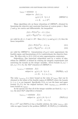
zminlp = minimize f(x)
subject to gj(x) ≤ 0 ∀j ∈ J, (MINLP)
x ∈ X, xI ∈ Z|I|
,
where X is a polyhedral subset of Rn
(e.g. X = {x | x ∈ Rn
+, Ax ≤ b}).
The functions f : X → R and gj : X → R are sufficiently smooth functions.
The algorithms presented here only require continuously differentiable func-
tions, but in general algorithms for solving continuous relaxations converge
much faster if functions are twice-continuously differentiable. The set J is
the index set of nonlinear constraints, I is the index set of discrete variables
and C is the index set of continuous variables, so I ∪ C = {1, . . . , n}.](https://image.slidesharecdn.com/11816511-250518184510-47b062f0/85/Mixed-Integer-Nonlinear-Programming-The-Ima-Volumes-In-Mathematics-And-Its-Applications-2012th-Edition-Leyffer-27-320.jpg)
![4 PIERRE BONAMI, MUSTAFA KILINÇ, AND JEFF LINDEROTH
For convenience, we assume that the set X is bounded; in particular
some finite lower bounds LI and upper bounds UI on the values of the
integer variables are known. In most applications, discrete variables are
restricted to 0-1 values, i.e., xi ∈ {0, 1} ∀i ∈ I. In this survey, we focus on
the case where the functions f and gj are convex. Thus, by relaxing the
integrality constraint on x, a convex program, minimization of a convex
function over a convex set, is formed. We will call such problems convex
MINLPs. From now on, unless stated, we will refer convex MINLPs as
MINLPs.
There are a number of important special cases of MINLP. If f(x) =
xT
Qx + dT
x + h, is a (convex) quadratic function of x, and there are only
linear constraints on the problem (J = ∅), the problem is known as a mixed
integer quadratic program (MIQP). If both f(x) and gj(x) are quadratic
functions of x for each j ∈ J, the problem is known as a mixed integer
quadratically constrained program (MIQCP). Significant work was been
devoted to these important special cases [87, 29, 21].
If the objective function is linear, and all nonlinear constraints have
the form gj(x) = Ax + b2 − cT
x − d, then the problem is a Mixed Integer
Second-Order Cone Program (MISOCP). Through a well-known transfor-
mation, MIQCP can be transformed into a MISOCP. In fact, many different
types of sets defined by nonlinear constraints are representable via second-
order cone inequalities. Discussion of these transformations is out of the
scope of this work, but the interested reader may consult [15]. Relatively
recently, commercial software packages such as CPLEX [66], XPRESS-MP
[47], and Mosek [88] have all been augmented to include specialized al-
gorithms for solving these important special cases of convex MINLPs. In
what follows, we focus on general convex MINLP and software available
for its solution.
2.2. Basic elements of MINLP methods. The basic concept un-
derlying algorithms for solving (MINLP) is to generate and refine bounds
on its optimal solution value. Lower bounds are generated by solving a
relaxation of (MINLP), and upper bounds are provided by the value of
a feasible solution to (MINLP). Algorithms differ in the manner in which
these bounds are generated and the sequence of subproblems that are solved
to generate these bounds. However, algorithms share many basic common
elements, which are described next.
Linearizations: Since the objective function of (MINLP) may be non-
linear, its optimal solution may occur at a point that is interior to the
convex hull of its set of feasible solutions. It is simple to transform the
instance to have a linear objective function by introducing an auxiliary
variable η and moving the original objective function into the constraints.
Specifically, (MINLP) may be equivalently stated as](https://image.slidesharecdn.com/11816511-250518184510-47b062f0/85/Mixed-Integer-Nonlinear-Programming-The-Ima-Volumes-In-Mathematics-And-Its-Applications-2012th-Edition-Leyffer-28-320.jpg)
![6 PIERRE BONAMI, MUSTAFA KILINÇ, AND JEFF LINDEROTH
NLP software typically will deduce infeasibility by solving an associated
feasibility subproblem. One choice of feasibility subproblem employed by
NLP solvers is
zNLPF(x̂I ) = minimize
m
j=1
wjgj(x)+
s.t. x ∈ X, xI = x̂I, (NLPF(x̂I))
where gj(x)+
= max{0, gj(x)} measures the violation of the nonlinear con-
straints and wj ≥ 0. Since when NLP(x̂I) is infeasible NLP solvers will
return the solution to NLPF(x̂I), we will often say, by abuse of terminology,
that NLP(x̂I) is solved and its solution x is optimal or minimally infeasible,
meaning that it is the optimal solution to NLPF(x̂I).
3. Algorithms for convex MINLP. With elements of algorithms
defined, attention can be turned to describing common algorithms for
solving MINLPs. The algorithms share many general characteristics with
the well-known branch-and-bound or branch-and-cut methods for solving
MILPs.
3.1. NLP-Based Branch and Bound. Branch and bound is a
divide-and-conquer method. The dividing (branching) is done by parti-
tioning the set of feasible solutions into smaller and smaller subsets. The
conquering (fathoming) is done by bounding the value of the best feasible
solution in the subset and discarding the subset if its bound indicates that
it cannot contain an optimal solution.
Branch and bound was first applied to MILP by Land and Doig [74].
The method (and its enhancements such as branch and cut) remain the
workhorse for all of the most successful MILP software. Dakin [38] real-
ized that this method does not require linearity of the problem. Gupta
and Ravindran [62] suggested an implementation of the branch-and-bound
method for convex MINLPs and investigated different search strategies.
Other early works related to NLP-Based Branch and Bound (NLP-BB for
short) for convex MINLP include [91], [28], and [78].
In NLP-BB, the lower bounds come from solving the subproblems
(NLPR(lI, uI)). Initially, the bounds (LI, UI) (the lower and upper bounds
on the integer variables in (MINLP)) are used, so the algorithm is initialized
with a continuous relaxation whose solution value provides a lower bound
on zminlp. The variable bounds are successively refined until the subregion
can be fathomed. Continuing in this manner yields a tree L of subproblems.
A node N of the search tree is characterized by the bounds enforced on its
integer variables: N
def
= (lI, uI). Lower and upper bounds on the optimal
solution value zL ≤ zminlp ≤ zU are updated through the course of the
algorithm. Algorithm 1 gives pseudocode for the NLP-BB algorithm for
solving (MINLP).](https://image.slidesharecdn.com/11816511-250518184510-47b062f0/85/Mixed-Integer-Nonlinear-Programming-The-Ima-Volumes-In-Mathematics-And-Its-Applications-2012th-Edition-Leyffer-30-320.jpg)
![ALGORITHMS AND SOFTWARE FOR CONVEX MINLP 7
Algorithm 1 The NLP-Based Branch-and-Bound algorithm
0. Initialize.
L ← {(LI, UI)}. zU = ∞. x∗
← NONE.
1. Terminate?
Is L = ∅? If so, the solution x∗
is optimal.
2. Select.
Choose and delete a problem Ni
= (li
I, ui
I) from L.
3. Evaluate.
Solve NLPR(li
I, ui
I). If the problem is infeasible, go to step 1, else
let znlpr(li
I ,ui
I ) be its optimal objective function value and x̂i
be its
optimal solution.
4. Prune.
If znlpr(li
I ,ui
I ) ≥ zU , go to step 1. If x̂i
is fractional, go to step 5,
else let zU ← znlpr(li
I ,ui
I ), x∗
← x̂i
, and delete from L all problems
with zj
L ≥ zU . Go to step 1.
5. Divide.
Divide the feasible region of Ni
into a number of smaller feasi-
ble subregions, creating nodes Ni1
, Ni2
, . . . , Nik
. For each j =
1, 2, . . . , k, let z
ij
L ← znlpr(li
I ,ui
I ) and add the problem Nij
to L. Go
to 1.
As described in step 4 of Algorithm 1, if NLPR(li
I, ui
I) yields an in-
tegral solution (a solution where all discrete variables take integer values),
then znlpr(li
I ,ui
I ) gives an upper bound for MINLP. Fathoming of nodes oc-
curs when the lower bound for a subregion obtained by solving NLPR(li
I,
ui
I) exceeds the current upper bound zU , when the subproblem is infeasi-
ble, or when the subproblem provides a feasible integral solution. If none
of these conditions is met, the node cannot be pruned and the subregion is
divided to create new nodes. This Divide step of Algorithm 1 may be per-
formed in many ways. In most successful implementations, the subregion
is divided by dichotomy branching. Specifically, the feasible region of Ni
is
divided into subsets by changing bounds on one integer variable based on
the solution x̂i
to NLPR(li
I, ui
I). An index j ∈ I such that x̂j ∈ Z is chosen
and two new children nodes are created by adding the bound xj ≤ x̂j to
one child and xj ≥ x̂j to the other child. The tree search continues until
all nodes are fathomed, at which point x∗
is the optimal solution.
The description makes it clear that there are various choices to be
made during the course of the algorithm. Namely, how do we select which
subproblem to evaluate, and how do we divide the feasible region? A partial
answer to these two questions will be provided in Sections 4.2 and 4.3.
The NLP-Based Branch-and-Bound algorithm is implemented in solvers
MINLP-BB [77], SBB [30], and Bonmin [24].](https://image.slidesharecdn.com/11816511-250518184510-47b062f0/85/Mixed-Integer-Nonlinear-Programming-The-Ima-Volumes-In-Mathematics-And-Its-Applications-2012th-Edition-Leyffer-31-320.jpg)
![8 PIERRE BONAMI, MUSTAFA KILINÇ, AND JEFF LINDEROTH
3.2. Outer Approximation. The Outer Approximation (OA)
method for solving (MINLP) was first proposed by Duran and Grossmann
[43]. The fundamental insight behind the algorithm is that (MINLP)
is equivalent to a Mixed Integer Linear Program (MILP) of finite size.
The MILP is constructed by taking linearizations of the objective and
constraint functions about the solution to the subproblem NLP(x̂I) or
NLPF(x̂I) for various choices of x̂I. Specifically, for each integer assign-
ment x̂I ∈ ProjxI
(X) ∩ Z|I|
(where ProjxI
(X) denotes the projection of X
onto the space of integer constrained variables), let x ∈ arg min NLP(x̂I)
be an optimal solution to the NLP subproblem with integer variables fixed
according to x̂I. If NLP(x̂I) is not feasible, then let x ∈ arg min NLPF(x̂I)
be an optimal solution to its corresponding feasibility problem. Since
ProjxI
(X) is bounded by assumption, there are a finite number of sub-
problems NLP(x̂I). For each of these subproblems, we choose one optimal
solution, and let K be the (finite) set of these optimal solutions. Using
these definitions, an outer-approximating MILP can be specified as
zoa = min η
s.t. η ≥ f(x) + ∇f(x)T
(x − x) x ∈ K, (MILP-OA)
gj(x) + ∇gj(x)T
(x − x) ≤ 0 j ∈ J, x ∈ K,
x ∈ X, xI ∈ ZI
.
The equivalence between (MINLP) and (MILP-OA) is specified in the
following theorem:
Theorem 3.1. [43, 51, 24] If X = ∅, f and g are convex, continuously
differentiable, and a constraint qualification holds for each xk
∈ K then
zminlp = zoa. All optimal solutions of (MINLP) are optimal solutions of
(MILP-OA).
From a practical point of view it is not relevant to try and formulate
explicitly (MILP-OA) to solve (MINLP)—to explicitly build it, one would
have first to enumerate all feasible assignments for the integer variables
in X and solve the corresponding nonlinear programs NLP(x̂I). The OA
method uses an MILP relaxation (MP(K)) of (MINLP) that is built in a
manner similar to (MILP-OA) but where linearizations are only taken at
a subset K of K:
zmp(K) = min η
s.t. η ≥ f(x̄) + ∇f(x̄)T
(x − x̄) x̄ ∈ K, (MP(K))
gj(x̄) + ∇gj(x̄)T
(x − x̄) ≤ 0 j ∈ J, x̄ ∈ K,
x ∈ X, xI ∈ ZI
.
We call this problem the OA-based reduced master problem. The solu-
tion value of the reduced master problem (MP(K)), zmp(K), gives a lower
bound to (MINLP), since K ⊆ K. The OA method proceeds by iteratively](https://image.slidesharecdn.com/11816511-250518184510-47b062f0/85/Mixed-Integer-Nonlinear-Programming-The-Ima-Volumes-In-Mathematics-And-Its-Applications-2012th-Edition-Leyffer-32-320.jpg)
![ALGORITHMS AND SOFTWARE FOR CONVEX MINLP 9
adding points to the set K. Since function linearizations are accumulated
as iterations proceed, the reduced master problem (MP(K)) yields a non-
decreasing sequence of lower bounds.
OA typically starts by solving (NLPR(LI,UI)). Linearizations about
the optimal solution to (NLPR(lI, uI)) are used to construct the first re-
duced master problem (MP(K)). Then, (MP(K)) is solved to optimality to
give an integer solution, x̂. This integer solution is then used to construct
the NLP subproblem (NLP(x̂I)). If (NLP(x̂I)) is feasible, linearizations
about the optimal solution of (NLP(x̂I)) are added to the reduced master
problem. These linearizations eliminate the current solution x̂ from the fea-
sible region of (MP(K)) unless x̂ is optimal for (MINLP). Also, the optimal
solution value zNLP(x̂I ) yields an upper bound to MINLP. If (NLP(x̂I)) is
infeasible, the feasibility subproblem (NLPF(x̂I)) is solved and lineariza-
tions about the optimal solution of (NLPF(x̂I)) are added to the reduced
master problem (MP(K)). The algorithm iterates until the lower and upper
bounds are within a specified tolerance . Algorithm 2 gives pseudocode
for the method. Theorem 3.1 guarantees that this algorithm cannot cycle
and terminates in a finite number of steps.
Note that the reduced master problem need not be solved to optimal-
ity. In fact, given the upper bound UB and a tolerance , it is sufficient
to generate any new (η̂, x̂) that is feasible to (MP(K)), satisfies the in-
tegrality requirements, and for which η ≤ UB − . This can usually be
achieved by setting a cutoff value in the MILP software to enforce the con-
straint η ≤ UB − . If a cutoff value is not used, then the infeasibility of
(MP(K)) implies the infeasibility of (MINLP). If a cutoff value is used, the
OA iterations are terminated (Step 1 of Algorithm 2) when the OA mas-
ter problem has no feasible solution. OA is implemented in the software
packages DICOPT [60] and Bonmin [24].
3.3. Generalized Benders Decomposition. Benders Decomposi-
tion was introduced by Benders [16] for the problems that are linear in the
“easy” variables, and nonlinear in the “complicating“ variables. Geoffrion
[56] introduced the Generalized Benders Decomposition (GBD) method for
MINLP. The GBD method is very similar to the OA method, differing only
in the definition of the MILP master problem. Specifically, instead of us-
ing linearizations for each nonlinear constraint, GBD uses duality theory to
derive one single constraint that combines the linearizations derived from
all the original problem constraints.
In particular, let x be the optimal solution to (NLP(x̂I)) for a given
integer assignment x̂I and μ ≥ 0 be the corresponding optimal Lagrange
multipliers. The following generalized Benders cut is valid for (MINLP)
η ≥f(x) + (∇If(x) + ∇Ig(x)μ)T
(xI − x̂I). (BC(x̂))
Note that xI = x̂I, since the integer variables are fixed. In (BC(x̂)), ∇I
refers to the gradients of functions f (or g) with respect to discrete vari-](https://image.slidesharecdn.com/11816511-250518184510-47b062f0/85/Mixed-Integer-Nonlinear-Programming-The-Ima-Volumes-In-Mathematics-And-Its-Applications-2012th-Edition-Leyffer-33-320.jpg)
![10 PIERRE BONAMI, MUSTAFA KILINÇ, AND JEFF LINDEROTH
Algorithm 2 The Outer Approximation algorithm.
0. Initialize.
zU ← +∞. zL ← −∞. x∗
← NONE. Let x0
be the optimal solution
of (NLPR(LI,UI))
K ←
x0
. Choose a convergence tolerance .
1. Terminate?
Is zU − zL or (MP(K)) infeasible? If so, x∗
is −optimal.
2. Lower Bound
Let zMP(K) be the optimal value of MP(K) and (η̂, x̂) its optimal
solution.
zL ← zMP(K)
3. NLP Solve
Solve (NLP(x̂I)).
Let xi
be the optimal (or minimally infeasible) solution.
4. Upper Bound?
Is xi
feasible for (MINLP) and f(xi
) zU ? If so, x∗
← xi
and
zU ← f(xi
).
5. Refine
K ← K ∪ {xi
} and i ← i + 1.
Go to 1.
ables. The inequality (BC(x̂)) is derived by building a surrogate of the
OA constraints using the multipliers μ and simplifying the result using the
Karush-Kuhn-Tucker conditions satisfied by x (which in particular elimi-
nates the continuous variables from the inequality).
If there is no feasible solution to (NLP(x̂I)), a feasibility cut can be
obtained similarly by using the solution x to (NLPF(x̂I)) and corresponding
multipliers λ ≥ 0:
λ
T
[g(x) + ∇Ig(x)T
(xI − x̂I)] ≤ 0. (FCY(x̂))
In this way, a relaxed master problem similar to (MILP-OA) can be
defined as:
zgbd(KFS,KIS) = min η
s.t. η ≥ f(x) + (∇If(x) + ∇Ig(x)μ)T
(xI − xI) ∀x ∈ KFS,
λ
T
[g(x) + ∇Ig(x)T
(xI − xI)] ≤ 0 ∀x ∈ KIS,
(RM-GBD)
x ∈ X, xI ∈ ZI
,
where KFS is the set of solutions to feasible subproblems (NLP(x̂I)) and
KIS is the set solutions to infeasible subproblems (NLPF(x̂I)). Conver-
gence results for the GBD method are similar to those for OA.](https://image.slidesharecdn.com/11816511-250518184510-47b062f0/85/Mixed-Integer-Nonlinear-Programming-The-Ima-Volumes-In-Mathematics-And-Its-Applications-2012th-Edition-Leyffer-34-320.jpg)
![ALGORITHMS AND SOFTWARE FOR CONVEX MINLP 11
Theorem 3.2. [56] If X = ∅, f and g are convex, and a constraint
qualification holds for each xk
∈ K, then zminlp = zgbd(KFS,KIS). The
algorithm terminates in a finite number of steps.
The inequalities used to create the master problem (RM-GBD) are
aggregations of the inequalities used for (MILP-OA). As such, the lower
bound obtained by solving a reduced version of (RM-GBD) (where only
a subset of the constraints is considered) can be significantly weaker than
for (MP(K)). This may explain why there is no available solver that uses
solely the GBD method for solving convex MINLP. Abhishek, Leyffer and
Linderoth [2] suggest to use the Benders cuts to aggregate inequalities in
an LP/NLP-BB algorithm (see Section 3.5).
3.4. Extended Cutting Plane. Westerlund and Pettersson [111]
proposed the Extended Cutting Plane (ECP) method for convex MINLPs,
which is an extension of Kelley’s cutting plane method [70] for solving
convex NLPs. The ECP method was further extended to handle pseudo-
convex function in the constraints [109] and in the objective [112] in the
α-ECP method. Since this is beyond our definition of (MINLP), we give
only here a description of the ECP method when all functions are convex.
The reader is invited to refer to [110] for an up-to-date description of this
enhanced method. The main feature of the ECP method is that it does not
require the use of an NLP solver. The algorithm is based on the iterative
solution of a reduced master problem (RM-ECP(K)). Linearizations of the
most violated constraint at the optimal solution of (RM-ECP(K)) are added
at every iteration. The MILP reduced master problem (RM-ECP(K)) is
defined as:
zecp(K) = min η
s.t. η ≥ f(x̄) + ∇f(x̄)T
(x − x̄) x̄ ∈ K (RM-ECP(K))
gj(x̄) + ∇gj(x̄)T
(x − x̄) ≤ 0 x̄ ∈ K j ∈ J(x̄)
x ∈ X, xI ∈ ZI
where J(x̄)
def
= {j ∈ arg maxj∈J gj(x̄)} is the index set of most violated
constraints for each solution x̄ ∈ K, the set of solutions to (RM-ECP(K)).
It is also possible to add linearizations of all violated constraints to (RM-
ECP(K)). In that case, J(x̄) = {j | gj(x̄) 0}. Algorithm 3 gives the
pseudocode for the ECP algorithm.
The optimal values zecp(K) of (RM-ECP(K)) generate a non-
decreasing sequence of lower bounds. Finite convergence of the algorithm
is achieved when the maximum constraint violation is smaller than a spec-
ified tolerance . Theorem 3.3 states that the sequence of objective values
obtained from the solutions to (RM-ECP(K)) converge to the optimal so-
lution value.
Theorem 3.3. [111] If X = ∅ is compact and f and g are convex and
continuously differentiable, then zecp(K) converges to zminlp.](https://image.slidesharecdn.com/11816511-250518184510-47b062f0/85/Mixed-Integer-Nonlinear-Programming-The-Ima-Volumes-In-Mathematics-And-Its-Applications-2012th-Edition-Leyffer-35-320.jpg)
![12 PIERRE BONAMI, MUSTAFA KILINÇ, AND JEFF LINDEROTH
The ECP method may require a large number of iterations, since the
linearizations added at Step 3 are not coming from solutions to NLP sub-
problems. Convergence can often be accelerated by solving NLP subprob-
lems (NLP(x̂I)) and adding the corresponding linearizations, as in the OA
method. The Extended Cutting Plane algorithm is implemented in the
α-ECP software [110].
Algorithm 3 The Extended Cutting Plane algorithm
0. Initialize.
Choose convergence tolerance . K ← ∅.
1. Lower Bound
Let (ηi
, xi
) be the optimal solution to (RM-ECP(K)).
2. Terminate?
Is gj(x̄i
) ∀j ∈ J and f(x̄i
) − η̄i
? If so, xi
is optimal with
−feasibility.
3. Refine
K ← K ∪ {xi
}, t ∈ arg maxj gj(x̄i
), and J(x̄i
) = {t}
i ← i + 1. Go to 1.
3.5. LP/NLP-Based Branch-and-Bound. The LP/NLP-Based
Branch-and-Bound algorithm (LP/NLP-BB) was first proposed by Que-
sada and Grossmann [96]. The method is an extension of the OA method
outlined in Section 3.2, but instead of solving a sequence of master prob-
lems (MP(K)), the master problem is dynamically updated in a single
branch-and-bound tree that closely resembles the branch-and-cut method
for MILP.
We denote by LP(K, i
I, ui
I) the LP relaxation of (MP(K)) obtained
by dropping the integrality requirements and setting the lower and upper
bounds on the xI variables to lI and uI respectively. The LP/NLP-BB
method starts by solving the NLP relaxation (NLPR(LI,UI)), and sets up
the reduced master problem (MP(K)). A branch-and-bound enumeration
is then started for (MP(K)) using its LP relaxation. The branch-and-
bound enumeration generates linear programs LP(K, i
I, ui
I) at each node
Ni
= (i
I, ui
I) of the tree. Whenever an integer solution is found at a
node, the standard branch and bound is interrupted and (NLP(x̂i
I)) (and
(NLPF(x̂i
I)) if NLP(x̂i
I) is infeasible) is solved by fixing integer variables
to solution values at that node. The linearizations from the solution of
(NLP(x̂i
I)) are then used to update the reduced master problem (MP(K)).
The branch-and-bound tree is then continued with the updated reduced
master problem. The main advantage of LP/NLP-BB over OA is that
the need of restarting the tree search is avoided and only a single tree is
required. Algorithm 4 gives the pseudo-code for LP/NLP-BB.
Adding linearizations dynamically to the reduced master problem
(MP(K)) is a key feature of LP/NLP-BB. Note, however that the same](https://image.slidesharecdn.com/11816511-250518184510-47b062f0/85/Mixed-Integer-Nonlinear-Programming-The-Ima-Volumes-In-Mathematics-And-Its-Applications-2012th-Edition-Leyffer-36-320.jpg)
![ALGORITHMS AND SOFTWARE FOR CONVEX MINLP 13
idea could potentially be applied to both the GBD and ECP methods. The
LP/NLP-BB method commonly significantly reduces the total number of
nodes to be enumerated when compared to the OA method. However,
the trade-off is that the number of NLP subproblems might increase. As
part of his Ph.D. thesis, Leyffer implemented the LP/NLP-BB method
and reported substantial computational savings [76]. The LP/NLP-Based
Branch-and-Bound algorithm is implemented in solvers Bonmin [24] and
FilMINT [2].
Algorithm 4 The LP/NLP-Based Branch-and-Bound algorithm.
0. Initialize.
L ← {(LI, UI)}. zU ← +∞. x∗
← NONE.
Let x be the optimal solution of (NLPR(lI, uI)).
K ← {x}.
1. Terminate?
Is L = ∅? If so, the solution x∗
is optimal.
2. Select.
Choose and delete a problem Ni
= (li
I, ui
I) from L.
3. Evaluate.
Solve LP(K, li
I, ui
I). If the problem is infeasible, go to step 1, else
let zMPR(K,li
I ,ui
I ) be its optimal objective function value and (η̂i
, x̂i
)
be its optimal solution.
4. Prune.
If zMPR(K,li
I ,ui
I ) ≥ zU , go to step 1.
5. NLP Solve?
Is x̂i
I integer? If so, solve (NLP(x̂i
I)), otherwise go to step 8.
Let xi
be the optimal (or minimally infeasible) solution.
6. Upper bound?
Is xi
feasible for (MINLP) and f(xi
) zU ? If so, x∗
← xi
, zU ←
f(xi
).
7. Refine.
Let K ← K ∪ (xi
). Go to step 3.
8. Divide.
Divide the feasible region of Ni
into a number of smaller feasi-
ble subregions, creating nodes Ni1
, Ni2
, . . . , Nik
. For each j =
1, 2, . . . , k, let z
ij
L ← zMPR(K,li
I ,ui
I ) and add the problem Nij
to L.
Go to step 1.
4. Implementation techniques for convex MINLP. Seasoned al-
gorithmic developers know that proper engineering and implementation can
have a large positive impact on the final performance of software. In this
section, we present techniques that have proven useful in efficiently imple-
menting the convex MINLP algorithms of Section 3.](https://image.slidesharecdn.com/11816511-250518184510-47b062f0/85/Mixed-Integer-Nonlinear-Programming-The-Ima-Volumes-In-Mathematics-And-Its-Applications-2012th-Edition-Leyffer-37-320.jpg)
![14 PIERRE BONAMI, MUSTAFA KILINÇ, AND JEFF LINDEROTH
The algorithms for solving MINLP we presented share a great deal in
common with algorithms for solving MILP. NLP-BB is similar to a branch
and bound for MILP, simply solving a different relaxation at each node.
The LP/NLP-BB algorithm can be viewed as a branch-and-cut algorithm,
similar to those employed to solve MILP, where the refining linearizations
are an additional class of cuts used to approximate the feasible region. An
MILP solver is used as a subproblem solver in the iterative algorithms (OA,
GBD, ECP). In practice, all the methods spend most of their computing
time doing variants of the branch-and-bound algorithm. As such, it stands
to reason that advances in techniques for the implementation of branch
and bound for MILP should be applicable and have a positive impact for
solving MINLP. The reader is referred to the recent survey paper [84] for
details about modern enhancements in MILP software.
First we discuss improvements to the Refine step of LP/NLP-BB,
which may also be applicable to the GBD or ECP methods. We then pro-
ceed to the discussion of the Select and Divide steps which are important
in any branch-and-bound implementation. The section contains an intro-
duction to classes of cutting planes that may be useful for MINLP and
reviews recent developments in heuristics for MINLP.
We note that in the case of iterative methods OA, GBD and ECP,
some of these aspects are automatically taken care of by using a “black-
box” MILP solver to solve (MP(K)) as a component of the algorithm. In
the case of NLP-BB and LP/NLP-BB, one has to more carefully take these
aspects into account, in particular if one wants to be competitive in practice
with methods employing MILP solvers as components.
4.1. Linearization generation. In the OA Algorithm 2, the ECP
Algorithm 3, or the LP/NLP-BB Algorithm 4, a key step is to Refine the
approximation of the nonlinear feasible region by adding linearizations of
the objective and constraint functions (2.1) and (2.2). For convex MINLPs,
linearizations may be generated at any point and still give a valid outer
approximation of the feasible region, so for all of these algorithms, there is
a mechanism for enhancing them by adding many linear inequalities. The
situation is similar to the case of a branch-and-cut solver for MILP, where
cutting planes such as Gomory cuts [59], mixed-integer-rounding cuts [85],
and disjunctive (lift and project) cuts [9] can be added to approximate the
convex hull of integer solutions, but care must be taken in a proper imple-
mentation to not overwhelm the software used for solving the relaxations
by adding too many cuts. Thus, key to an effective refinement strategy in
many algorithms for convex MINLP is a policy for deciding when inequal-
ities should be added and removed from the master problem and at which
points the linearizations should be taken.
Cut Addition: In the branch-and-cut algorithm for solving MILP,
there is a fundamental implementation choice that must be made when
confronted with an infeasible (fractional) solution: should the solution be](https://image.slidesharecdn.com/11816511-250518184510-47b062f0/85/Mixed-Integer-Nonlinear-Programming-The-Ima-Volumes-In-Mathematics-And-Its-Applications-2012th-Edition-Leyffer-38-320.jpg)
![ALGORITHMS AND SOFTWARE FOR CONVEX MINLP 15
eliminated by cutting or branching? Based on standard ideas employed
for answering this question in the context of MILP, we offer three rules-of-
thumb that are likely to be effective in the context of linearization-based
algorithms for solving MINLP. First, linearizations should be generated
early in the procedure, especially at the very top of the branch-and-bound
tree. Second, the incremental effectiveness of adding additional lineariza-
tions should be measured in terms of the improvement in the lower bound
obtained. When the rate of lower bound change becomes too low, the
refinement process should be stopped and the feasible region divided in-
stead. Finally, care must be taken to not overwhelm the solver used for the
relaxations of the master problem with too many linearizations.
Cut Removal: One simple strategy for limiting the number of linear
inequalities in the continuous relaxation of the master problem (MP(K)) is
to only add inequalities that are violated by the current solution to the lin-
ear program. Another simple strategy for controlling the size of (MP(K))
is to remove inactive constraints from the formulation. One technique is
to monitor the dual variable for the row associated with the linearization.
If the value of the dual variable is zero, implying that removal of the in-
equality would not change the optimal solution value, for many consecutive
solutions, then the linearization is a good candidate to be removed from
the master problem. To avoid cycling, the removed cuts are usually stored
in a pool. Whenever a cut of the pool is found to be violated by the current
solution it is put back into the formulation.
Linearization Point Selection. A fundamental question in any
linearization-based algorithm (like OA, ECP, or LP/NLP-BB) is at which
points should the linearizations be taken. Each algorithm specifies a mini-
mal set of points at which linearizations must be taken in order to ensure
convergence to the optimal solution. However, the algorithm performance
may be improved by additional linearizations. Abhishek, Leyffer, and Lin-
deroth [2] offer three suggestions for choosing points about which to take
linearizations.
The first method simply linearizes the functions f and g about the
fractional point x̂ obtained as a solution to an LP relaxation of the master
problem. This method does not require the solution of an additional (non-
linear) subproblem, merely the evaluation of the gradients of objective and
constraint functions at the (already specified) point. (The reader will note
the similarity to the ECP method).
A second alternative is to obtain linearizations about a point that is
feasible with respect to the nonlinear constraints. Specifically, given a (pos-
sibly fractional) solution x̂, the nonlinear program (NLP(x̂I)) is solved to
obtain the point about which to linearize. This method has the advan-
tage of generating linearization about points that are closer to the feasible
region than the previous method, at the expense of solving the nonlinear
program (NLP(x̂I)).](https://image.slidesharecdn.com/11816511-250518184510-47b062f0/85/Mixed-Integer-Nonlinear-Programming-The-Ima-Volumes-In-Mathematics-And-Its-Applications-2012th-Edition-Leyffer-39-320.jpg)
![16 PIERRE BONAMI, MUSTAFA KILINÇ, AND JEFF LINDEROTH
In the third point-selection method, no variables are fixed (save those
that are fixed by the nodal subproblem), and the NLP relaxation (NLPR(lI,
uI)) is solved to obtain a point about which to generate linearizations.
These linearizations are likely to improve the lower bound by the largest
amount when added to the master problem since the bound obtained after
adding the inequalities is equal to zNLPR(li,ui), but it can be time-consuming
to compute the linearizations.
These three classes of linearizations span the trade-off spectrum of
time required to generate the linearization versus the quality/strength of
the resulting linearization. There are obviously additional methodologies
that may be employed, giving the algorithm developer significant freedom
to engineer linearization-based methods.
4.2. Branching rules. We now turn to the discussion of how to split
a subproblem in the Divide step of the algorithms. As explained in Section
2.1, we consider here only branching by dichotomy on the variables. Sup-
pose that we are at node Ni
of the branch-and-bound tree with current
solution x̂i
. The goal is to select an integer-constrained variable xj ∈ I
that is not currently integer feasible (x̂i
j ∈ Z) to create two subproblems
by imposing the constraint xj ≤ x̂i
j (branching down) and xj ≥ x̂i
j
(branching up) respectively. Ideally, one would want to select the vari-
able that leads to the smallest enumeration tree. This of course cannot be
performed exactly, since the variable which leads to the smallest subtree
cannot be know a priori.
A common heuristic reasoning to choose the branching variable is to
try to estimate how much one can improve the lower bound by branching
on each variable. Because a node of the branch-and-bound tree is fathomed
whenever the lower bound for the node is above the current upper bound,
one should want to increase the lower bound as much as possible. Suppose
that, for each variable xj, we have estimates Di
j− and Di
j+ on the increase
in the lower bound value obtained by branching respectively down and up.
A reasonable choice would be to select the variable for which both Di
j− and
Di
j+ are large. Usually, Di
j− and Di
j+ are combined in order to compute
a score for each variable and the variable of highest score is selected. A
common formula for computing this score is:
μ min(Di
j−, Di
j+) + (1 − μ) max(Di
j−, Di
j+)
(where μ ∈ [0, 1] is a prescribed parameter typipcally larger than 1
2 ).
As for the evaluation or estimation of Di
j− and Di
j+, two main methods
have been proposed: pseudo-costs [17] and strong-branching [66, 6]. Next,
we will present these two methods and how they can be combined.
4.2.1. Strong-branching. Strong-branching consists in computing
the values Di
j− and Di
j+ by performing the branching on variable xj and
solving the two associated sub-problems. For each variable xj currently](https://image.slidesharecdn.com/11816511-250518184510-47b062f0/85/Mixed-Integer-Nonlinear-Programming-The-Ima-Volumes-In-Mathematics-And-Its-Applications-2012th-Edition-Leyffer-40-320.jpg)
![ALGORITHMS AND SOFTWARE FOR CONVEX MINLP 17
fractional in x̂i
j, we solve the two subproblems Ni
j− and Ni
j+ obtained by
branching down and up, respectively, on variable j. Because Ni
j− and/or
Ni
j+ may be proven infeasible, depending on their status, different decision
may be taken.
• If both sub-problems are infeasible: the node Ni
is infeasible and
is fathomed.
• If one of the subproblems is infeasible: the bound on variable xj can
be strengthened. Usually after the bound is modified, the node is
reprocessed from the beginning (going back to the Evaluate step).
• If both subproblems are feasible, their values are used to compute
Di
j− and Di
j+.
Strong-branching can very significantly reduce the number of nodes
in a branch-and-bound tree, but is often slow overall due to the added
computing cost of solving two subproblems for each fractional variable.
To reduce the computational cost of strong-branching, it is often efficient
to solve the subproblems only approximately. If the relaxation at hand
is an LP (for instance in LP/NLP-BB) it can be done by limiting the
number of dual simplex iterations when solving the subproblems. If the
relaxation at hand is an NLP, it can be done by solving an approximation
of the problem to solve. Two possible relaxations that have been recently
suggested [23, 106, 80] are the LP relaxation obtained by constructing an
Outer Approximation or the Quadratic Programming approximation given
by the last Quadratic Programming sub-problem in a Sequential Quadratic
Programming (SQP) solver for nonlinear programming (for background on
SQP solvers see [94]).
4.2.2. Pseudo-costs. The pseudo-costs method consists in keeping
the history of the effect of branching on each variable and utilizing this
historical information to select good branching variables. For each variable
xj, we keep track of the number of times the variable has been branched on
(τj) and the total per-unit degradation of the objective value by branching
down and up, respectively, Pj− and Pj+. Each time variable j is branched
on, Pj− and Pj+ are updated by taking into account the change of bound
at that node:
Pj− =
zi−
L − zi
L
fi
j
+ Pj−, and Pj+ =
zi+
L − zi
L
1 − fi
j
+ Pj+,
where xj is the branching variable, Ni
− and Ni
+ denote the nodes from
the down and up branch, zi
L (resp. zi−
L and zi+
L ) denote the lower bounds
computed at node Ni
(resp. Ni
− and Ni
+), and fi
j = x̂i
j − x̂i
j denotes
the fractional part of x̂i
j. Whenever a branching decision has to be made,
estimates of Di
j−, Di
j+ are computed by multiplying the average of observed
degradations with the current fractionality:
Di
j− = fi
j
Pj−
τj
, and Di
j+ = (1 − fi
j )
Pj+
τj
.](https://image.slidesharecdn.com/11816511-250518184510-47b062f0/85/Mixed-Integer-Nonlinear-Programming-The-Ima-Volumes-In-Mathematics-And-Its-Applications-2012th-Edition-Leyffer-41-320.jpg)
![18 PIERRE BONAMI, MUSTAFA KILINÇ, AND JEFF LINDEROTH
Note that contrary to strong-branching, pseudo-costs require very little
computation since the two values Pi
j− and Pi
j+ are only updated once
the values zi−
L and zi+
L have been computed (by the normal process of
branch and bound). Thus pseudo-costs have a negligible computational
cost. Furthermore, statistical experiments have shown that pseudo-costs
often provide reasonable estimates of the objective degradations caused by
branching [83] when solving MILPs.
Two difficulties arise with pseudo-costs. The first one, is how to update
the historical data when a node is infeasible. This matter is not settled.
Typically, the pseudo-costs update is simply ignored if a node is infeasible.
The second question is how the estimates should be initialized. For
this, it seems that the agreed upon state-of-the art is to combine pseudo-
costs with strong-branching, a method that may address each of the two
methods’ drawbacks— strong-branching is too slow to be performed at
every node of the tree, and pseudo-costs need to be initialized. The idea
is to use strong-branching at the beginning of the tree search, and once all
pseudo-costs have been initialized, to revert to using pseudo-costs. Several
variants of this scheme have been proposed. A popular one is reliability
branching [4]. This rule depends on a reliability parameter κ (usually a
natural number between 1 and 8), pseudo-costs are trusted for a particular
variable only after strong-branching has been performed κ times on this
variable.
Finally, we note that while we have restricted ourselves in this dis-
cussion to dichotomy branching, one can branch in many different ways.
Most state-of-the-art solvers allow branching on SOS constraints [14]. More
generally, one could branch on split disjunctions of the form (πT
xI ≤
π0) ∨ (πT
xI ≥ π0 + 1) (where (π, π0) ∈ Zn+1
). Although promising results
have been obtained in the context of MILP [69, 37], as far as we know, these
methods have not been used yet in the context of MINLPs. Finally, meth-
ods have been proposed to branch efficiently in the presence of symmetries
[86, 95]. Again, although they would certainly be useful, these methods
have not yet been adapted into software for solving MINLPs, though some
preliminary work is being done in this direction [81].
4.3. Node selection rules. The other important strategic decision
left unspecified in Algorithms 1 and 4 is which node to choose in the Select
step. Here two goals needs to be considered: decreasing the global upper
bound zU
by finding good feasible solutions, and proving the optimality of
the current incumbent x∗
by increasing the lower bound as fast as possible.
Two classical node selection strategies are depth-first-search and best-first
(or best-bound). As its name suggest, depth first search selects at each
iteration the deepest node of the enumeration tree (or the last node put
in L). Best-first follows an opposite strategy of picking the open node Ni
with the smallest zi
L (the best lower bound).](https://image.slidesharecdn.com/11816511-250518184510-47b062f0/85/Mixed-Integer-Nonlinear-Programming-The-Ima-Volumes-In-Mathematics-And-Its-Applications-2012th-Edition-Leyffer-42-320.jpg)
![ALGORITHMS AND SOFTWARE FOR CONVEX MINLP 19
Both these strategies have their inherent strengths and weaknesses.
Depth-first has the advantage of keeping the size of the list of open-nodes
as small as possible. Furthermore, the changes from one subproblem to
the next are minimal, which can be very advantageous for subproblem
solvers that can effective exploit “warm-start” information. Also, depth-
first search is usually able to find feasible solutions early in the tree search.
On the other hand, depth-first can exhibit extremely poor performance
if no good upper bound is known or found: it may explore many nodes
with lower bound higher than the actual optimal solution. Best-bound has
the opposite strengths and weaknesses. Its strength is that, for a fixed
branching, it minimizes the number of nodes explored (because all nodes
explored by it would be explored independently of the upper bound). Its
weaknesses are that it may require significant memory to store the list L
of active nodes, and that it usually does not find integer feasible solutions
before the end of the search. This last property may not be a shortcoming
if the goal is to prove optimality but, as many applications are too large
to be solved to optimality, it is particularly undesirable that a solver based
only on best-first aborts after several hours of computing time without
producing one feasible solution.
It should seem natural that good strategies are trying to combine both
best-first and depth first. Two main approaches are two-phase methods
[54, 13, 44, 83] and diving methods [83, 22].
Two-phase methods start by doing depth-first to find one (or a small
number of) feasible solution. The algorithm then switches to best-first in
order to try to prove optimality (if the tree grows very large, the method
may switch back to depth-first to try to keep the size of the list of active
nodes under control).
Diving methods are also two-phase methods in a sense. The first phase
called diving does depth-first search until a leaf of the tree (either an integer
feasible or an infeasible one) is found. When a leaf is found, the next node
is selected by backtracking in the tree for example to the node with best
lower bound, and another diving is performed from that node. The search
continues by iterating diving and backtracking.
Many variants of these two methods have been proposed in context
of solving MILP. Sometimes, they are combined with estimations of the
quality of integer feasible solutions that may be found in a subtree com-
puted using pseudo-costs (see for example [83]). Computationally, it is not
clear which of these variants performs better. A variant of diving called
probed diving that performs reasonably well was described by Bixby and
Rothberg [22]. Instead of conducting a pure depth-first search in the diving
phase, the probed diving method explores both children of the last node,
continuing the dive from the best one of the two (in terms of bounds).
4.4. Cutting planes. Adding inequalities to the formulation so that
its relaxation will more closely approximate the convex hull of integer fea-](https://image.slidesharecdn.com/11816511-250518184510-47b062f0/85/Mixed-Integer-Nonlinear-Programming-The-Ima-Volumes-In-Mathematics-And-Its-Applications-2012th-Edition-Leyffer-43-320.jpg)
![20 PIERRE BONAMI, MUSTAFA KILINÇ, AND JEFF LINDEROTH
sible solutions was a major reason for the vast improvement in MILP so-
lution technology [22]. To our knowledge, very few, if any MINLP solvers
add inequalities that are specific to the nonlinear structure of the problem.
Nevertheless, a number of cutting plane techniques that could be imple-
mented have been developed in the literature. Here we outline a few of
these techniques. Most of them have been adapted from known methods in
the MILP case. We refer the reader to [36] for a recent survey on cutting
planes for MILP.
4.4.1. Gomory cuts. The earliest cutting planes for Mixed Integer
Linear Programs were Gomory Cuts [58, 59]. For simplicity of exposition,
we assume a pure Integer Linear Program (ILP): I = {1, . . . , n}, with
linear constraints given in matrix form as Ax ≤ b and x ≥ 0. The idea
underlying the inequalities is to choose a set of non-negative multipliers
u ∈ Rm
+ and form the surrogate constraint uT
Ax ≤ uT
b. Since x ≥ 0, the
inequality
j∈N uT
ajxj ≤ uT
b is valid, and since uT
ajxj is an integer,
the right-hand side may also be rounded down to form the Gomory cut
j∈N uT
ajxj ≤ uT
b. This simple procedure suffices to generate all
valid inequalities for an ILP [35]. Gomory cuts can be generalized to Mixed
Integer Gomory (MIG) cuts which are valid for MILPs. After a period of
not being used in practice to solve MILPs, Gomory cuts made a resurgence
following the work of Balas et al. [10], which demonstrated that when used
in combination with branch and bound, MIG cuts were quite effective in
practice.
For MINLP, Cezik and Iyengar [34] demonstrate that if the nonlinear
constraint set gj(x) ≤ 0 ∀j ∈ J can be described using conic constraints
Tx K b , then the Gomory procedure is still applicable. Here K, is a
homogeneous, self-dual, proper, convex cone, and the notation x K y de-
notes that (x − y) ∈ K. Each cone K has a dual cone K∗
with the property
that K∗ def
= {u | uT
z ≥ 0 ∀z ∈ K} . The extension of the Gomory proce-
dure to the case of conic integer programming is clear from the following
equivalence:
Ax K b ⇔ uT
Ax ≥ uT
b ∀u K∗ 0.
Specifically, elements from the dual cone u ∈ K∗
can be used to perform
the aggregation, and the regular Gomory procedure applied. To the au-
thors’ knowledge, no current MINLP software employs conic Gomory cuts.
However, most solvers generate Gomory cuts from the existing linear in-
equalities in the model. Further, as pointed out by Akrotirianakis, Maros,
and Rustem [5], Gomory cuts may be generated from the linearizations
(2.1) and (2.2) used in the OA, ECP, or LP/NLP-BB methods. Most
linearization-based software will by default generate Gomory cuts on these
linearizations.
4.4.2. Mixed integer rounding. Consider the simple two-variable
set X = {(x1, x2) ∈ Z × R+ | x1 ≤ b + x2}. It is easy to see that the](https://image.slidesharecdn.com/11816511-250518184510-47b062f0/85/Mixed-Integer-Nonlinear-Programming-The-Ima-Volumes-In-Mathematics-And-Its-Applications-2012th-Edition-Leyffer-44-320.jpg)
![ALGORITHMS AND SOFTWARE FOR CONVEX MINLP 21
mixed integer rounding inequality x1 ≤ b + 1
1−f x2, where f = b − b
represents the fractional part of b, is a valid inequality for X. Studying the
convex hull of this simple set and some related counterparts have generated
a rich classes of inequalities that may significantly improve the ability to
solve MILPs [85]. Key to generating useful inequalities for computation
is to combine rows of the problem in a clever manner and to use variable
substitution techniques.
Atamtürk and Narayan [7] have extended the concept of mixed integer
rounding to the case of Mixed Integer Second-Order Cone Programming
(MISOCP). For the conic mixed integer set
T =
(x1, x2, x3) ∈ Z × R2
|
(x1 − b)2 + x2
2 ≤ x3
the following simple conic mixed integer rounding inequality
[(1 − 2f)(x1 − b) + f]2 + x2
2 ≤ x3
helps to describe the convex hull of T. They go on to show that employing
these inequalities in a cut-and-branch procedure for solving MISOCPs is
significantly beneficial. To the authors’ knowledge, no available software
employs this technology, so this may be a fruitful line of computational
research.
4.4.3. Disjunctive inequalities. Stubbs and Mehrotra [101], build-
ing on the earlier seminal work of Balas [8] on disjunctive programming
and its application to MILP (via lift and project cuts) of Balas, Ceria and
Cornuéjols [9], derive a lift and project cutting plane framework for convex
(0-1) MINLPs. Consider the feasible region of the continuous relaxation
of (MINLP-1) R = {(x, η) | f(x) ≤ η, gj(x) ≤ 0 ∀j ∈ J, x ∈ X}. The
procedure begins by choosing a (branching) dichotomy xi = 0 ∨ xi = 1
for some i ∈ I. The convex hull of the union of the two (convex) sets
R−
i
def
= {(x, η) ∈ R | xi = 0}, R+
i = {(x, η) ∈ R | xi = 1} can be repre-
sented in a space of dimension 3n + 5 as
Mi(R) =
⎧
⎪
⎪
⎨
⎪
⎪
⎩
(x, η, x−
, η−
,
x+
, η+
, λ−
, λ+
)
x = λ−
x−
+ λ+
x+
,
η = λ−
η−
+ λ+
η+
,
λ−
+ λ+
= 1, λ−
≥ 0, λ+
≥ 0
(x−
, η−
) ∈ R−
i , (x+
, η+
) ∈ R+
i
⎫
⎪
⎪
⎬
⎪
⎪
⎭
.
One possible complication with the convex hull description Mi(R) is
caused by the nonlinear, nonconvex relationships x = λ−
x−
+ λ+
x+
and
η = λ−
η−
+ λ+
η+
. However, this description can be transformed to an
equivalent description M̃i(R) with only convex functional relationships be-
tween variables using the perspective function [101, 65].](https://image.slidesharecdn.com/11816511-250518184510-47b062f0/85/Mixed-Integer-Nonlinear-Programming-The-Ima-Volumes-In-Mathematics-And-Its-Applications-2012th-Edition-Leyffer-45-320.jpg)
![22 PIERRE BONAMI, MUSTAFA KILINÇ, AND JEFF LINDEROTH
Given some solution (x̄, η̄) /
∈ conv(R−
i ∪ R+
i ), the lift and project
procedure operates by solving a convex separation problem
min
(x,η,x̃−,η̃−,x̃+,η̃+,λ−,λ+)∈M̃i(R)
d(x, η) (4.1)
(where d(x, η) is the distance to the point (x̄, η̄) in any norm). The lift-
and-project inequality
ξT
x (x − x̄) + ξT
η (η − η̄) ≥ 0 (4.2)
separates (x̄, η̄) from conv(R−
i ∪R+
i ), where ξ is a subgradient of d(x, η) at
the optimal solution of (4.1).
An implementation and evaluation of some of these ideas in the context
of MISOCP has been done by Drewes [41]. Cezik and Iyengar [34] had
also stated that the application of disjunctive cuts to conic-IP should be
possible.
A limitation of disjunctive inequalities is that in order to generate a
valid cut, one must solve an auxiliary (separation) problem that is three
times the size of the original relaxation. In the case of MILP, clever intu-
ition of Balas and Perregaard [11] allow to solve this separation problem
while staying in the original space. No such extension is known in the case
of MINLP. Zhu and Kuno [114] have suggested to replace the true nonlin-
ear convex hull by a linear approximation taken about the solution to a
linearized master problem like MP(K).
Kılınç et al. [71] have recently made the observation that a weaker
form of the lift and project inequality (4.2) can be obtained from branching
dichotomy information. Specifically, given values η̂−
i = min{η|(x, η) ∈ R−
i }
and η̂+
i min{η|(x, η) ∈ R+
i }, the strong-branching cut
η ≥ η̂−
i + (η̂+
i − η̂−
i )xi
is valid for MINLP, and is a special case of (4.2). Note that if strong-
branching is used to determine the branching variable, then the values η̂−
i
and η̂+
i are produced as a byproduct.
4.5. Heuristics. Here we discuss heuristic methods that are aimed at
finding integer feasible solutions to MINLP with no guarantee of optimality
or success. Heuristics are usually fast algorithms. In a branch-and-bound
algorithm they are typically run right after the Evaluate step. Depending
on the actual running time of the heuristic, it may be called at every node,
every nth
node, or only at the root node. In linearization-based methods
like OA, GBD, ECP, or LP/NLP-BB, heuristics may be run in the Upper
Bound and Refine step, especially in the case when NLP(x̂I) is infeasible.
Heuristics are very important because by improving the upper bound zU ,
they help in the Prune step of the branch-and-bound algorithm or in the
convergence criterion of the other algorithms. From a practical point of](https://image.slidesharecdn.com/11816511-250518184510-47b062f0/85/Mixed-Integer-Nonlinear-Programming-The-Ima-Volumes-In-Mathematics-And-Its-Applications-2012th-Edition-Leyffer-46-320.jpg)
![ALGORITHMS AND SOFTWARE FOR CONVEX MINLP 23
view, heuristics are extremely important when the algorithm cannot be
carried out to completion, so that a feasible solution may be returned to
the user.
Many heuristic methods have been devised for MILP, we refer the
reader to [19] for a recent and fairly complete review. For convex MINLP,
two heuristic principles that have been used are diving heuristics and the
feasibility pump.
We note that several other heuristic principles could be used such as
RINS [39] or Local Branching [49] but as far as we know, these have not
been applied yet to (convex) MINLPs and we will not cover them here.
4.5.1. Diving heuristics. Diving heuristics are very related to the
diving strategies for node selection presented in Section 4.3. The basic
principle is to simulate a dive from the current node to a leaf of the tree
by fixing variables (either one at a time or several variables at a time).
The most basic scheme is, after the NLP relaxation has been solved, to
fix the variable which is the least integer infeasible in the current solution
to the closest integer and resolve. This process is iterated until either the
current solution is integer feasible or the NLP relaxation becomes infeasible.
Many variants of this scheme have been proposed for MILP (see [19] for
a good review). These differ mainly in the the number of variables fixed,
the way to select variables to fix, and in the possibility of doing a certain
amount of backtracking (unfixing previously fixed variables). The main
difficulty when one tries to adapt these scheme to MINLP is that instead
of having to resolve an LP with a modified bound at each iteration (an
operation which is typically done extremely efficiently by state-of-the-art
LP solvers) one has to solve an NLP (where warm-starting methods are
usually much less efficient).
Bonami and Gonçalves [26] have adapted the basic scheme to MINLPs
in two different manners. First in a straightforward way, but trying to limit
the number of NLPs solved by fixing many variables at each iteration and
backtracking if the fixings induce infeasibility. The second adaptation tries
to reduce the problem to a MILP by fixing all the variables that appear in
a nonlinear term in the objective or the constraints. This MILP problem
may be given to a MILP solver in order to find a feasible solution. A similar
MINLP heuristic idea of fixing variables to create MILPs can be found in
the work [20].
4.5.2. Feasibility pumps. The feasibility pump is another heuristic
principle for quickly finding feasible solutions. It was initially proposed by
Fischetti, Glover and Lodi [48] for MILP, and can be extended to convex
MINLP in several manners.
First we present the feasibility pump in its most trivial extension to
MINLP. The basic principle of the Feasibility Pump consists of generating
a sequence of points x0
, . . . , xk
that satisfy the constraints of the contin-
uous relaxation NLPR(LI,UI). Associated with the sequence x0
, . . . , xk](https://image.slidesharecdn.com/11816511-250518184510-47b062f0/85/Mixed-Integer-Nonlinear-Programming-The-Ima-Volumes-In-Mathematics-And-Its-Applications-2012th-Edition-Leyffer-47-320.jpg)
![24 PIERRE BONAMI, MUSTAFA KILINÇ, AND JEFF LINDEROTH
of integer infeasible points is a sequence x̂1
, . . . , x̂k+1
of points that are
integer feasible but do not necessarily satisfy the other constraints of the
problem. Specifically, x0
is the optimal solution of NLPR(LI,UI). Each
x̂i+1
is obtained by rounding xi
j to the nearest integer for each j ∈ I and
keeping the other components equal to xi
j. The sequence xi
is generated
by solving a nonlinear program whose objective function is to minimize the
distance of x to x̂i
on the integer variables according to the 1-norm:
zFP-NLP(x̂I ) = minimize
k∈I
|xk − x̂i
k|
subject to gj(x) ≤ 0 ∀j ∈ J, (FP-NLP(x̂I))
x ∈ X; LI ≤ x̂I ≤ UI.
The two sequences have the property that at each iteration the distance
between xi
and x̂i+1
is non-increasing. The procedure stops whenever an
integer feasible solution is found (or x̂k
= xk
). This basic procedure may
cycle or stall without finding an integer feasible solution and randomization
has been suggested to restart the procedure [48]. Several variants of this
basic procedure have been proposed in the context of MILP [18, 3, 50].
The authors of [1, 26] have shown that the basic principle of the Feasibility
Pump can also find good solutions in short computing time also in the
context of MINLP.
Another variant of the Feasibility Pump for convex MINLPs was pro-
posed by Bonami et al. [25]. Like in the basic FP scheme two sequences
are constructed with the same properties: x0
, . . . , xk
are points in X that
satisfy g(xi
) ≤ 0 but not xi
I ∈ Z|I|
and x̂1
, . . . , x̂k+1
are points that do
not necessarily satisfy g(x̂i
) ≤ 0 but satisfy x̂i
I ∈ Z|I|
. The sequence xi
is
generated in the same way as before but the sequence x̂i
is now generated
by solving MILPs. The MILP to solve for finding x̂i+1
is constructed by
building an outer approximation of the constraints of the problem with
linearizations taken in all the points of the sequence x0
, . . . , xi
. Then, x̂i+1
is found as the point in the current outer approximation of the constraints
that is closest to xi
in 1-norm in the space of integer constrained variables:
zFP-Mi = minimize
i∈I
|xj − xi
j|
s.t. g(xl
) + ∇g(xl
)T
(x − xl
) ≤ 0 l = 1, . . . , i, (M-FPi
)
x ∈ X, xI ∈ ZI
.
Unlike the procedure of Fischetti, Glover and Lodi, the Feasibility
Pump for MINLP cannot cycle and it is therefore an exact algorithm:
either it finds a feasible solution or it proves that none exists. This variant
of the FP principle can also be seen as a variant of the Outer Approximation
decomposition scheme presented in Section 3.2. In [25], it was also proposed](https://image.slidesharecdn.com/11816511-250518184510-47b062f0/85/Mixed-Integer-Nonlinear-Programming-The-Ima-Volumes-In-Mathematics-And-Its-Applications-2012th-Edition-Leyffer-48-320.jpg)
![ALGORITHMS AND SOFTWARE FOR CONVEX MINLP 25
to iterate the FP scheme by integrating the linearization of the objective
function in the constraint system of (M-FPi
) turning the feasibility pump
into an exact iterative algorithm which finds solutions of increasingly better
cost until eventually proving optimality. Abhishek et al. [1] have also
proposed to integrate this Feasibility Pump into a single tree search (in the
same way as Outer Approximation decomposition can be integrated in a
single tree search when doing the LP/NLP-BB).
5. Software. There are many modern software packages implement-
ing the algorithms of Section 3 that employ the modern enhancements
described in Section 5. In this section, we describe the features of six dif-
ferent packages. The focus is on solvers for general convex MINLPs, not
only special cases such as MIQP, MIQCP, or MISOCP. All of these pack-
ages may be freely used via a web interface on NEOS (http://www-neos.
mcs.anl.gov).
5.1. α-ECP. α-ECP [110] is a solver based on the ECP method de-
scribed in Section 3.4. Problems to be solved may be specified in a text-
based format, as user-supplied subroutines, or via the GAMS algebraic
modeling language. The software is designed to solve convex MINLP, but
problems with a pseudo-convex objective function and pseudo-convex con-
straints can also be solved to global optimality with α-ECP. A significant
feature of the software is that no nonlinear subproblems are required to
be solved. (Though recent versions of the code have included an option to
occasionally solve NLP subproblems, which may improve performance, es-
pecially on pseudo-convex instances.) Recent versions of the software also
include enhancements so that each MILP subproblem need not be solved to
global optimality. α-ECP requires a (commercial) MILP software to solve
the reduced master problem (RM-ECP(K)), and CPLEX, XPRESS-MP,
or Mosek may be used for this purpose.
In the computational experiment of Section 6, α-ECP (v1.75.03) is
used with CPLEX (v12.1) as MILP solver, CONOPT (v3.24T) as NLP
solver and α-ECP is run via GAMS. Since all instances are convex, setting
the ECPstrategy option to 1 instructed α-ECP to not perform algorithmic
steps relating to the solution of pseudo-convex instances.
5.2. Bonmin. Bonmin is an open-source MINLP solver and frame-
work with implementations of algorithms NLP-BB, OA, and two different
LP/NLP-BB algorithms with different default parameters. Source code and
binaries of Bonmin are available from COIN-OR (http://www.coin-or.
org). Bonmin may be called as a solver from both the AMPL and GAMS
modeling languages.
Bonmin interacts with the COIN-OR software Cbc to manage the
branch-and-bound trees of its various algorithms. To solve NLP subprob-
lems, Bonmin may be instrumented to use either Ipopt [107] or FilterSQP
[52]. Bonmin uses the COIN-OR software Clp to solve linear programs,](https://image.slidesharecdn.com/11816511-250518184510-47b062f0/85/Mixed-Integer-Nonlinear-Programming-The-Ima-Volumes-In-Mathematics-And-Its-Applications-2012th-Edition-Leyffer-49-320.jpg)
![26 PIERRE BONAMI, MUSTAFA KILINÇ, AND JEFF LINDEROTH
and may use Cbc or Cplex to solve MILP subproblems arising in its vari-
ous algorithms.
The Bonmin NLP-BB algorithm features a range of different heuris-
tics, advanced branching techniques such as strong-branching or pseudo-
costs branching, and five different choices for node selection strategy. The
Bonmin LP/NLP-BB methods use row management, cutting planes, and
branching strategies from Cbc. A distinguishing feature of Bonmin is that
one may instruct Bonmin to use a (time-limited) OA or feasibility pump
heuristic at the beginning of the optimization.
In the computational experiments, Bonmin (v1.1) is used with Cbc
(v2.3) as the MILP solver, Ipopt (v2.7) as NLP solver, and Clp (v1.10)
is used as LP solver. For Bonmin, the algorithms, NLP-BB (denoted
as B-BB) and LP/NLP-BB (denoted as B-Hyb) are tested. The default
search strategies of dynamic node selection (mixture of depth-first-search
and best-bound) and strong-branching were employed.
5.3. DICOPT. DICOPT is a software implementation of the OA
method described in Section 3.2. DICOPT may be used as a solver from the
GAMS modeling language. Although OA has been designed to solve convex
MINLP, DICOPT may often be used successfully as a heuristic approach
for nonconvex MINLP, as it contains features such as equality relaxation
[72] and augmented penalty methods [105] for dealing with nonconvexities.
DICOPT requires solvers for both NLP subproblems and MILP subprob-
lems, and it uses available software as a “black-box” in each case. For NLP
subproblems, possible NLP solvers include CONOPT [42], MINOS [89]
and SNOPT [57]. For MILP subproblems, possible MILP solvers include
CPLEX [66] and XPRESS [47]. DICOPT contains a number of heuristic
(inexact) stopping rules for the OA method that may be especially effective
for nonconvex instances.
In our computational experiment, the DICOPT that comes with
GAMS v23.2.1 is used with CONOPT (v3.24T) as the NLP solver and
Cplex (v12.1) as the MILP solver. In order to ensure that instances are
solved to provable optimality, the GAMS/DICOPT option stop was set to
value 1.
5.4. FilMINT. FilMINT [2] is a non-commercial solver for convex
MINLPs based on the LP/NLP-BB algorithm. FilMINT may be used
through the AMPL language.
FilMINT uses MINTO [93] a branch-and-cut framework for MILP to
solve the reduced master problem (MP(K)) and filterSQP [52] to solve
nonlinear subproblems. FilMINT uses the COIN-OR LP solver Clp or
CPLEX to solve linear programs.
FilMINT by default employs nearly all of MINTO’s enhanced MILP
features, such as cutting planes, primal heuristics, row management, and
enhanced branching and node selection rules. By default, pseudo-costs
branching is used as branching strategy and best estimate is used as node](https://image.slidesharecdn.com/11816511-250518184510-47b062f0/85/Mixed-Integer-Nonlinear-Programming-The-Ima-Volumes-In-Mathematics-And-Its-Applications-2012th-Edition-Leyffer-50-320.jpg)
![ALGORITHMS AND SOFTWARE FOR CONVEX MINLP 27
selection strategy. An NLP-based Feasibility Pump can be run at the be-
ginning of the optimization as a heuristic procedure. The newest version of
FilMINT has been augmented with the simple strong-branching disjunctive
cuts described in Section 4.4.3.
In the computational experiments of Section 6, FilMINT v0.1 is used
with Clp as LP solver. Two versions of FilMINT are tested—the default
version and a version including the strong-branching cuts (Filmint-SBC).
5.5. MINLP BB. MINLP BB [77] is an implementation of the NLP-
BB algorithm equipped with different node selection and variable selection
rules. Instances can be specified to MINLP BB through an AMPL inter-
face.
MINLP BB contains its own tree-manager implementation, and NLP
subproblems are solved by FilterSQP [52]. Node selection strategies avail-
able in MINLP BB include depth-first-search, depth-first-search with back-
track to best-bound, best-bound, and best-estimated solution. For branch-
ing strategies, MINLP BB contains implementations of most fractional
branching, strong-branching, approximate strong-branching using second-
order information, pseudo-costs branching and reliability branching.
MINLP BB is written in FORTRAN. Thus, there is no dynamic memory
allocation, and the user must specify a maximum memory (stack) size at
the beginning of algorithm to store the list of open nodes.
For the computational experiments with MINLP BB, different levels
of stack size were tried in an attempt to use the entire available mem-
ory for each instance. The default search strategies of depth-first-search
with backtrack to best-bound and pseudo-costs branching were employed
in MINLP BB (v20090811).
5.6. SBB. SBB [30] is a NLP-based branch-and-bound solver that is
available through the GAMS modeling language. The NLP subproblems
can be solved by CONOPT [42], MINOS [89] and SNOPT [57]. Pseudo-
costs branching is an option as a branching rule. As a node selection
strategy, depth-first-search, best-bound, best-estimate or combination of
these three can be employed. Communication of subproblems between the
NLP solver and tree manager is done via files, so SBB may incur some
extra overhead when compared to other solvers.
In our computational experiments, we use the version of SBB shipped
with GAMS v23.2.1. CONOPT is used as NLP solver, and the SBB default
branching variable and node selection strategies are used.
6. Computational study.
6.1. Problems. The test instances used in the computational exper-
iments were gathered from the MacMINLP collection of test problems [79],
the GAMS collection of MINLP problems [31], the collection on the web-
site of IBM-CMU research group [99], and instances created by the authors.
Characteristics of the instances are given in Table 1, which lists whether](https://image.slidesharecdn.com/11816511-250518184510-47b062f0/85/Mixed-Integer-Nonlinear-Programming-The-Ima-Volumes-In-Mathematics-And-Its-Applications-2012th-Edition-Leyffer-51-320.jpg)
![28 PIERRE BONAMI, MUSTAFA KILINÇ, AND JEFF LINDEROTH
or not the instance has a nonlinear objective function, the total number of
variables, the number of integer variables, the number of constraints, and
how many of the constraints are nonlinear.
BatchS: The BatchS problems [97, 104] are multi-product batch plant
design problems where the objective is to determine the volume of the
equipment, the number of units to operate in parallel, and the locations of
intermediate storage tanks.
CLay: The CLay problems [98] are constrained layout problems where
non-overlapping rectangular units must be placed within the confines of
certain designated areas such that the cost of connecting these units is
minimized.
FLay: The FLay problems [98] are farmland layout problems where
the objective is to determine the optimal length and width of a number of
rectangular patches of land with fixed area, such that the perimeter of the
set of patches is minimized.
fo-m-o: These are block layout design problems [33], where an orthog-
onal arrangement of rectangular departments within a given rectangular
facility is required. A distance-based objective function is to be minimized,
and the length and width of each department should satisfy given size and
area requirements.
RSyn: The RSyn problems [98] concern retrofit planning, where one
would like to redesign existing plants to increase throughput, reduce energy
consumption, improve yields, and reduce waste generation. Given limited
capital investments to make process improvements and cost estimations
over a given time horizon, the problem is to identify the modifications that
yield the highest income from product sales minus the cost of raw materials,
energy, and process modifications.
SLay: The SLay problems [98] are safety layout problems where opti-
mal placement of a set of units with fixed width and length is determined
such that the Euclidean distance between their center point and a prede-
fined “safety point” is minimized.
sssd: The sssd instances [45] are stochastic service system design prob-
lems. Servers are modeled as M/M/1 queues, and a set of customers must
be assigned to the servers which can be operated at different service levels.
The objective is to minimize assignment and operating costs.
Syn: The Syn instances [43, 102] are synthesis design problems dealing
with the selection of optimal configuration and parameters for a processing
system selected from a superstructure containing alternative processing
units and interconnections.
trimloss: The trimloss (tls) problems [64] are cutting stock problems
where one would like to determine how to cut out a set of product paper
rolls from raw paper rolls such that the trim loss as well as the overall
production is minimized.
uflquad: The uflquad problems [61] are (separable) quadratic uncapac-
itated facility location problems where a set of customer demands must be](https://image.slidesharecdn.com/11816511-250518184510-47b062f0/85/Mixed-Integer-Nonlinear-Programming-The-Ima-Volumes-In-Mathematics-And-Its-Applications-2012th-Edition-Leyffer-52-320.jpg)
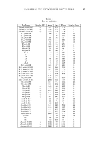
![30 PIERRE BONAMI, MUSTAFA KILINÇ, AND JEFF LINDEROTH
satisfied by open facilities. The objective is to minimize the sum of the fixed
cost for operating facilities and the shipping cost which is proportional to
the square of the quantity delivered to each customer.
All test problems are available in AMPL and GAMS formats and are
available from the authors upon request. In our experiments, α−ECP,
DICOPT, and SBB are tested through the GAMS interface, while Bonmin,
FilMINT and MINLP BB are tested through AMPL.
6.2. Computational results. The computational experiments have
been run on a cluster of identical 64-bit Intel Xeon microprocessors clocked
at 2.67 GHz, each with 3 GB RAM. All machines run the Red Hat En-
terprise Linux Server 5.3 operating system. A three hour time limit is
enforced. The computing times used in our comparisons are the wall-clock
times (including system time). All runs were made on processors dedicated
to the computation. Wall-clock times were used to accurately account for
system overhead incurred by file I/O operations required by the SBB solver.
For example, on the problem FLay05M, SBB reports a solution time of 0.0
seconds for 92241 nodes, but the wall-clock time spent is more than 17
minutes.
Table 3 summarizes the performance of the solvers on the 48 problems
of the test set. The table lists for each solver the number of times the opti-
mal solution was found, the number of times the time limit was exceeded,
the number of times the node limit exceeded, the number of times an error
occurred (other than time limit or memory limit), the number of times
the solver is fastest, and the arithmetic and geometric means of solution
times in seconds. When reporting aggregated solution times, unsolved or
failed instances are accounted for with the time limit of three hours. A
performance profile [40] of solution time is given in Figure 1. The detailed
performance of each solver on each test instance is listed in Table 4.
There are a number of interesting observations that can be made from
this experiment. First, for the instances that they can solve, the solvers
DICOPT and α-ECP tend to be very fast. Also, loosely speaking, for each
class of instances, there seems to be one or two solvers whose performance
dominates the others, and we have listed these in Table 2.
Table 2
Subjective Rating of Best Solver on Specific Instance Families.
Instance Family Best Solvers
Batch DICOPT
CLay, FLay, sssd FilMINT, MINLP BB
Fo, RSyn, Syn DICOPT, α-ECP
SLay MINLP BB
uflquad Bonmin (B-BB)](https://image.slidesharecdn.com/11816511-250518184510-47b062f0/85/Mixed-Integer-Nonlinear-Programming-The-Ima-Volumes-In-Mathematics-And-Its-Applications-2012th-Edition-Leyffer-54-320.jpg)