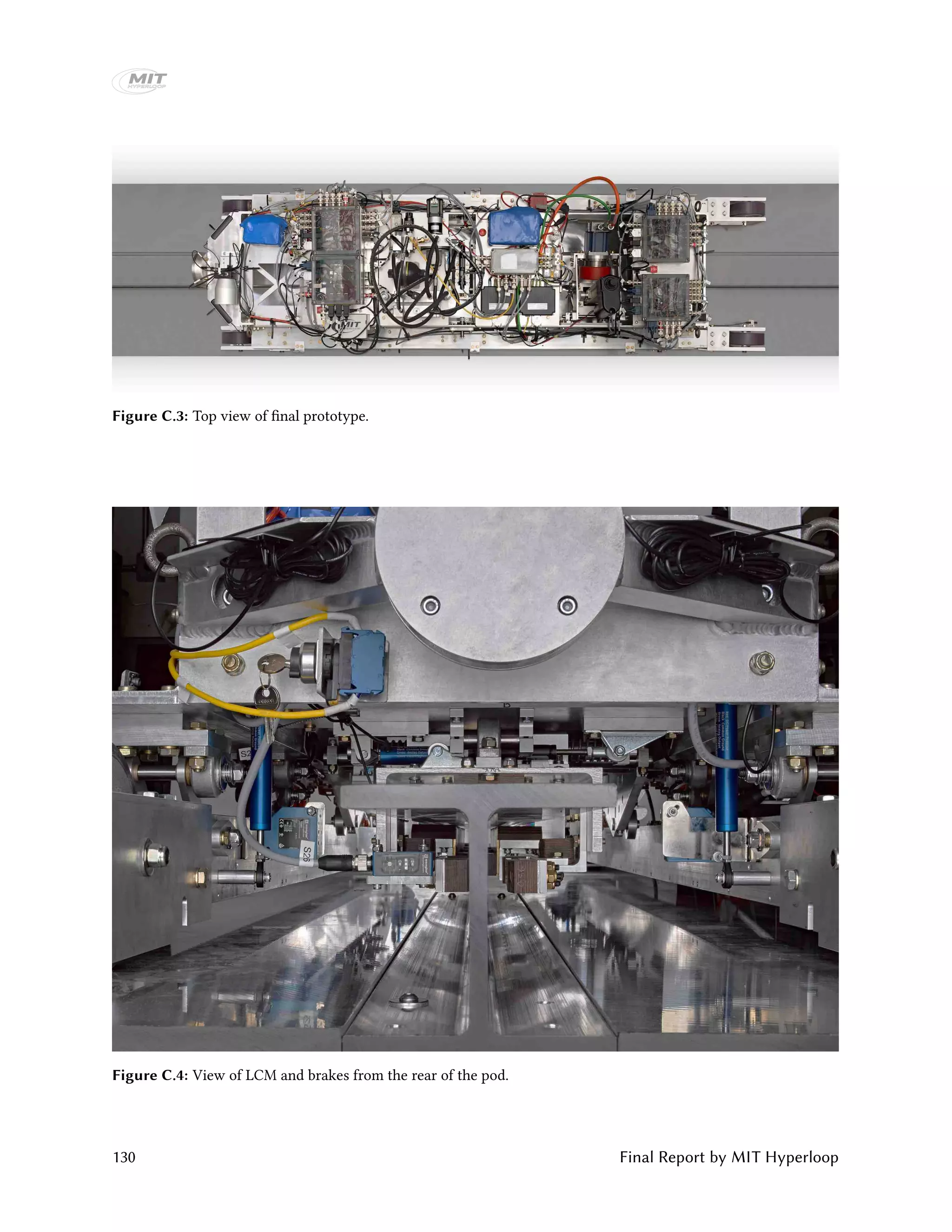
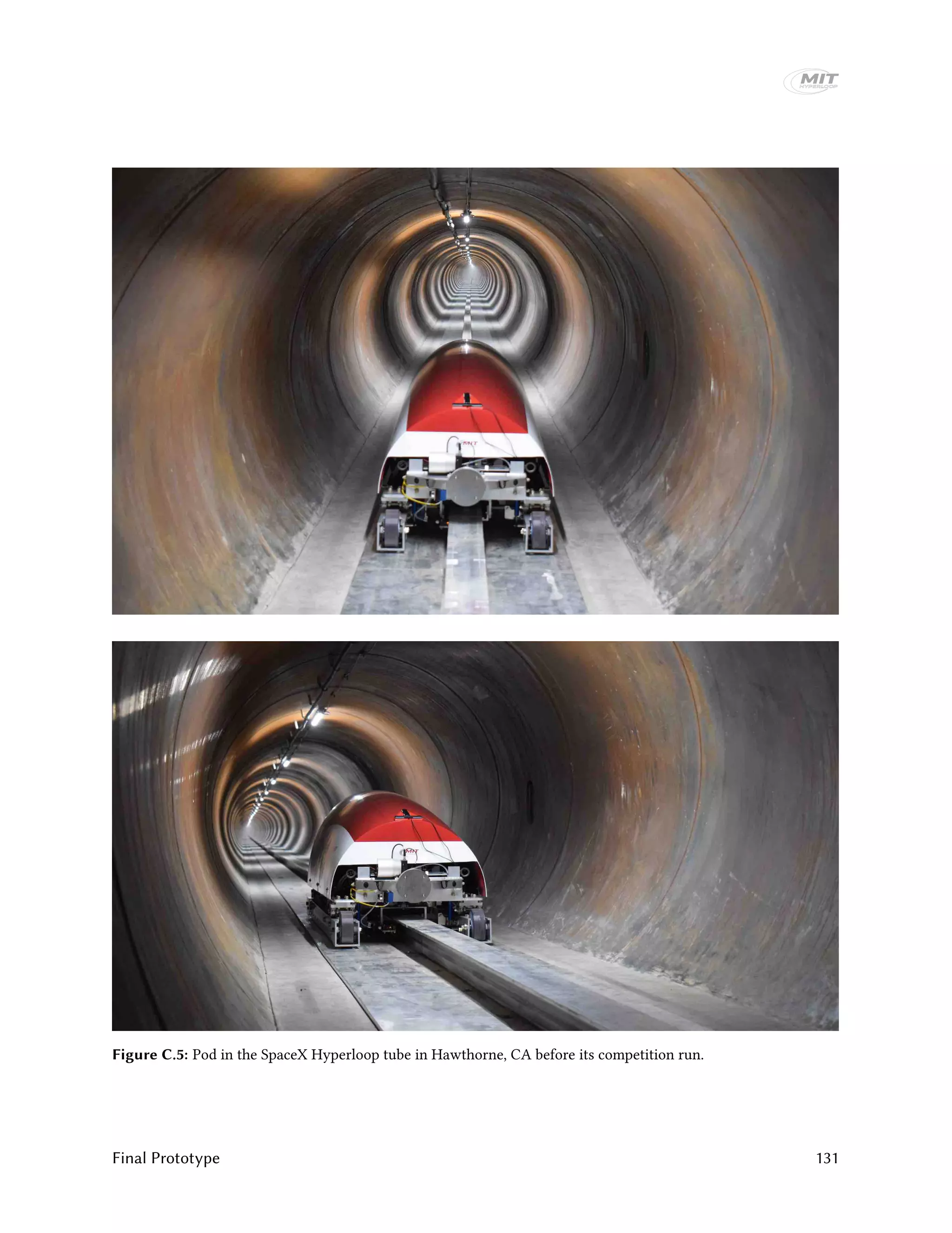
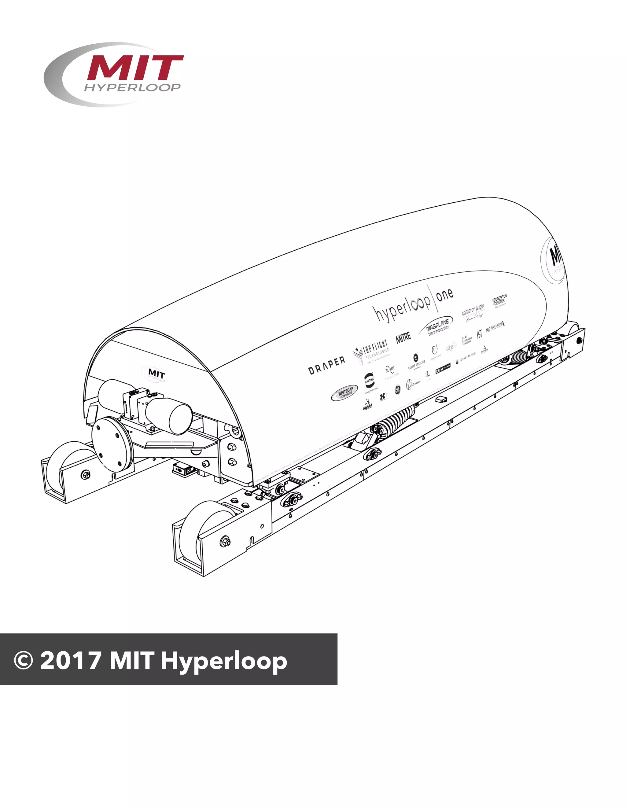
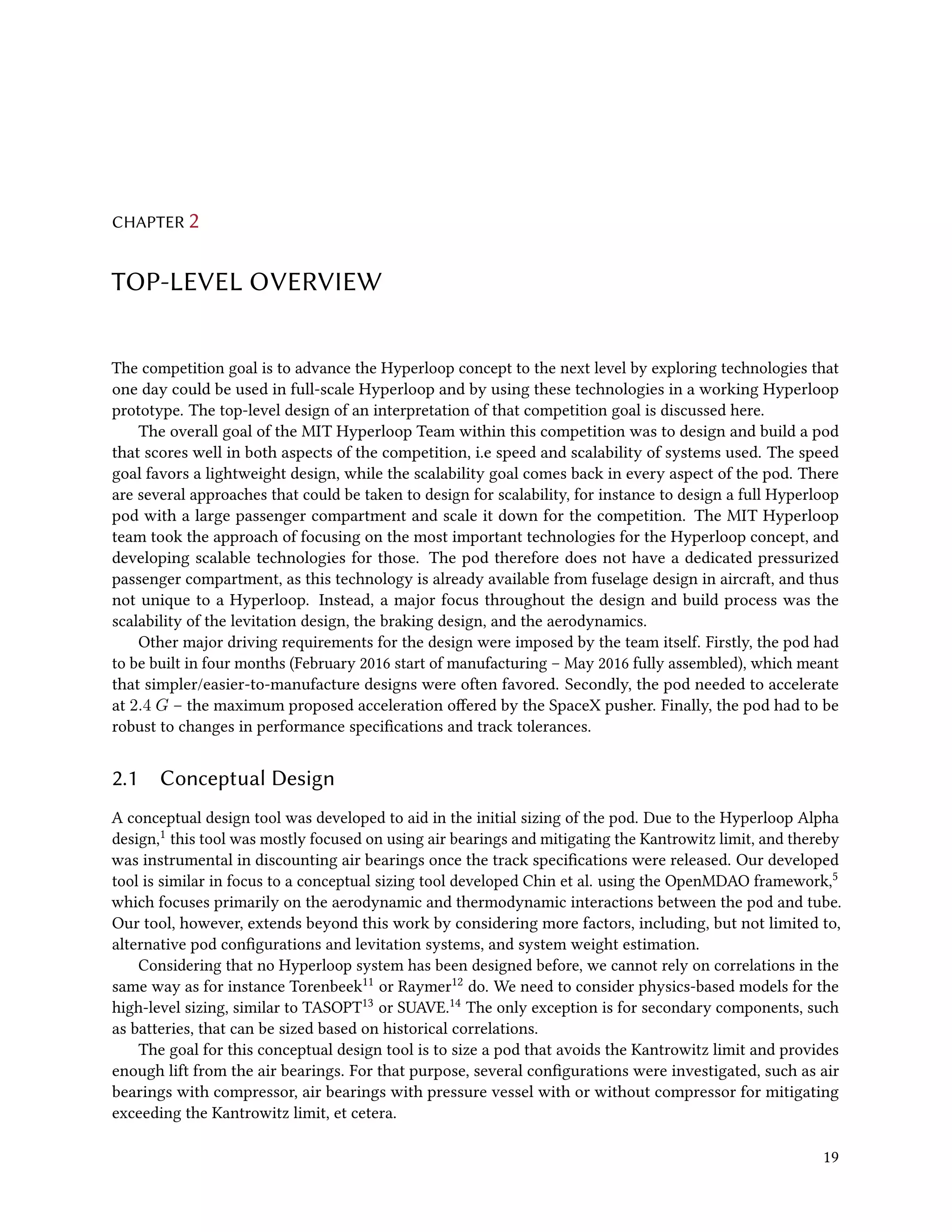
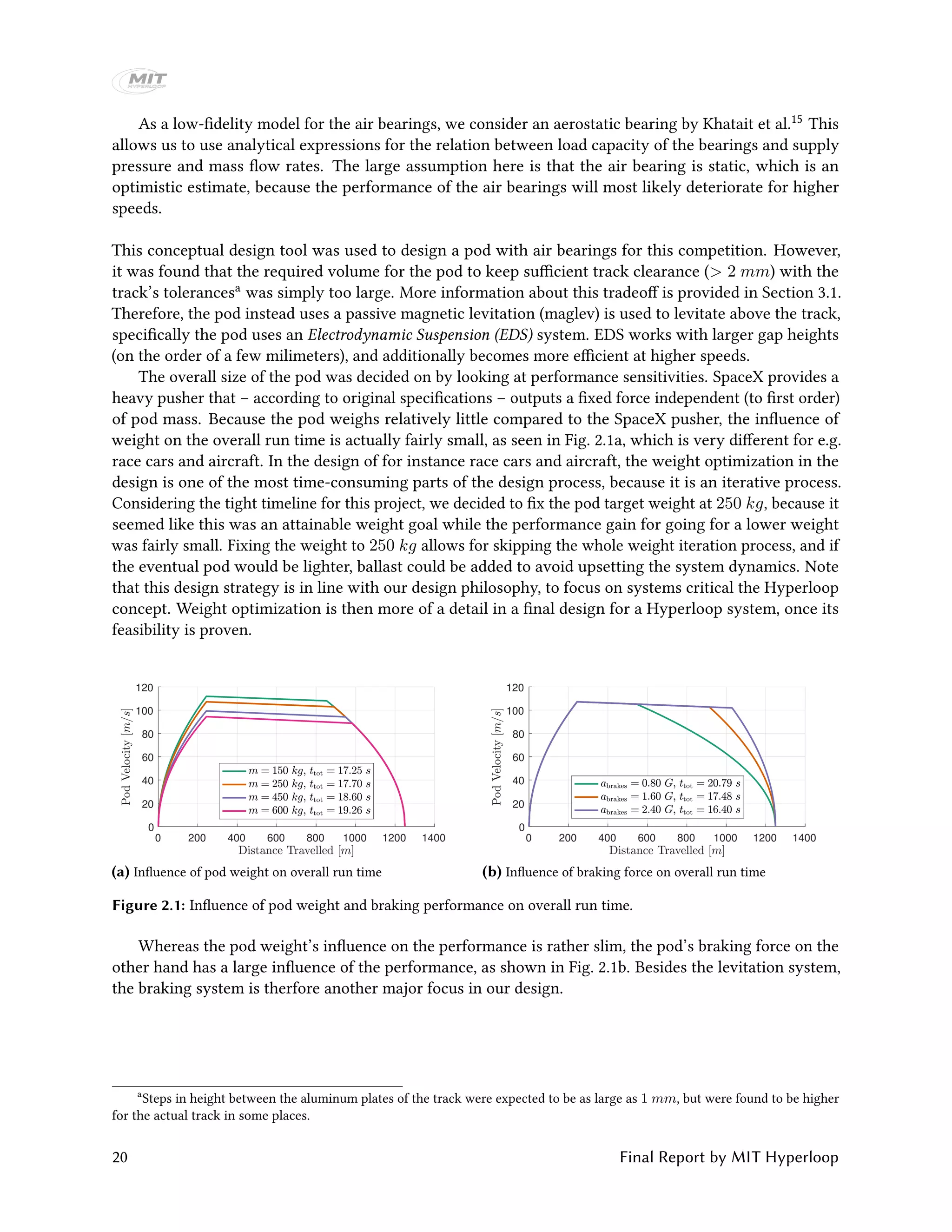
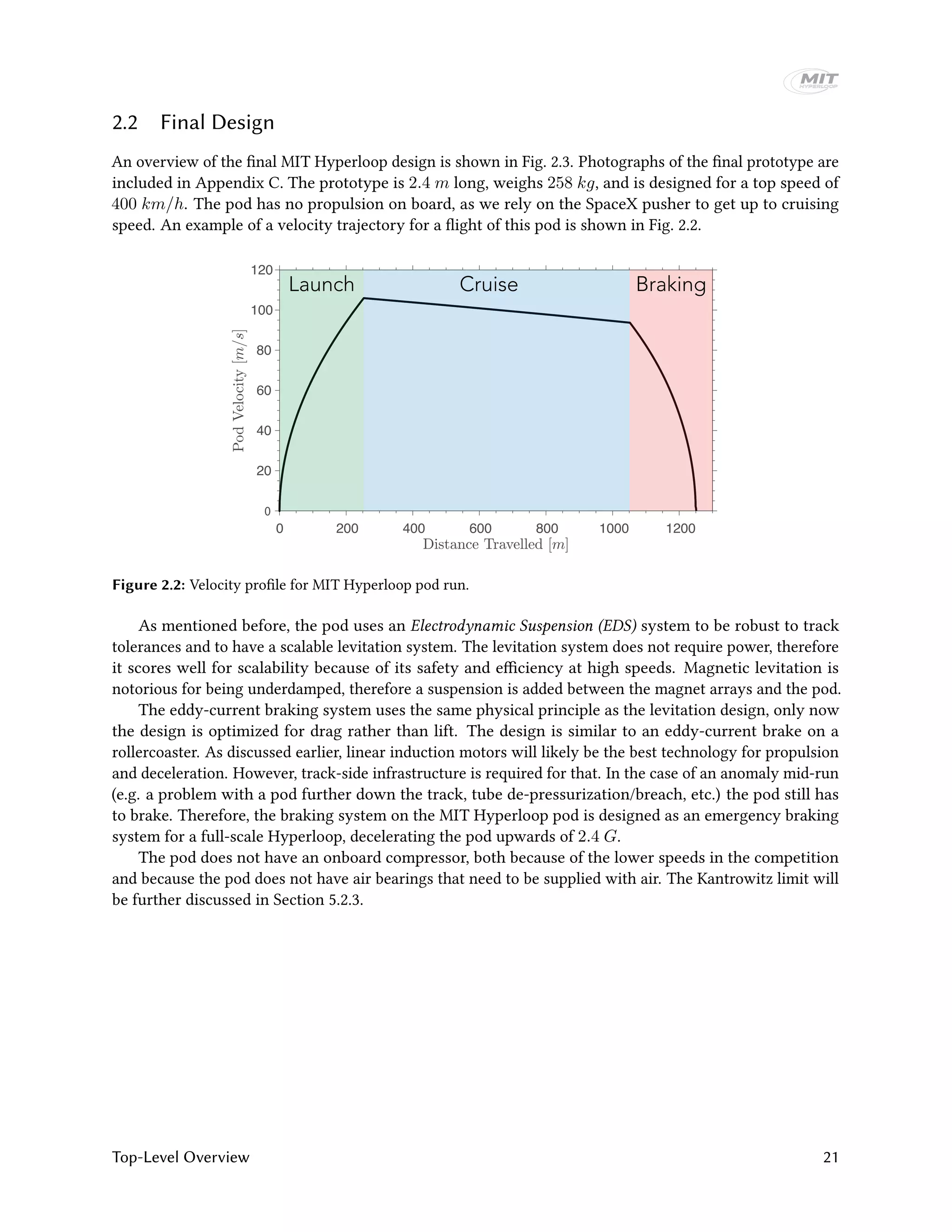
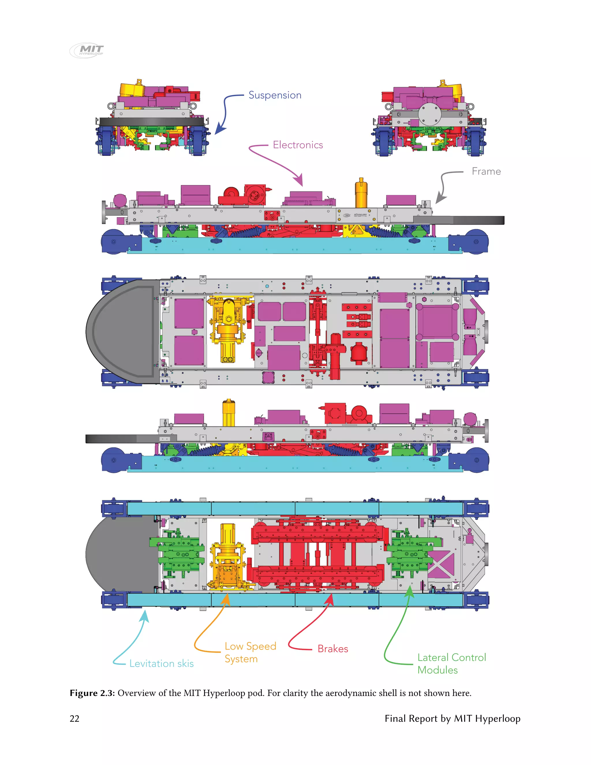
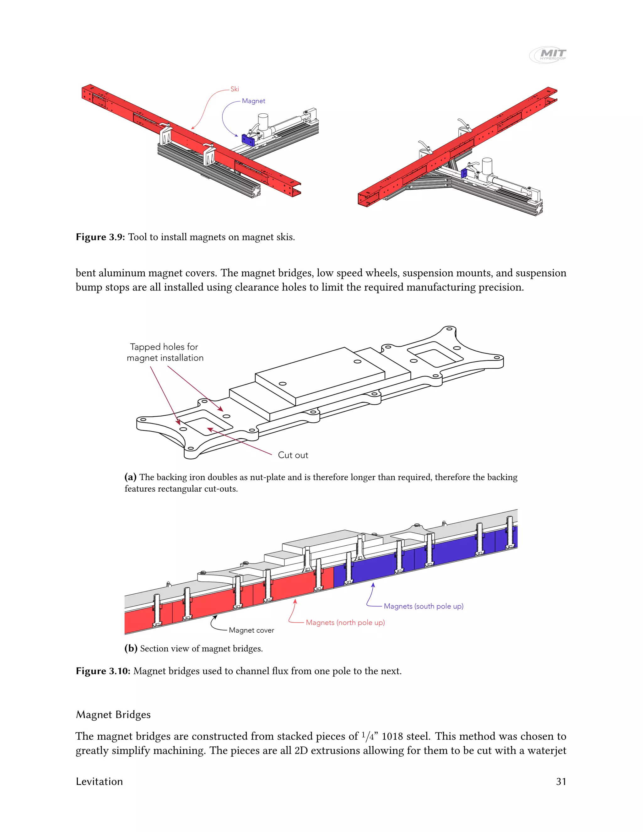
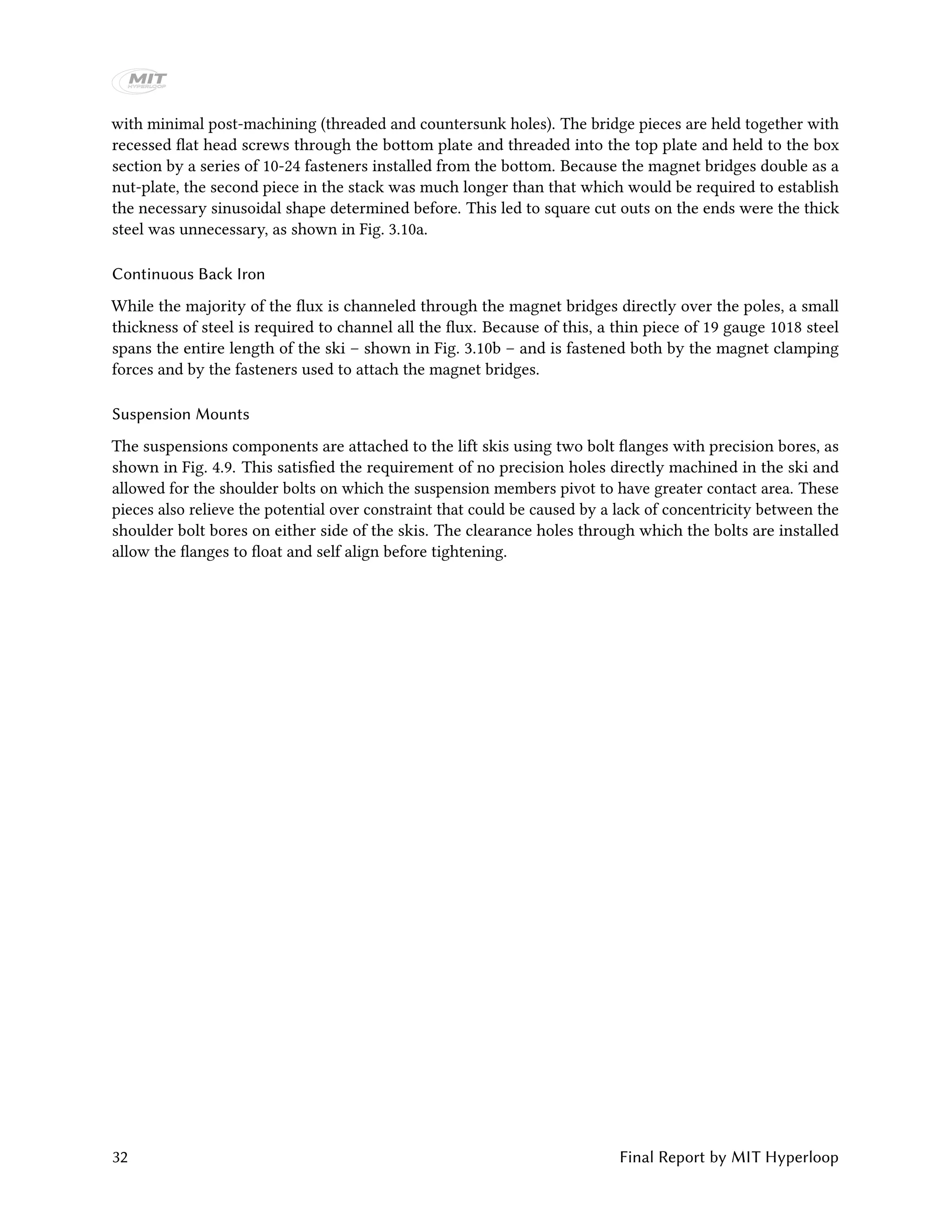
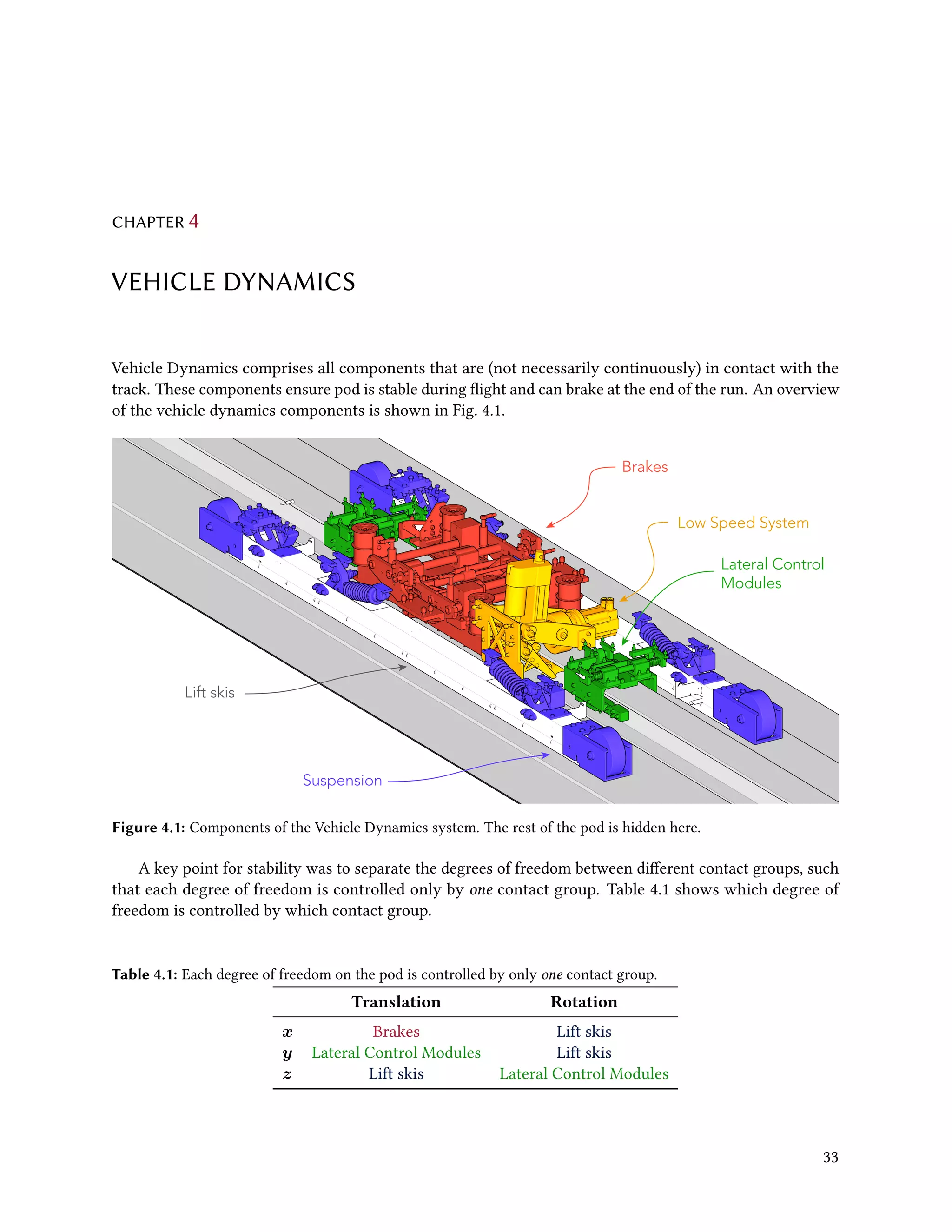
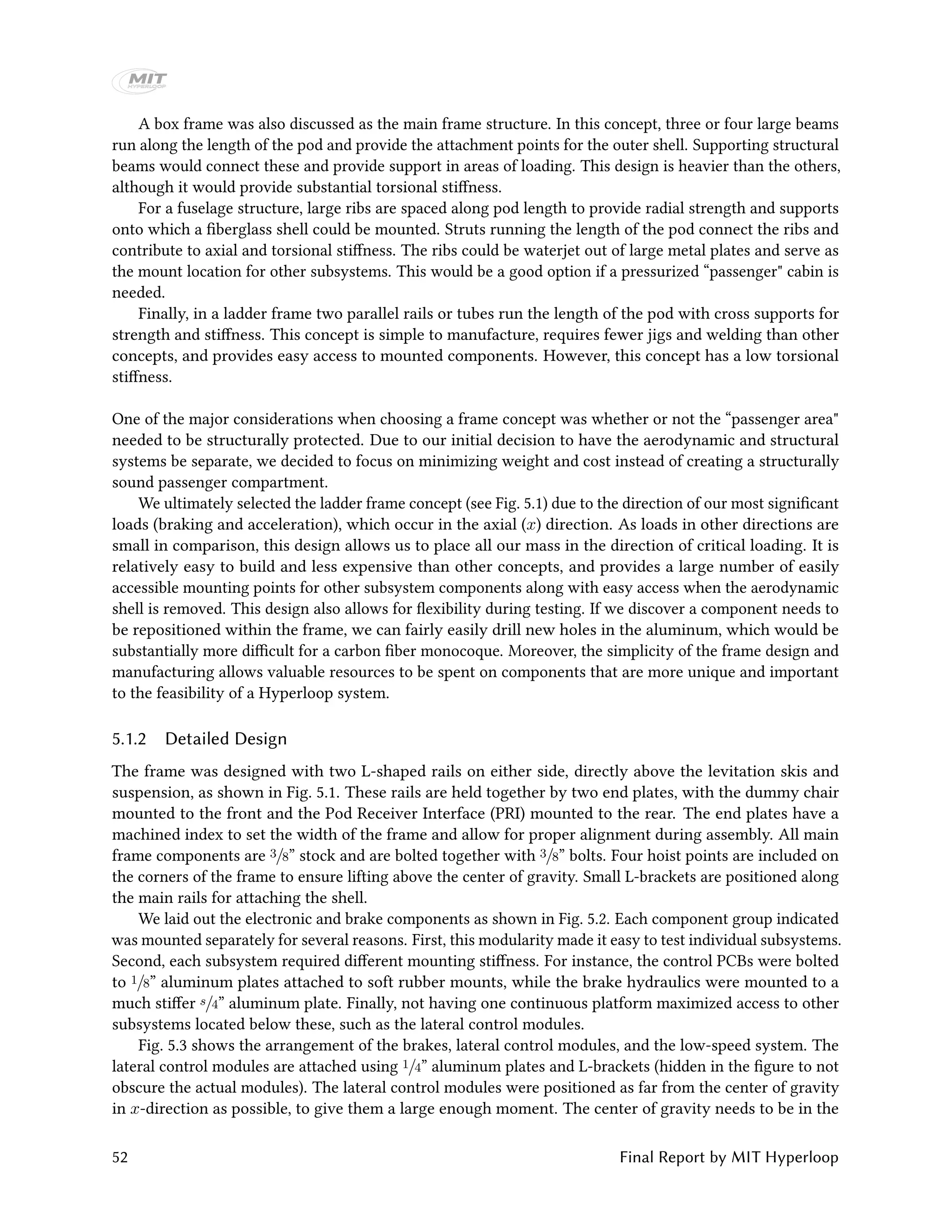
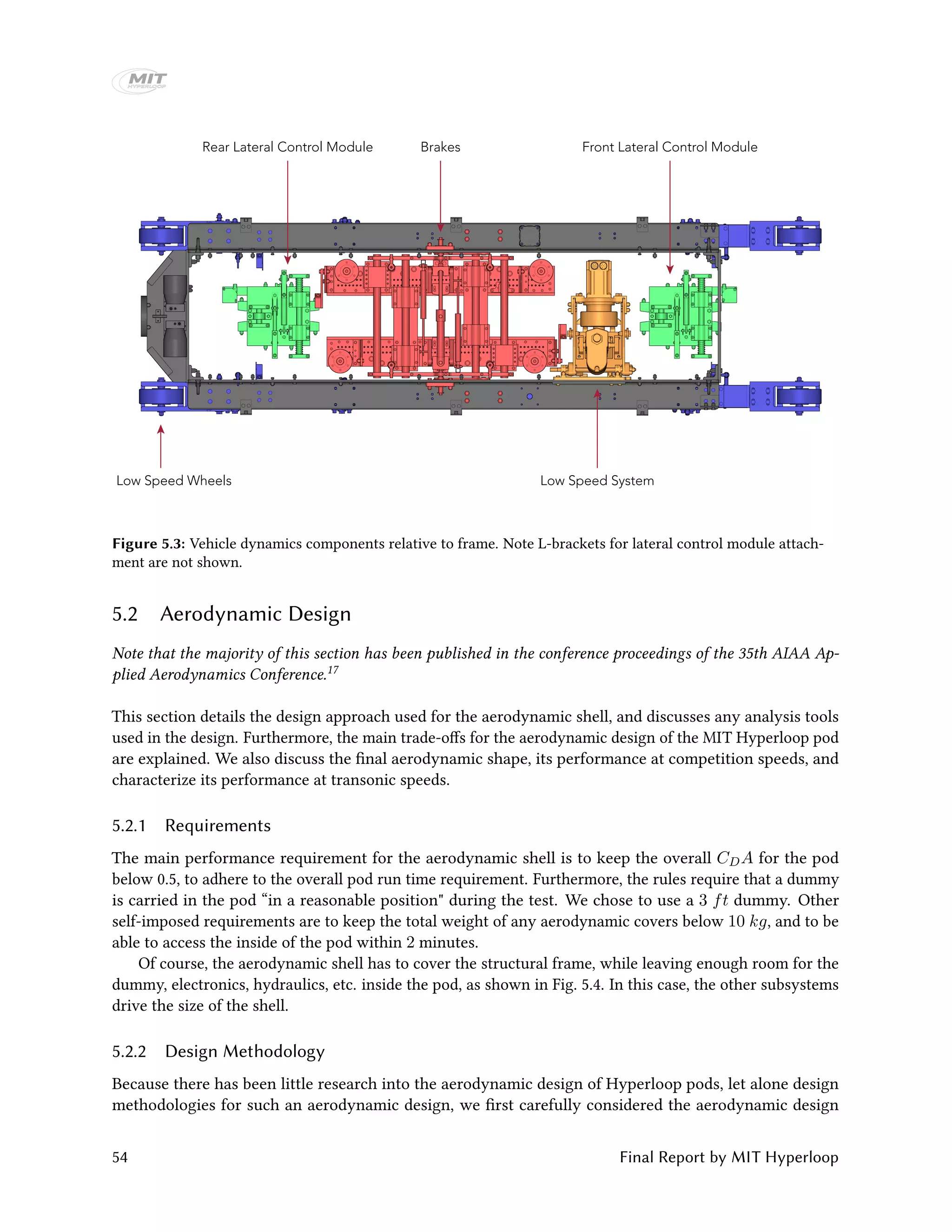
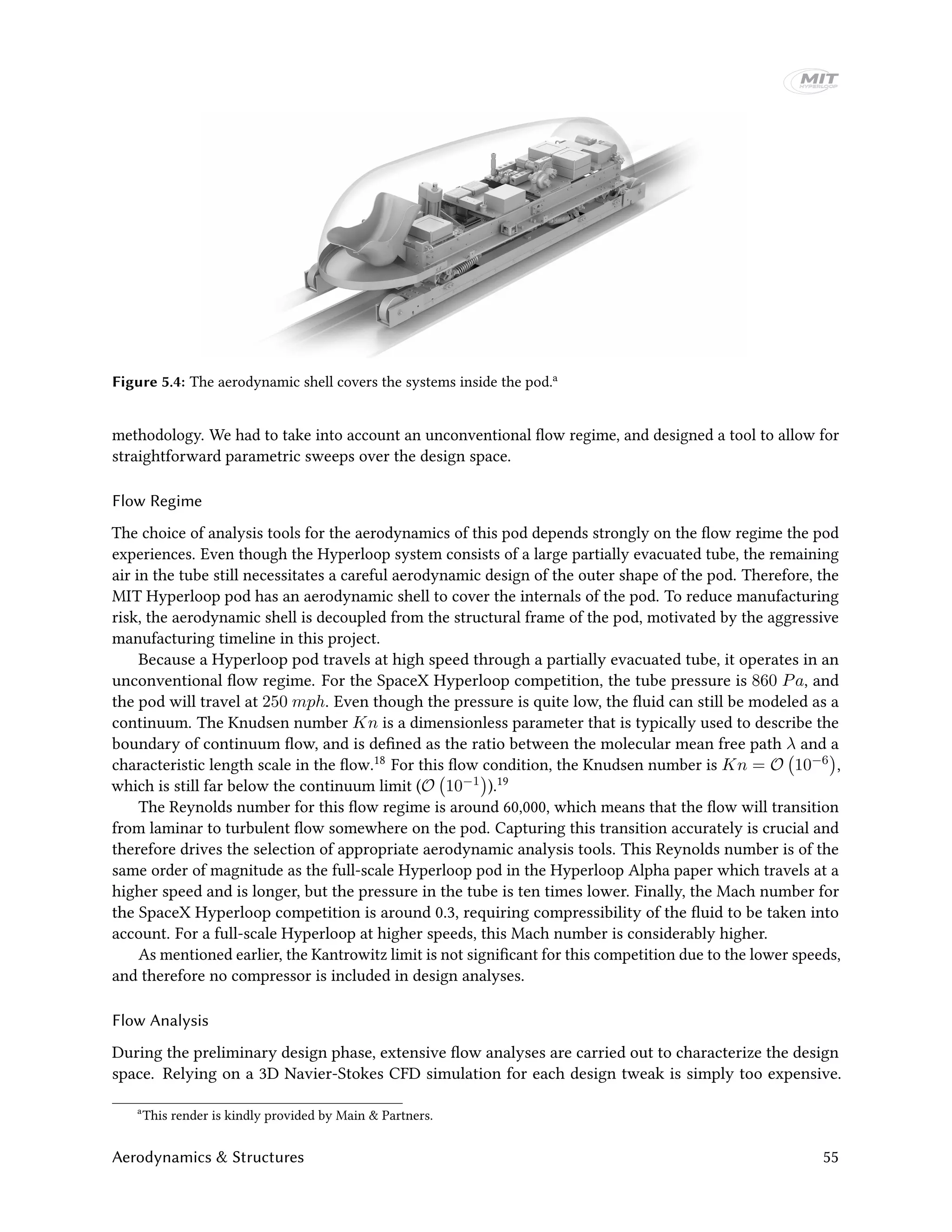
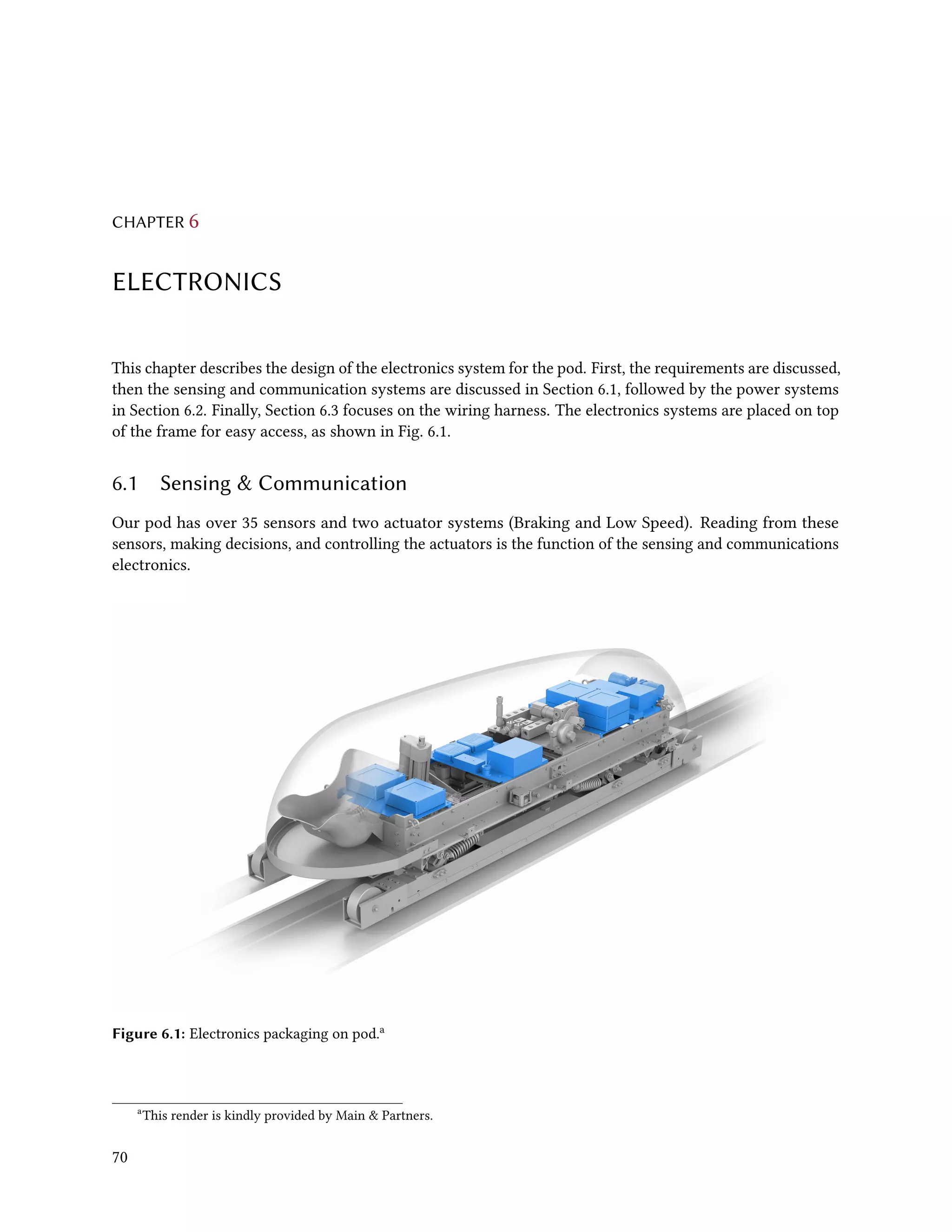
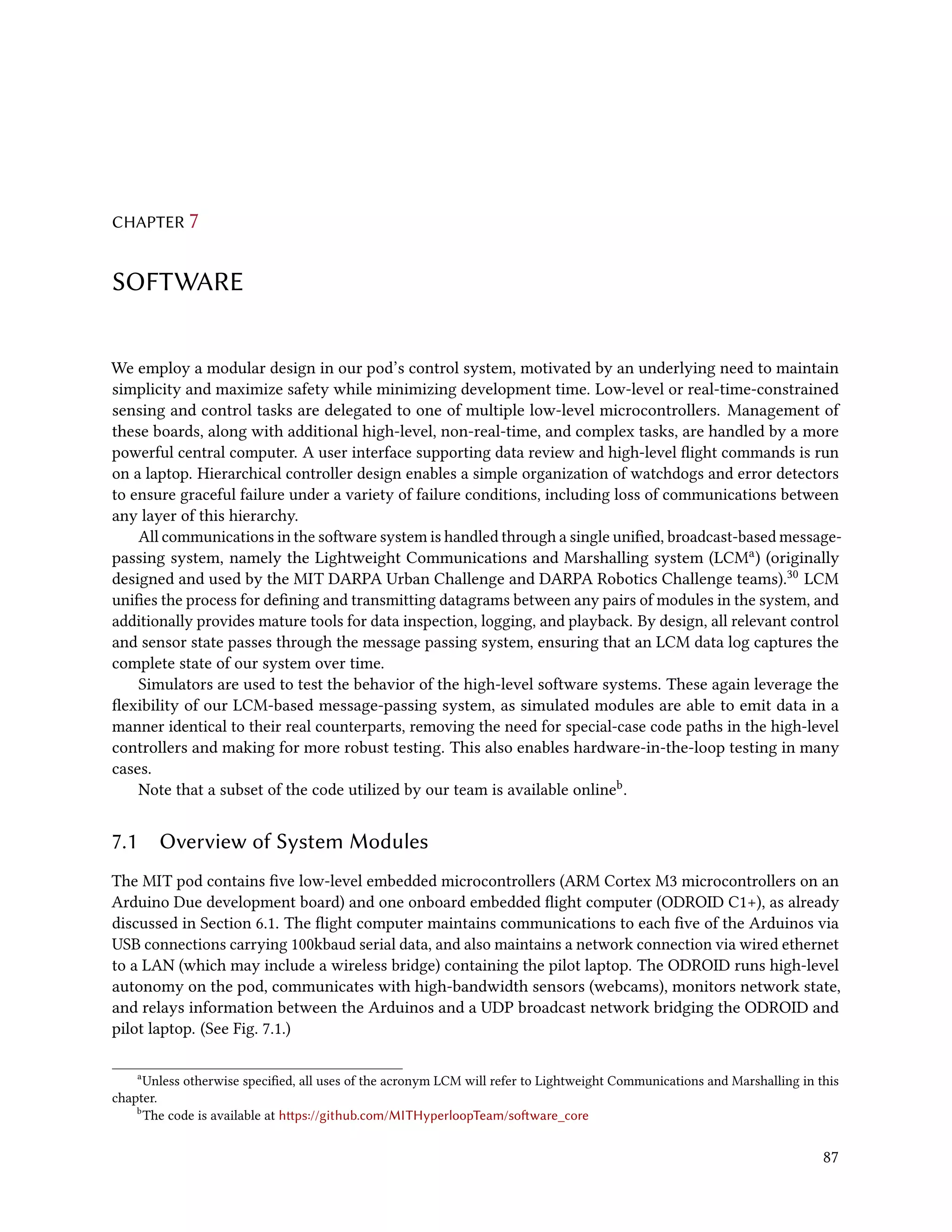
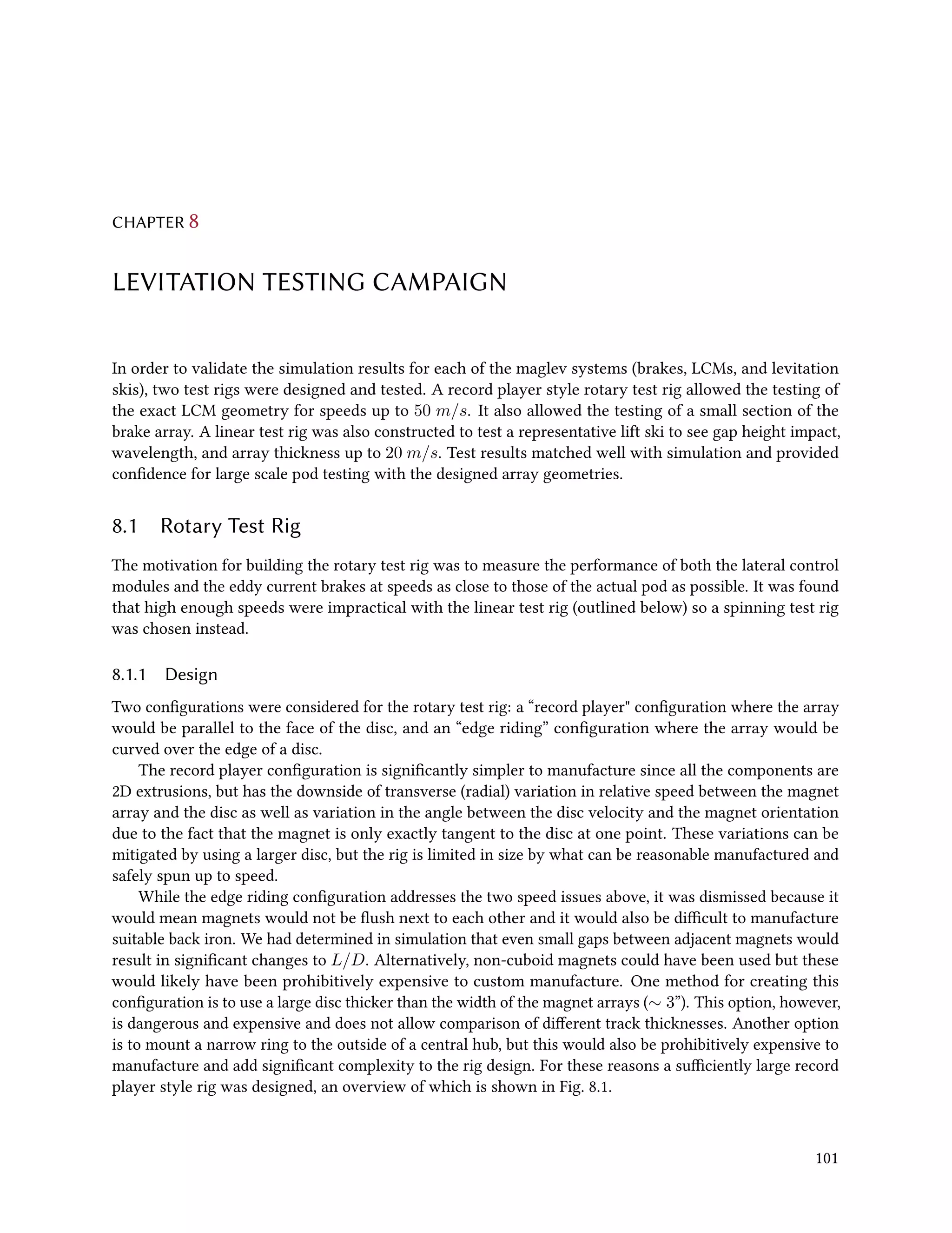
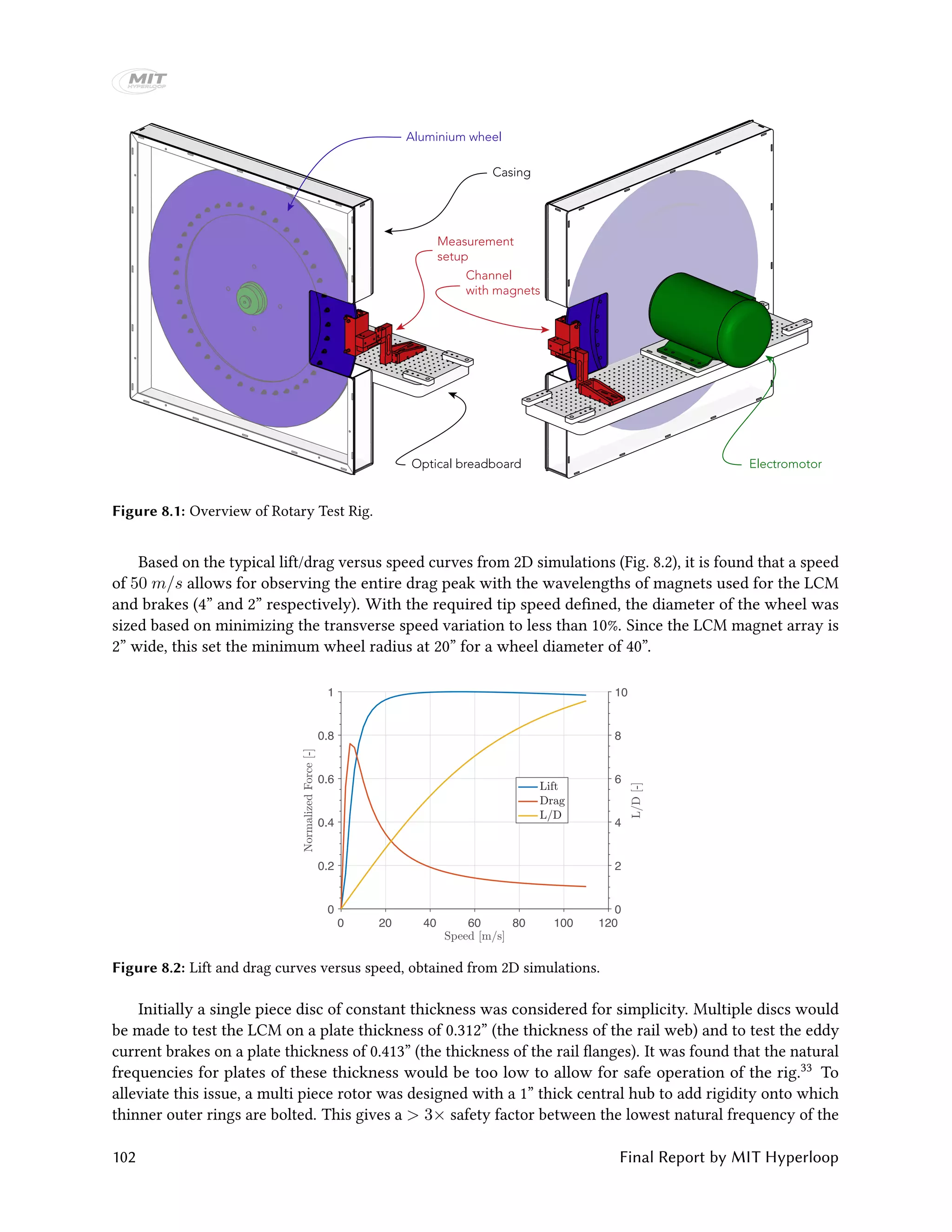
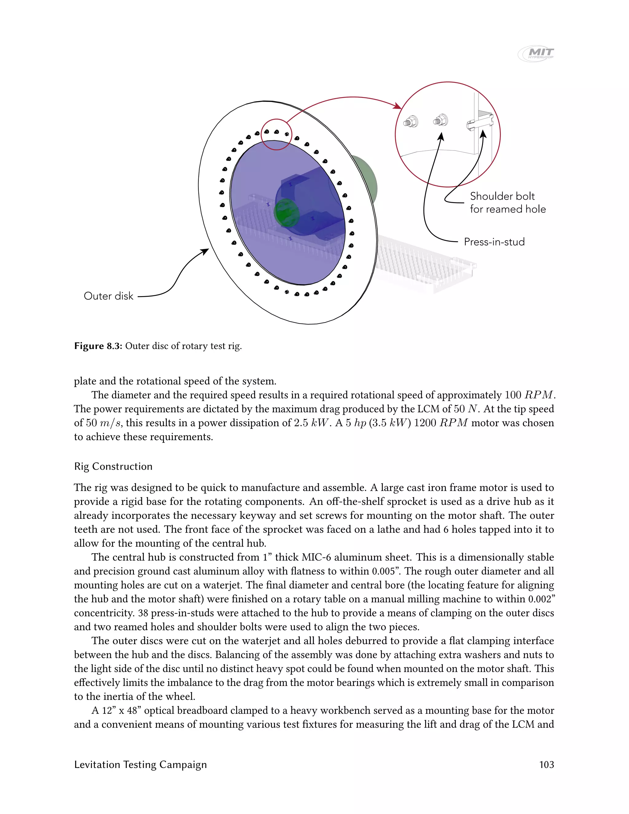
The MIT Hyperloop team designed and built a scaled Hyperloop pod prototype to compete in the SpaceX Hyperloop competition from 2015-2017. Their pod used an electrodynamic suspension maglev system for levitation and braking. It had lateral control modules to provide stability and brakes that could slow the pod down at over 2 Gs. Extensive testing was conducted on the levitation and vibration systems. At the competition, the pod demonstrated stable levitation in a vacuum environment, won the Safety & Reliability award, and placed third in Design & Construction. The report provides details on the pod design, manufacturing, and competition performance.


![THE MIT HYPERLOOP TEAM IS GRATEFUL FOR THE GENEROUS SUPPORT FROM ITS SPONSORS
[ H I G H P E R F O R M A N C E C O M P U T I N G I N T H E C L O U D ]
[ H I G H P E R F O R M A N C E C O M P U T I N G I N T H E C L O U D ]](https://image.slidesharecdn.com/mithyperloopfinalreport2017public-191204174448/75/Mit-hyperloop-final_report_2017_public-8-2048.jpg)


![MIT HL
M∞ [−]
0.1 0.2 0.3 0.4 0.5 0.6 0.7 0.8 0.9
Apod/Atube[−]
0.1
0.2
0.3
0.4
0.5
0.6
0.7
0.8
0.9
Kantrowitz limit
Mext[−]
0.2
0.3
0.4
0.5
0.6
0.7
0.8
0.9
Figure 5.7: Area ratio (pod-to-tube) versus Mach number. Mext is the maximum Mach number of the flow around
the pod – if M = 1 the flow is exactly choked. The red line indicates the Kantrowitz limit.
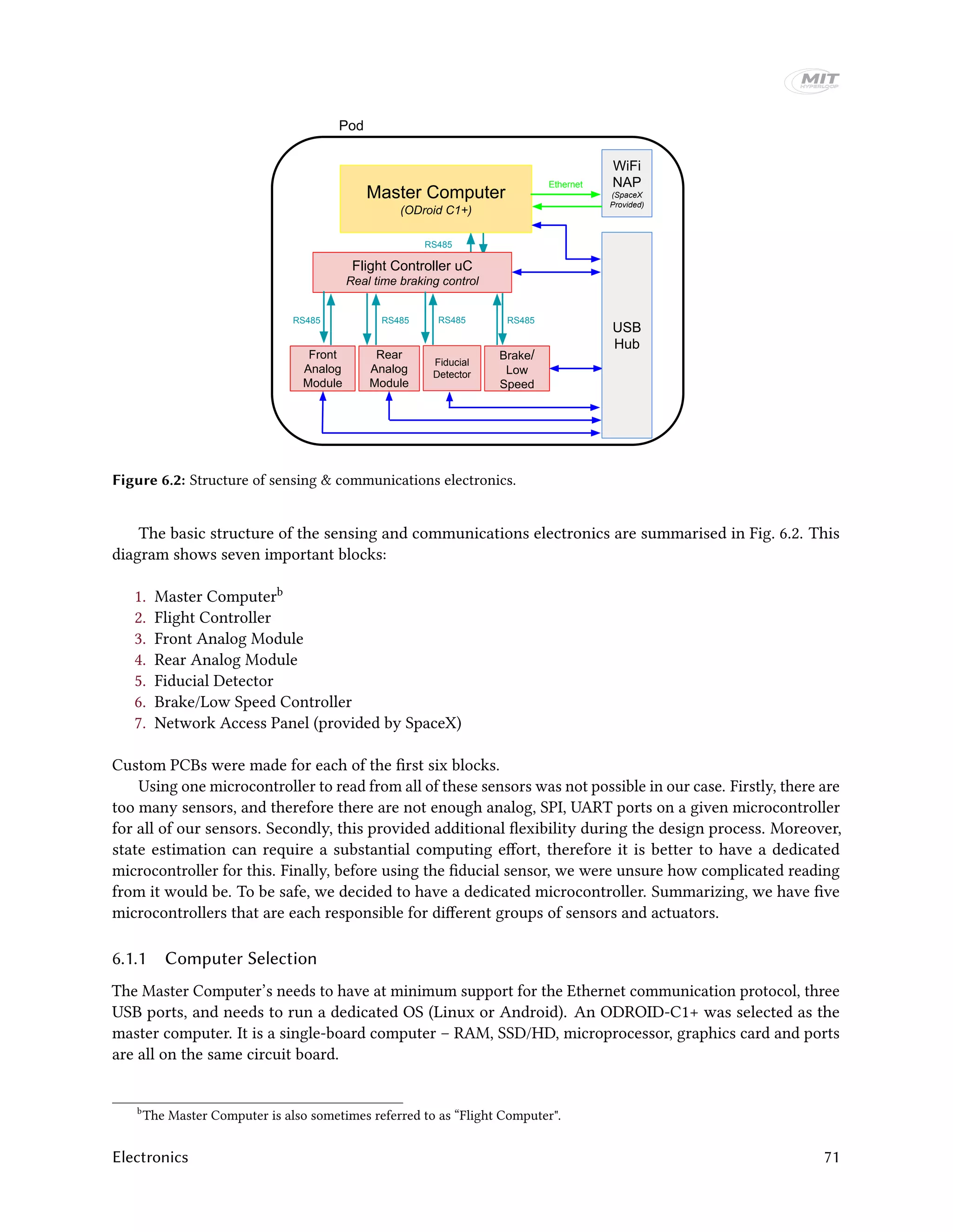
for the SpaceX Hyperloop competition. Fig. 5.7 shows the variation of the external Mach number to the
pod-to-tube ratio and the freestream Mach number. The external Mach number is the maximum Mach
number of the flow around the pod, the flow is choked when that external Mach number equals 1.0. Fig. 5.7
clearly shows that for a reasonably sized pod without a compressor, the Kantrowitz limits the speed of
the pod without an additional drag increase. At an area ratio of 0.3 and a Mach number of 0.3, the flow
around the pod is not even close to choking, as seen in Fig. 5.7. Because compressors also have a large risk
associated with them in terms of design, manufacturing, and cost, the MIT Hyperloop team decided not to
use a compressor.
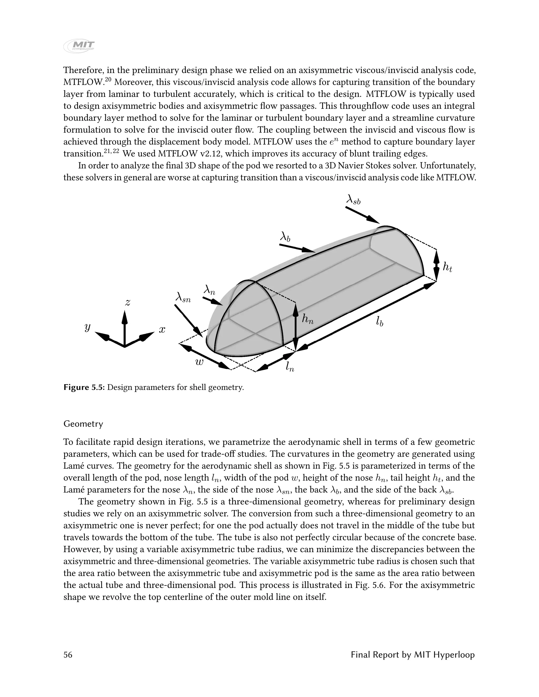
Axisymmetric design
First, an axisymmetric aerodynamic shell was designed using MTFLOW.20 All of the results in this section
are generated using MTFLOW. In the aerodynamic design we relied on sweeps over the design parameters
in Fig. 5.5, rather than going for a purely numerical optimization method. The main reason for this was
to gain more physical insight in this design problem with a large unexplored design space, and to use
constraints that would be harder to capture in mathematical statements. Additionally, this allowed for a
more aggressive design schedule.
Cp
1
0.75
0.5
0.25
0
-0.25
-0.5
-0.75
-1
-1.25
-1.5
-1.75
-2
Figure 5.8: Laminar flow separation on a Hyperloop pod at a Reynolds number Re = 60, 000 and Mach number
M∞ = 0.3. The boundary layer and wake are indicated in gray.
58 Final Report by MIT Hyperloop](https://image.slidesharecdn.com/mithyperloopfinalreport2017public-191204174448/75/Mit-hyperloop-final_report_2017_public-58-2048.jpg)
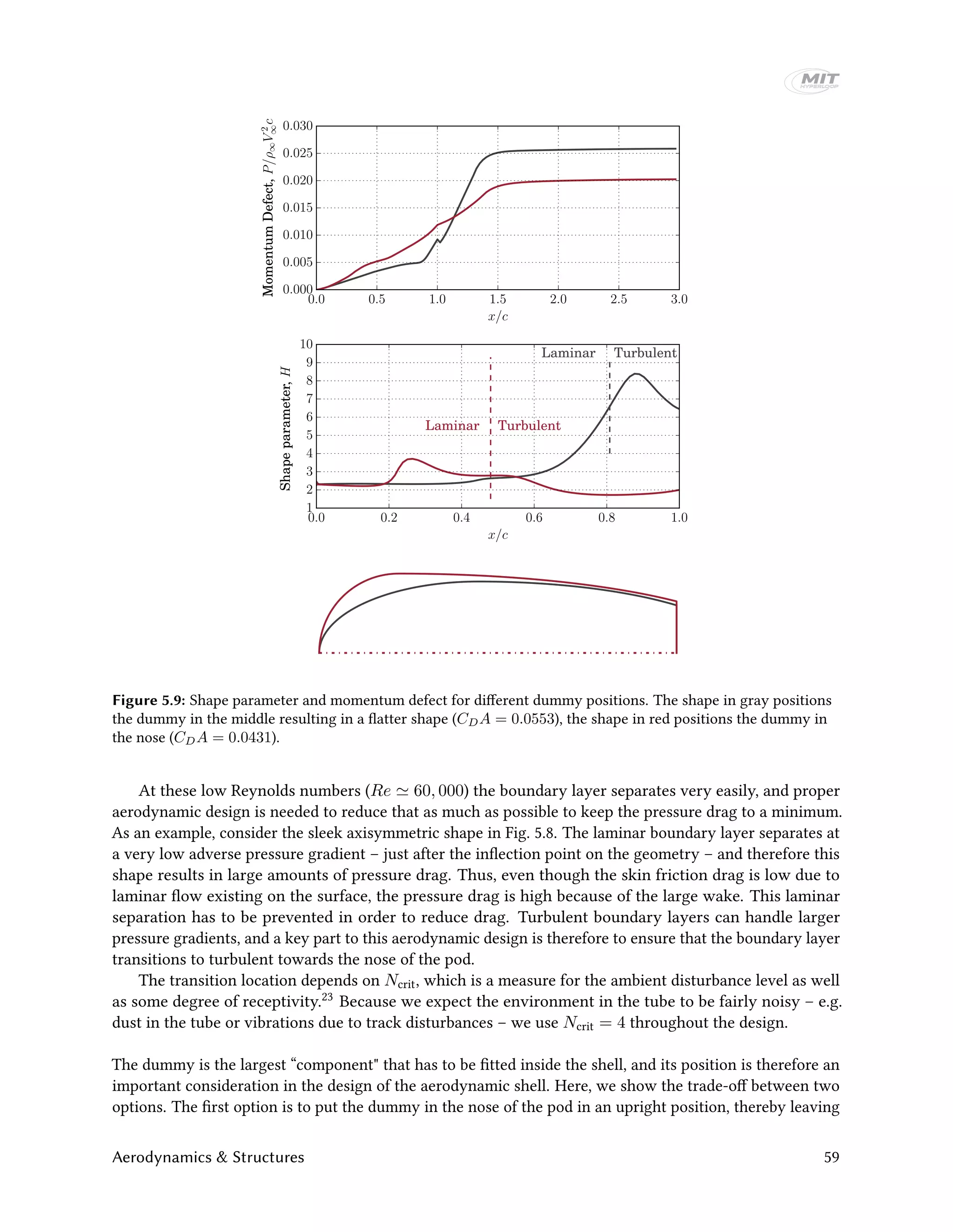
![more room for components towards the rear of the pod but resulting in a higher nose. The second option is
to lay the dummy more flat over the components inside the pod, thereby reducing the height of the pod
and allowing for a more gradual ramp-up to the highest point of the pod.
Fig. 5.9 shows the results for both of these shapes. For the shape with the dummy in the nose, the
boundary layer transitions much closer to the nose, therefore delaying separation and reducing pressure
drag. For the shape with the dummy laying flat, the laminar boundary layer separates close to the highest
point on the pod, resulting in large pressure drag. Therefore, even though the shape with the dummy in
the nose has a larger cross-sectional area, the drag is lower. The reason for this is the blunt nose which is
known to promote early transition.24
Several different sweeps over design parameters have been performed during the design stage, although
only a few of them are discussed here. Fig. 5.10 shows the influence of the nose Lamé parameter and the
tail height on the drag coefficient. When the nose is too shallow (e.g. λn = 1.5) transition will occur later
on the pod and more pressure drag results. However, too blunt of a nose increases the curvature on the
highest point of the nose, which also induces separation. For the tail height, the higher the tail the higher
the pressure drag. However, too low of tail does not add any benefit because the flow separates anyway.
1.0 1.5 2.0 2.5 3.0 3.5
Nose Lam´e parameter, λN
0.000
0.010
0.020
0.030
0.040
0.050
0.060
0.070
0.080
CDA
Total
Pressure
Friction
(a) Nose bluntness influence on CDA for tail height of 12 in.
11 12 13 14 15 16 17 18 19 20
Tail height, [in]
0.000
0.050
0.100
0.150
0.200
0.250
CDA
Total
Pressure
Friction
(b) Tail height influence on CDA for nose Lamé parameter λN = 2.0.
Figure 5.10: Nose bluntness and tail height influence on drag for axisymmetric pod.
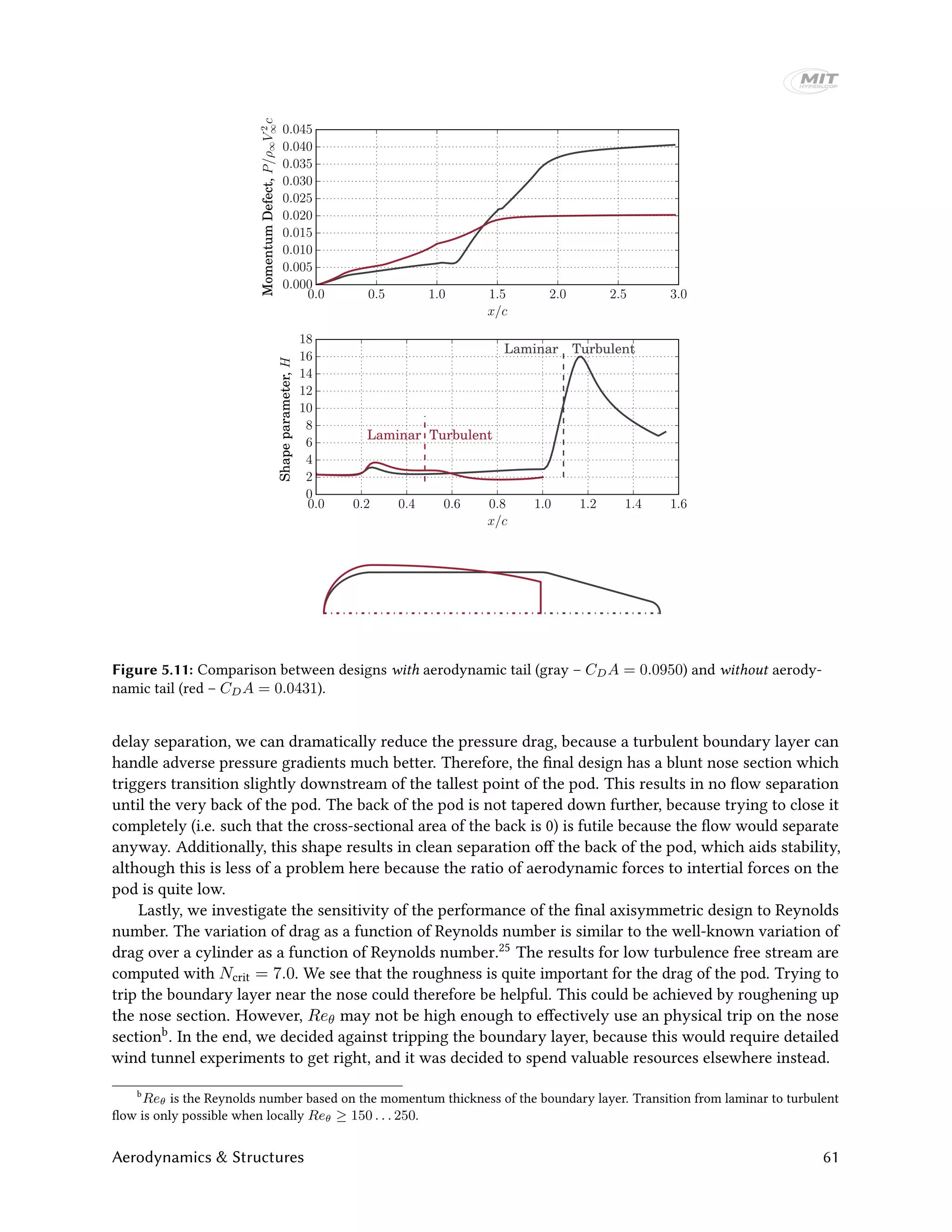
We also investigate the use of an aerodynamic tail section to reduce drag. The idea is to keep a straight
section of most of the components on the pod to provide maximum payload capacity, and then add a
lightweight aerodynamic tail section to keep drag to a minimum. We compare such a design to our final
design in Fig. 5.11. The concept with an aerodynamic tail has a smaller cross-sectional diameter to keep the
internal volume (excluding tail) similar. The momentum defect on the pod surface is much better for the
pod with an aerodynamic tail because there is no adverse pressure gradient on the pod. However, the flow
separates as soon as the aerodynamic tail is reached, dramatically increasing the momentum defect. The
large increase in pressure drag therefore renders the aerodynamic tail useless.
The flow field around the final geometry is shown in Fig. 5.12. As mentioned several times, if we can
60 Final Report by MIT Hyperloop](https://image.slidesharecdn.com/mithyperloopfinalreport2017public-191204174448/75/Mit-hyperloop-final_report_2017_public-60-2048.jpg)
![Cp
1
0.5
0
-0.5
-1
-1.5
-2
-2.5
-3
Figure 5.12: Flow field around the final axisymmetric design at Reynolds number Re = 60, 000 and Mach num-
ber M∞ = 0.3. The boundary layer and wake are indicated in gray.
50000 100000 150000 200000 250000
Reynolds number, Re
0.010
0.020
0.030
0.040
0.050
CDA
(a) Drag coefficient versus Reynolds number
500 1000 1500 2000 2500 3000 3500 4000
Tube pressure, p [Pa]
0
2
4
6
8
10
Drag,D[N]
Total (Ncrit = 4.0)
Pressure (Ncrit = 4.0)
Friction (Ncrit = 4.0)
Total (Ncrit = 7.0)
(b) Drag versus tube pressure. Note that the tube pressure is pro-
portional to Reynolds number, because the pod velocity and tube
temperature are kept constant here.
0.0 0.5 1.0 1.5 2.0 2.5 3.0
x/c
0.000
0.005
0.010
0.015
0.020
0.025
MomentumDefect,P/ρ∞V2
∞c
(c) Momentum defect
0.0 0.2 0.4 0.6 0.8 1.0
x/c
0
1
2
3
4
5
Shapeparameter,H
50k
80k
110k
140k
170k
200k
230k
250k
(d) Shape parameter over body
Figure 5.13: Sensitivity of final axisymmetric shape to Reynolds number.
Final Three-Dimensional Shape
To generate the three-dimensional shape from the final axisymmetric shape, the axisymmetric shape
is used as the centerline for the pod. The other design parameters from Fig. 5.5 are determined from
packaging constraints with the other subsystems (e.g. structural frame, electronics, hydraulics, etc.). We
study the performance of this design using STAR-CCM+. For these simulations we solve the laminar Navier-
Stokes equations on a very fine grid (2.58 million cells). Adding a turbulence model would overestimate
the transition location to be too far upstream and therefore underestimate separation to occur too far
downstream. These simulations have to be unsteady because flow separation off the back is an inherently
unsteady phenomenon. Total flow conditions (total temperature, total pressure) are set at the inlet to the
domain and a pressure outlet is used at the outflow.
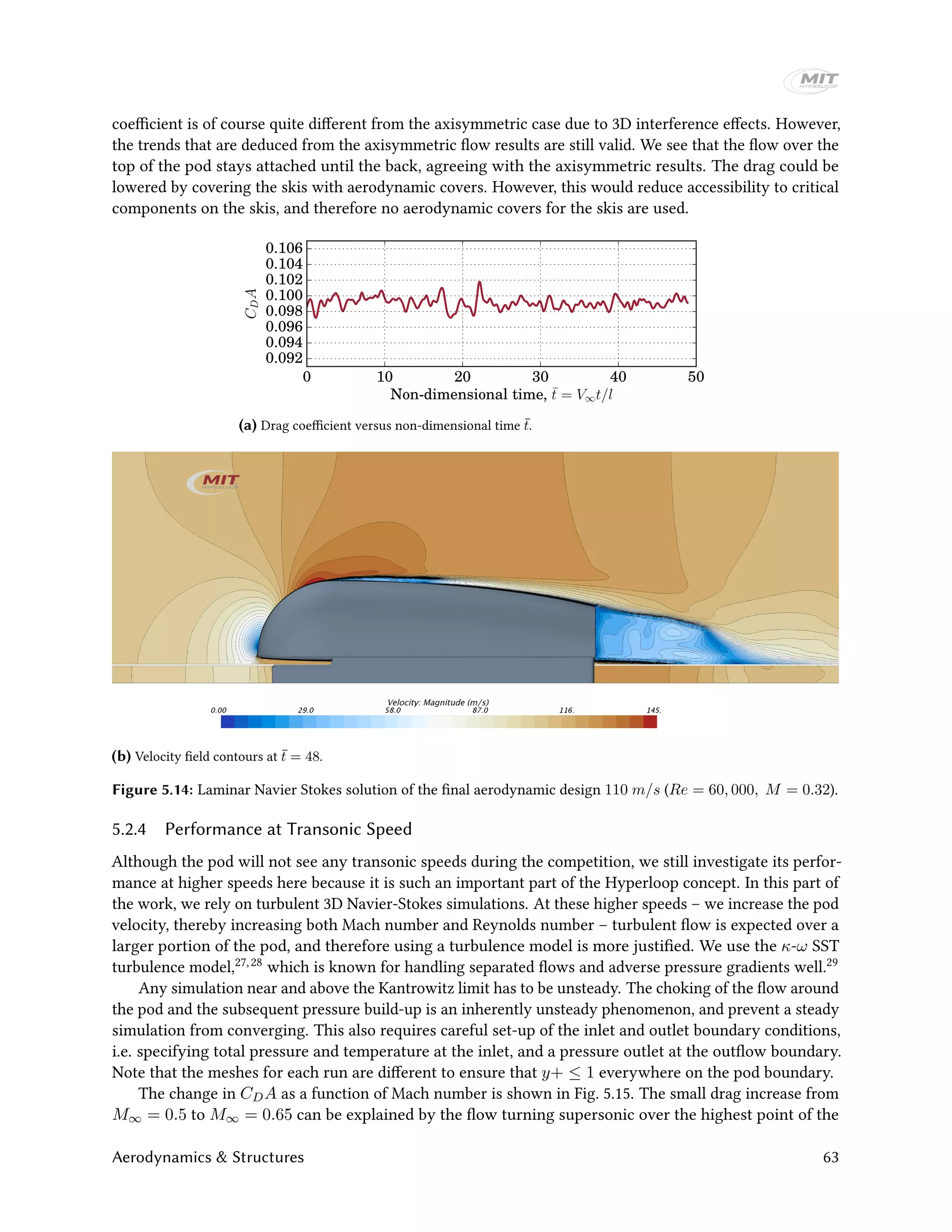
The results for the laminar Navier-Stokes simulations over the pod are shown in Fig. 5.14. We can see a
small degree of vortex shedding off the back of the pod, but the overall influence on the drag coefficient is
low, as shown in Fig. 5.14a. Vortex shedding is to be expected at these low Reynolds numbers.26 The drag
62 Final Report by MIT Hyperloop](https://image.slidesharecdn.com/mithyperloopfinalreport2017public-191204174448/75/Mit-hyperloop-final_report_2017_public-62-2048.jpg)
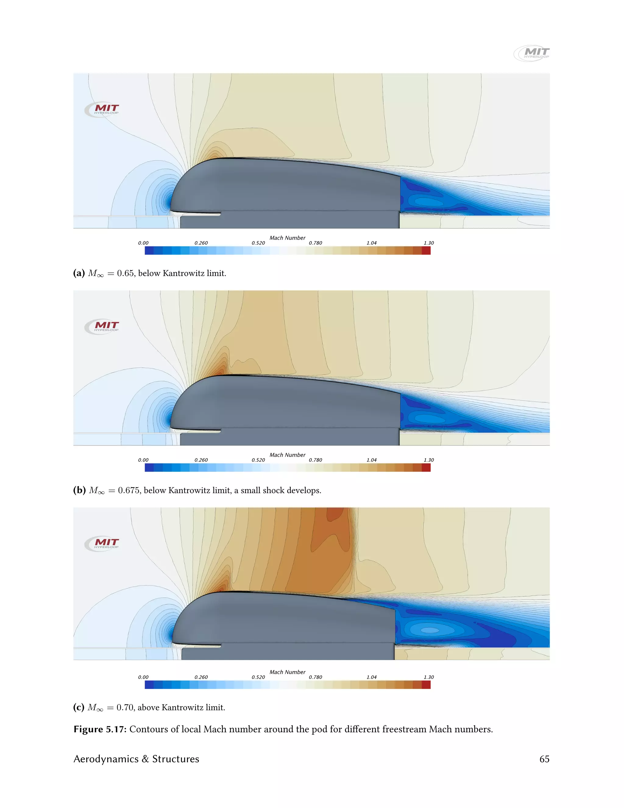
![pod (as shown in Fig. 5.17a), which results in a small shock with associated wave drag. Although part
of the flow over the pod is supersonic at those freestream Mach numbers, the flow has not choked yet,
because the supersonic region does not reach all the way to the tube boundaries. The flow around the pod
chokes around M∞ = 0.675, resulting in a large drag increase for larger Mach numbers. Due to the fact
that not all flow can continue past the pod, a pressure build-up in front of the pod results. Fig. 5.16 shows
the pressure coefficient along the tube, 1 m above the pod, which clearly shows a large pressure increase
in front of the pod for freestream Mach numbers higher than 0.675. The drag build-up due to exceeding
the Kantrowitz limit is signficant, the drag coefficient is three times as high for M∞ = 0.8 compared to
M∞ = 0.65. Note that part of the drag increase is also the result of the wave drag increase due to the
associated strong normal shock, as shown in Fig. 5.17c. Furthermore, the shock-induced boundary layer
separation for M∞ > 0.70 also increases the pressure drag.
The drag increase due to the exceeding the Kantrowitz limit is substantial: a three-fold increase in CDA
between M∞ = 0.65 and M∞ = 0.80. That additional drag increase results in a power loss of 31 kW.
However, it is questionable that a compressor used to avoid exceeding the Kantrowitz limit could compress
the air to feed it through the pod for less power. For example, the Hyperloop Alpha concept’s first stage
compressor has a power requirement of 276 kW,1 and Chin et al. found that for their configuration the
compressor power requirement exceeded 300 kW.5 For our configuration, if we assume an isentropic
efficiency for the compressor of 80% and a ductc area of 0.05 m2, the power requirement for the compressor
is 204 kW at M∞ = 0.80. Of course, if the power requirement for a compressor to avoid the Kantrowitz
limit is higher than the power loss due to the additional drag from exceeding the Kantrowitz limit, adding a
compressor would be futile.
0.45 0.50 0.55 0.60 0.65 0.70 0.75 0.80 0.85
Mach number, M∞
0.100
0.150
0.200
0.250
0.300
0.350
0.400
0.450
CDA
Figure 5.15: CDA as a function of Mach number for the final design. The large drag build-up starts around
M∞ = 0.675. Note that the freestream density is kept constant, therefore the Reynolds number increases pro-
portionally with Mach number.
-30 -20 -10 0 10 20 30
x [m]
-1.000
-0.500
0.000
0.500
PressureCoefficient,Cp
M∞ = 0.55
M∞ = 0.60
M∞ = 0.65
M∞ = 0.675
M∞ = 0.70
M∞ = 0.75
M∞ = 0.80
Figure 5.16: Pressure coefficient at 1 m above the base of the shell along tube for different Mach numbers.
c
The duct feeds the compressed air from the compressor outlet to the nozzle at the back of the pod.
64 Final Report by MIT Hyperloop](https://image.slidesharecdn.com/mithyperloopfinalreport2017public-191204174448/75/Mit-hyperloop-final_report_2017_public-64-2048.jpg)
![were alternated in between to increase in-plane shear stiffness desirable for load cases such as twisting
of the shell from asymmetric handling. As a result, a minimum QI sandwich structure that satisfies the
considerations above would entail a 2-core-2 [0/90 ± 45 core]S layup schedule. In terms of manufacturing,
a 2-core-2 laminate is also more amenable to infusion over a 1-core-1 due to the availability of open flow
channels along the fabric crimps, and thus allows better permeability for resin flow to minimize void
formation and dry spots.
For the shell areas that require fastening to the frame, a monolithic laminate is more attractive for the
higher compressive stiffness and resistance to hole edge delaminations. Therefore a 45◦ core pandown
was designed two inches from the bottom of the shell to form a reinforced lip region, with the 2-core-2
laminate transitioning to a 6-ply QI laminate. The outer and inner two plies of this lip region are continuous
with facesheets of the sandwich laminate to minimize delamination initiation on the surface of the layup
transition. Two 0◦/90◦ degree plies were inserted in the middle between the facesheets to form the
symmetric and balanced monolithic laminate throughout all bottom edges of the shell.
5.3.3 Structural Analysis
Micromechanical models were used to predict the carbon fiber/epoxy ply-level properties as inputs in a
finite element analysis of the shell structure under maximum load cases, such as ambient tube pressures in
the event of a preliminary test run. Microscale properties of the carbon fibers were first obtained through
manufacturing testing data, with Hexcel AS4 fibers having mean strengths of 4.6 GPa and stiffness of
231 GPa, and epoxy having a stiffness of 3.1 GPa. An estimate of 40% fiber volume fracture was used,
which is typical of woven aerospace laminates. By knowing the density of the fibers, a 197 gsm Hexcel AS4
fabric was estimated to have longitudinal and transverse stiffness of 48 GPa (plain weave with same warp
and weft fibers).
The shell’s structural properties are analyzed using Abaqus. The CFD results are used to get the correct
loads on the structure. The shell is analyzed for the structural design case (full speed – 250 mph at 1/10th
of an atmosphere – 10133 Pa) and for a handling case, where the shell is pulled up from its six suspension
points.
The success criteria for the structural design was defined here to limit deformation to 1 mm as is
consistent with the anticipated clearance between the inner lip of the shell and the bottom closeout, and to
ensure no failure at the bolt location. For the 1/10 atmosphere structural design case results in concentrated
stresses close to the first holes towards the front of the vehicle with a peak stress of 14 MPa. However,
these values are significantly lower than the anticipated failure strength, even with a large factor of safety of
2. If we assume locally only the half of the fibers are engaged in the direction for failure, then an allowable
stress of 1/2 986.2 (unidirectional strength) = 493 MPa for the CFRP can be estimated. The Margin of
Safety (MS) is then,
MS =
σallowable
σlimit · SF
− 1 =
493
2 · 14
− 1 = 17.
It is also important to note that even if a B-basis allowable (generally in the range of 80% of the mean
strength value depending on scatter) was used here, the MS would still be 13, and thus we do not anticipate
failure for the shell under 1/10th atmospheric loading at top speed.
The maximum deflection of 0.5 mm at the nose of the shell is also well within the 1 mm limit as
outlined before, and thus the structural design fulfills the intended bounding operating load case.
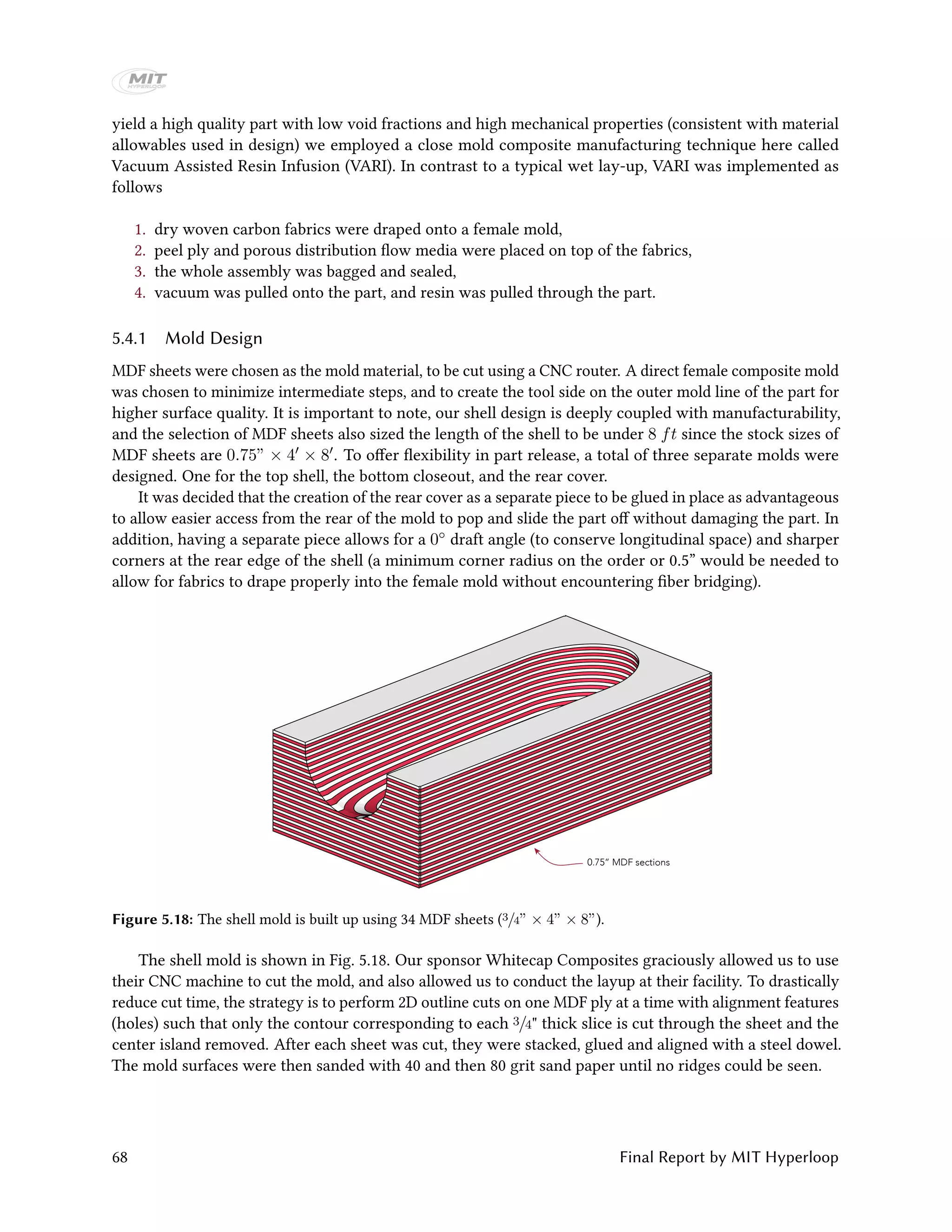
5.4 Shell Manufacturing
Manufacturing the shell also posed some key challenges, most notably the two month build time constraint
and a lack of access to an autoclave system. Therefore, an out-of-autoclave process was utilized. To
Aerodynamics & Structures 67](https://image.slidesharecdn.com/mithyperloopfinalreport2017public-191204174448/75/Mit-hyperloop-final_report_2017_public-67-2048.jpg)
![20
25
30
35
40
45
0 100 200 300 400 500 600 700
Temperature[C]
Time [s]
Cell #1 9A discharge (Room condition)
Cell #2 9A discharge (Room condition)
Cell #1 9A discharge (3000 Pascal)
Cell #2 9A discharge (3000 Pascal)
Figure 6.11: Temperature of cells during discharge in vacuum chamber.
6.2.2 Brakes Electronics
The electrical system of the brakes consists of five parts: 24V proportional valve, 24V on/off valve, a 24V
pump motor, a 24V pressure sensor and two 24V linear potentiometers, as shown in Fig. 6.12. For more
information on the sensors, please refer to Section 6.1.5.
Proportional Valve
Linear potentiometer
Brake/Low
speed PCB
(PID control)
Pressure transducer
Bang-bang valve
Motor
Linear potentiometer
● +24 V
● GND
● 4 - 20mA analog output
Pressure transducer
● +24 V
● GND
● 4 - 20mA analog output
● (M12 connector)
Bang-bang valve
● Coil + (open needs +24 V, 22 W)
● Coil - (can be connected to GND)
● GND
● Speed analog control
● Forward/reverse digital signal
36V
battery
Proportional Valve
● +24 V (3 Amps)
● GND
● 0 - 5 V analog input (can select 4 - 20 mA, 0 - 10 V)
Figure 6.12: Brakes electronics system overview.
The valves and motors all have built in controllers, thus we care mainly about powering them and
interfacing them with the Brake/Lowspeed PCB. This is realized by the brake interface PCB. One should
note that the interfaces of the enable signals for the low speed motors and actuators are also realized on
this PCB.
80 Final Report by MIT Hyperloop](https://image.slidesharecdn.com/mithyperloopfinalreport2017public-191204174448/75/Mit-hyperloop-final_report_2017_public-80-2048.jpg)
![-3 -2 -1 0 1 2 3
0
0.5
1
1.5
2
2.5
3
(a) Response times
-3 -2 -1 0 1 2 3
0
0.05
0.1
0.15
0.2
(b) Overshoots
Figure 7.6: Step response behavior of the brake hydraulic controller, across a spectrum of requested brake posi-
tion step sizes. Each point indicates a random brake position setpoint (evenly distributed between fully open and
fully closed) issued to the brake controller, plotted by the change in position setpoint from the last command. Step
commands are in inches, with positive numbers indicating commands to open, and negative numbers indicating
commands to close. Response time indicates the time it took the controller to first get to within 0.1 inches of the
setpoint. Overshoots indicates the farthest past the setpoint the brakes went during the control window.
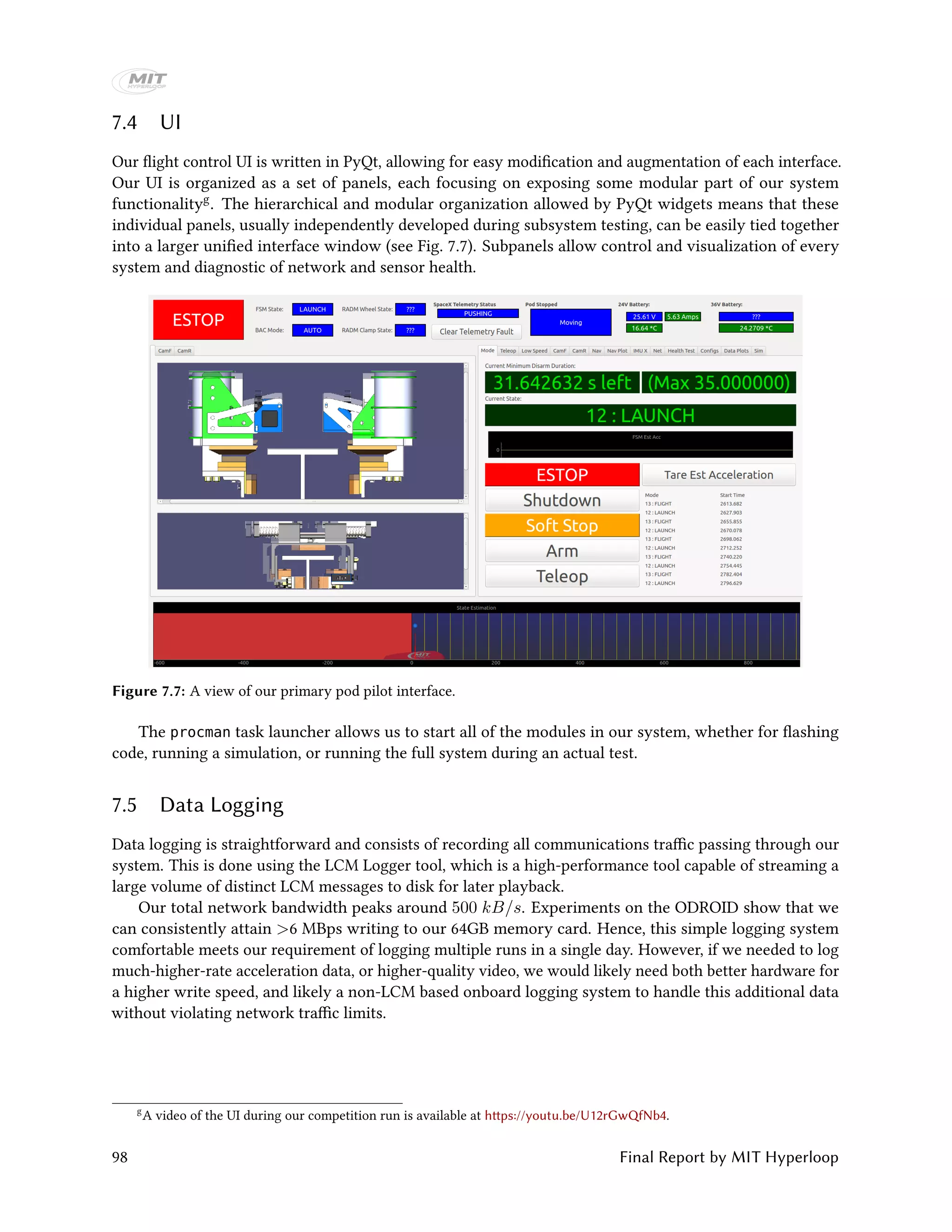
(VectorNav VN-100s mounted on the pod body, above the suspension) with fiducial stripe detections from a
high-rate optical color detector. The IMUs are integrated to continuously produce estimated velocities and
positions, while the strips are leveraged to periodically correct accumulated drift.
Specifically, we consider the state to be xk = {qk, ˙qk, ¨qk}, for position along the tube qk at time step
k, and a covariance estimate of the state Σk, summarized in a Gaussian distribution γstate
k = {xk, Σk}.
Between fiducial strip detections, we iteratively update the state estimate with a standard EKF process
update.31 We use a first-order double-integrator process model
xk = xk−1 + δt[ ˙qk−1, ¨qk−1, 0]T
.
IMU measurements, alongside a pod stopping detector, provide direct observations of ¨q and ˙q respectively.
e
SpaceX furnished the tube with a 4" wide retroreflective orange strip every 100’ on the inside of the tube; see Section 6.1.2
for details.
96 Final Report by MIT Hyperloop](https://image.slidesharecdn.com/mithyperloopfinalreport2017public-191204174448/75/Mit-hyperloop-final_report_2017_public-96-2048.jpg)

![0
15
50
6010
100
40
150
5 20
0 0
(a) Lift force
0
15
20
6010
40
40
60
5 20
0 0
(b) Drag force
Figure 8.5: Experimental results from the rotary test rig for the LCM configuration.
0
10
20
30
40
50
60
70
80
90
0 10 20 30 40 50
Force [N]
Speed [m/s]
Drag #1
Li3 #1
Drag #2
Li3 #2
Drag #3
Li3 #3
Drag #4
Li3 #4
Figure 8.6: Repeatability between runs of rotary test rig.
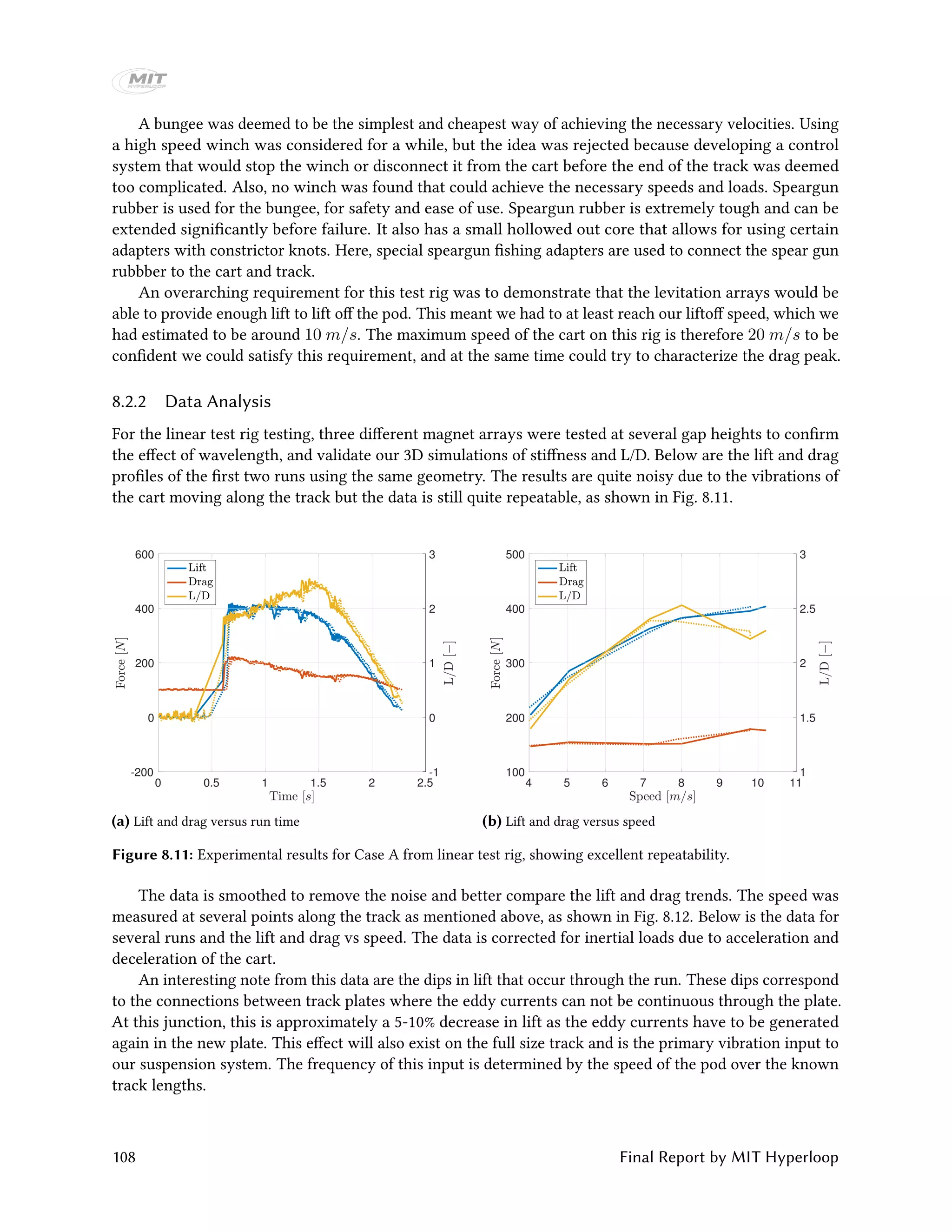
8.2 Linear Test Rig
Besides testing the LCM and brake arrays, it was desired to also test the levitation arrays. The primary goal
was to design a rig that could be used to test an array that was identical in configuration and as close as
possible in size to the full-scale array, such as to minimize any uncertainty about the performance of our
levitation skis, while corroborating our simulation data.
8.2.1 Design
To keep the configuration as close as possible to our full ski array design we decided the nominal test array
would have the same thickness (3/4”) , width (2”), gap height (10 mm), magnet grade (N42), and number
of periods (2) as the final ski design. Furthermore, the aluminium plate on which the configuration was
riding had to be the correct alloy (6101-T6) and have the same thickness (1⁄2”) as the actual track. Note that
at the initial time of design the thickness and width values of the array were slightly different (1/2"" and 4”,
respectively) but this did not dramatically affect the design of the rig.
Levitation Testing Campaign 105](https://image.slidesharecdn.com/mithyperloopfinalreport2017public-191204174448/75/Mit-hyperloop-final_report_2017_public-105-2048.jpg)
![Figure 8.7: Comparison between stiffness of LCM configuration as found from experimental and simulation
results.
0
10
20
30
40
50
60
70
80
0 10 20 30 40 50
Force [N]
Speed [m/s]
Experimental Drag
Experimental Li9
Simulated Drag
Simulated Li9
Figure 8.8: Comparison of experimental and simulation data for LCM configuration at 10 mm offset, as measured
using the rotary test rig.
A rotary test rig was considered for the levitation array testing as well, again considering a “record
player" and “edge riding" configuration. The edge riding configuration was dimissed for the same reasons
as before. However, because the levitation arrays are larger than the LCM and brake arrays, also the record
player configuration is problematic. For the levitation arrays the speed variation across the tranverse
direction of the array for a reasonably sized plate would be too high. Furthermore, it would be prohibitively
expensive to obtain an Al 6101-T6 plate large enough to make such a disc out of.
A test rig where the array is stationary but the aluminum plate shoots under it, was also considered.
For cost and safety reasons, this idea was not further pursued.
This left a linear test rig where the a magnet array moves relative to a stationary track. Given the short
time frame, the linear test rig was designed with ease of manufacturing in mind. A description of the design
of the linear test rig is provided below.
The track is shown in Fig. 8.9. As shown, only part of the track has Al 6101 I-beams on it, which kept
the cost of the rig down because we only intended to measure at relatively high speeds. The total track is
75 ft long. A simple simulation of the cart dynamics showed that a 20 m long track would be sufficient to
106 Final Report by MIT Hyperloop](https://image.slidesharecdn.com/mithyperloopfinalreport2017public-191204174448/75/Mit-hyperloop-final_report_2017_public-106-2048.jpg)
![0 0.5 1 1.5 2 2.5
-200
0
200
400
600
800
-1
0
1
2
3
4
(a) Lift and drag versus run time
6 7 8 9 10 11 12 13
200
300
400
500
600
700
2
2.2
2.4
2.6
2.8
3
(b) Lift and drag versus speed
Figure 8.12: Experimental results for Case E from linear test rig.
We show a comparison between numerical and experimental results for several runs in Table 8.1 and
Fig. 8.13. The numerical results are quite close to the experimental results, giving additional confidence to
the levitation design which was based off of the numerical results.
Table 8.1: Comparison of experimental results with numerical results for linear test rig
Magnet configuration Simulation data Simulation data
at 10 m/s at peak speed
Array Array Array # periods Gap height] Lift Drag L/D Lift Drag L/D
length [in] width [in] thickness [in] [−] [mm] [N] [N] [−] [N] [N] [−]
A 16 2 1/2 2 12 426 243 1.8 400 210 1.9
B 16 2 3/4 2 12 n/a n/a n/a 680 290 2.3
C 16 2 3/4 2 9 n/a n/a n/a 850 310 2.7
D 16 2 3/4 2 6 1242 604 2.1 1100 390 2.8
E 16 2 3/4 1 6 700 310 2.3 720 260 2.8
F 16 2 3/4 1 9 600 250 2.4 550 250 2.2
G 16 2 3/4 1 12 500 200 2.5 450 220 2.0
0
100
200
300
400
500
600
700
800
Case A Case E Case F Case G
Force [N]
Simula8on Li<
Tes8ng Li<
Simula8on Drag
Tes8ng Drag
Figure 8.13: Comparison of numerical and experimental results for linear test rig.
Levitation Testing Campaign 109](https://image.slidesharecdn.com/mithyperloopfinalreport2017public-191204174448/75/Mit-hyperloop-final_report_2017_public-109-2048.jpg)