Download to read offline
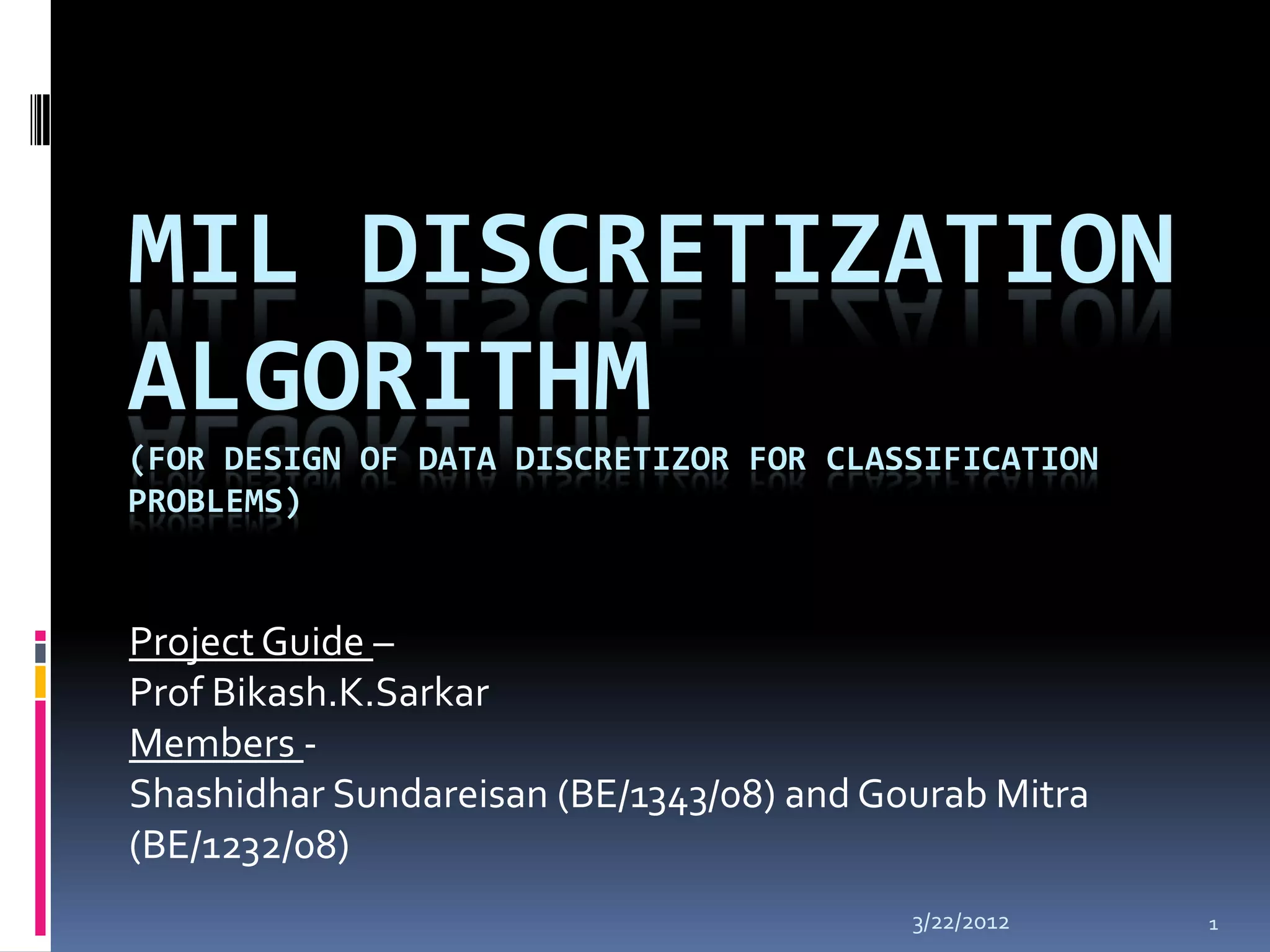


![ In the first interval, Tot_CTS < TS/3 . So, we
merge it with the next interval.
Update Tot_CTS= Tot_CTS + CTS[1] (= 3 + 3)
Update TS = TS + m/n (= 12 + 12)
3/22/2012 7](https://image.slidesharecdn.com/milppt14nov-120322150104-phpapp02/75/Minimum-Information-Loss-Algorithm-7-2048.jpg)

![ Still, Tot_CTS < TS/3. So, we merge again.
Update Tot_CTS= Tot_CTS + CTS[1] (= 6 + 8)
Update TS = TS + m/n (= 24 + 12)
3/22/2012 9](https://image.slidesharecdn.com/milppt14nov-120322150104-phpapp02/75/Minimum-Information-Loss-Algorithm-9-2048.jpg)


![20
18
16
14
12
Frequency
10
8 Optimal Merged Sub-
6 interval
4
2
0
CTS[0]CTS[1]CTS[2]CTS[3]CTS[4]CTS[5]CTS[6]
3/22/2012 15](https://image.slidesharecdn.com/milppt14nov-120322150104-phpapp02/75/Minimum-Information-Loss-Algorithm-15-2048.jpg)
![Final Frequency Chart
45
40
35
30
25 Frequency
20
Optimal Merged Sub-
15 interval
10
5
0
CTS[0] CTS[1] CTS[2] CTS[3] CTS[4]
3/22/2012 16](https://image.slidesharecdn.com/milppt14nov-120322150104-phpapp02/75/Minimum-Information-Loss-Algorithm-16-2048.jpg)


This document describes the MIL (Multiple Intervals List) algorithm for discretization of continuous attributes for classification problems. It involves 4 scans of the training data: 1) calculate min and max, 2) calculate thresholds, 3) calculate optimal merged sub-intervals, 4) discretize attributes. An example shows applying it to a CGPA attribute to classify students into grade categories. The algorithm merges sub-intervals until their combined instances exceed 1/3 of the threshold. It has linear time complexity and requires only 4 data scans, making it efficient compared to other discretization methods.


