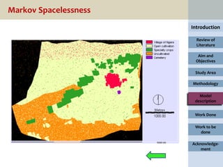
This document provides an overview of the methodology used to model and analyze watershed dynamics using cellular automata and Markov chain analysis. The key steps include:
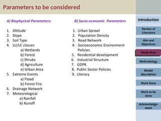
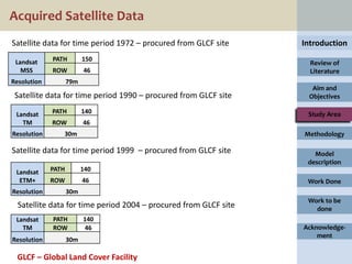
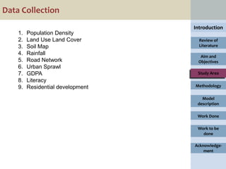
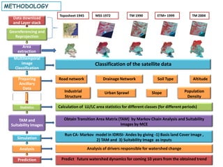
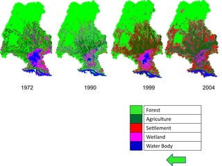
1. Classifying satellite images from multiple time periods to generate land use/land cover databases.
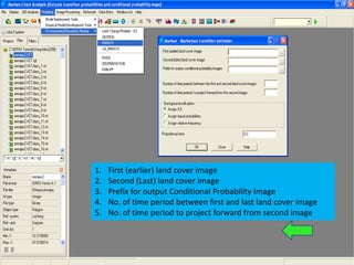
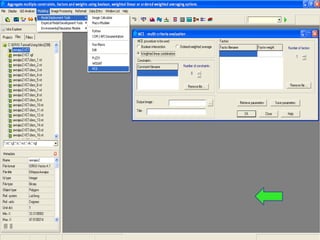
2. Deriving transition area matrices and suitability images based on the classifications using Markov chain analysis and multi-criteria evaluation.
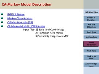
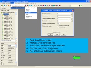
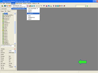
3. Running a cellular automata-Markov model in IDRISI software using the land cover database, transition matrices, and suitability images to simulate watershed changes.
4. Analyzing the key drivers of watershed changes and predicting future watershed dynamics over the next 10 years based on observed trends.