Economics and importance, display implement encourage bahahaia hwg igwii igwbwjiwkw hgwhiabwva nhgtiwo kgfvwvwj bhagay bhwjwjwiwbwg jhwbwh khegwh jwgvwhhwhw Hakhha good.

1. MICROECONOMICS
LECTURE 18
Lecture 09
1

2. MICROECONOMICS
THEORY OF CONSUMER CHOICE PART -II
Dr. Khurram Iftikhar

3. 11.2 MARGINAL UTILITY THEORY
Maximizing Total Utility
The goal of a consumer is to allocate the available
budget in a way that maximizes total utility.
The consumer achieves this goal by choosing the point
on the budget line at which the sum of the utilities
obtained from all goods is as large as possible.

4. 11.2 MARGINAL UTILITY THEORY
This outcome occurs when a person follows the utility-
maximizing rule:
1. Allocate the entire available budget.
2. Make the marginal utility per dollar spent the same
for all goods.

5. 11.2 MARGINAL UTILITY THEORY
Allocate the Available Budget
The available budget is the amount available after
choosing how much to save and how much to spend on
other items.
The saving decision and all other spending decisions
are based on the same utility maximizing rule that you
are learning here and applying to Tina’s decision about
how to allocate a given budget to water and gum.

6. 11.2 MARGINAL UTILITY THEORY
Equalize the Marginal Utility Per Dollar Spent
Spending the entire available budget doesn’t
automatically maximize utility.
Dollars might be misallocated—spend in ways that don’t
maximize utility.
Making the marginal utility per dollar spent the same for
all goods gets the most out of a budget.

7. 11.2 MARGINAL UTILITY THEORY
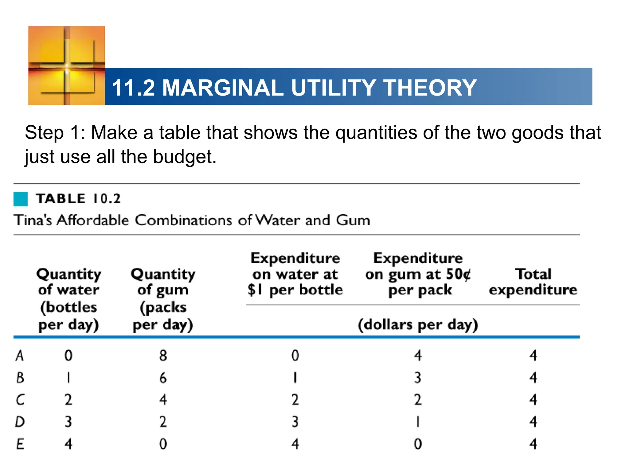
Step 1: Make a table that shows the quantities of the two goods that
just use all the budget.

8. 11.2 MARGINAL UTILITY THEORY
Step 2: Calculate the marginal utility per dollar spent on the
two goods.
Marginal utility per dollar spent
The increase in total utility that comes from the last
dollar spent on a good.

9. 11.2 MARGINAL UTILITY THEORY
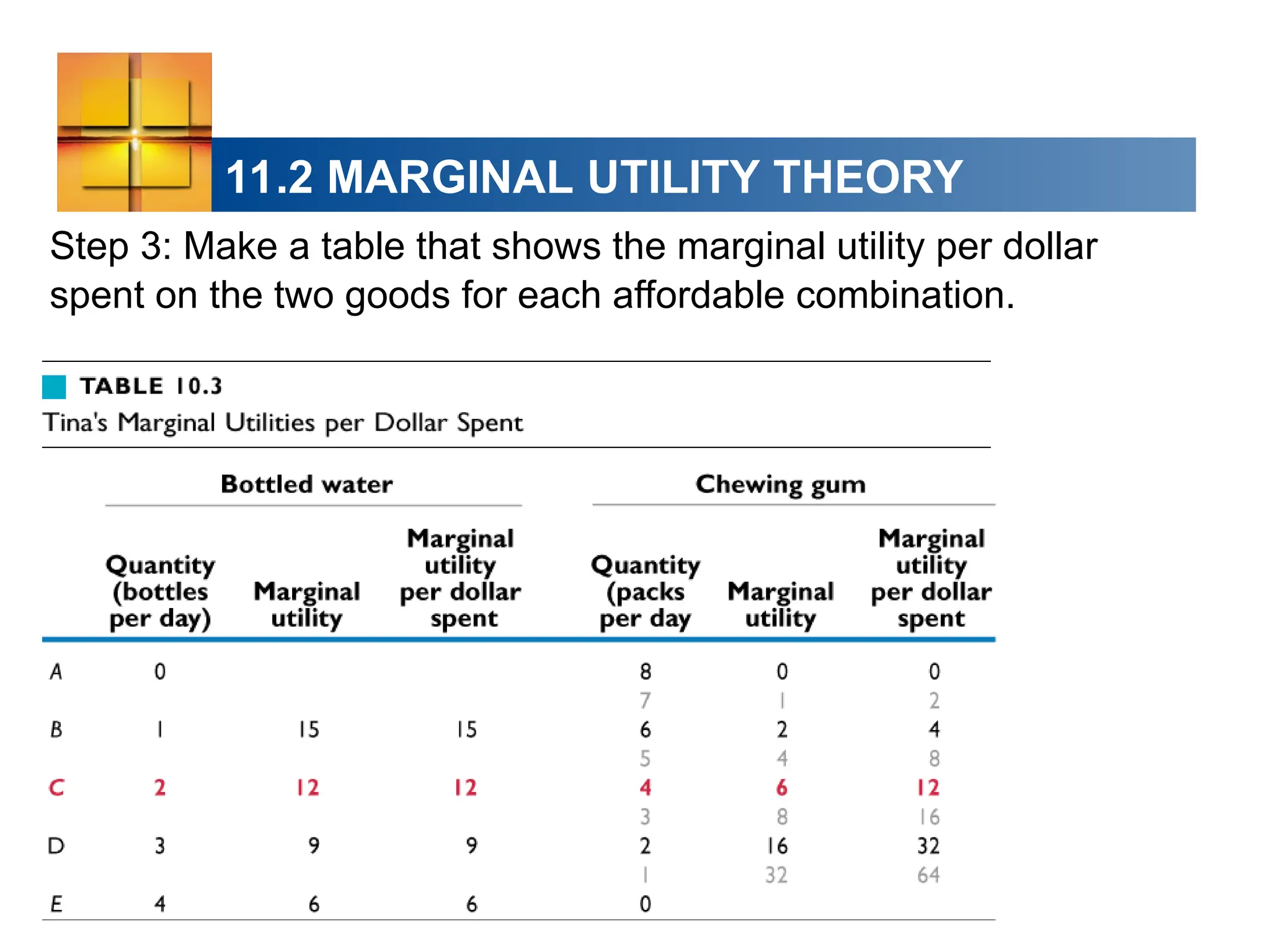
Step 3: Make a table that shows the marginal utility per dollar
spent on the two goods for each affordable combination.

10. 11.2 MARGINAL UTILITY THEORY
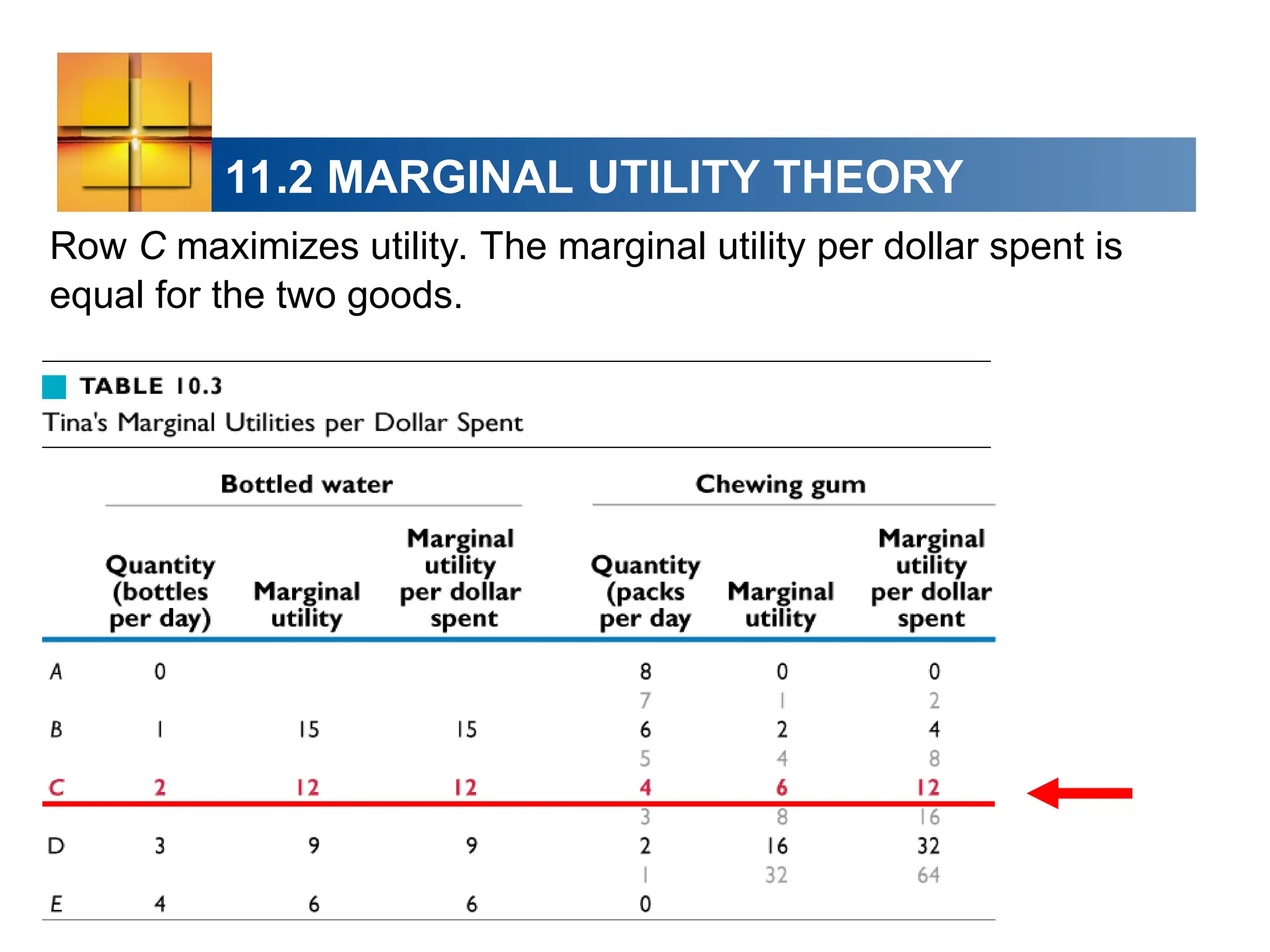
Row C maximizes utility. The marginal utility per dollar spent is
equal for the two goods.

11. 11.2 MARGINAL UTILITY THEORY
Units of Utility
In calculating Tina’s utility-maximizing choice in Table
11.3, we have not used the concept of total utility.
All our calculations use marginal utility and price.
Changing the units of utility doesn’t affect our prediction
about the consumption choice that maximizes total
utility.

12. 11.2 MARGINAL UTILITY THEORY
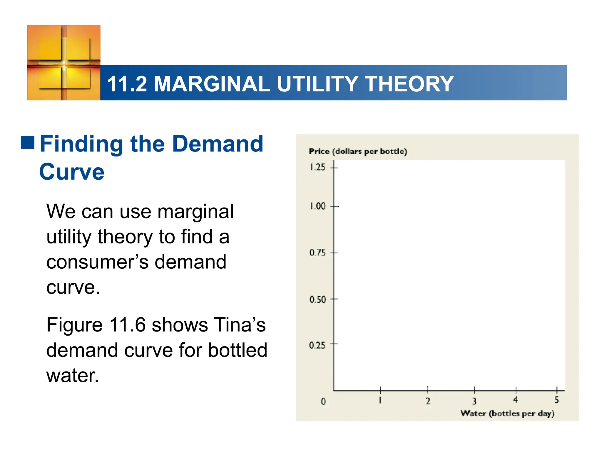
Finding the Demand
Curve
We can use marginal
utility theory to find a
consumer’s demand
curve.
Figure 11.6 shows Tina’s
demand curve for bottled
water.

13. 11.2 MARGINAL UTILITY THEORY
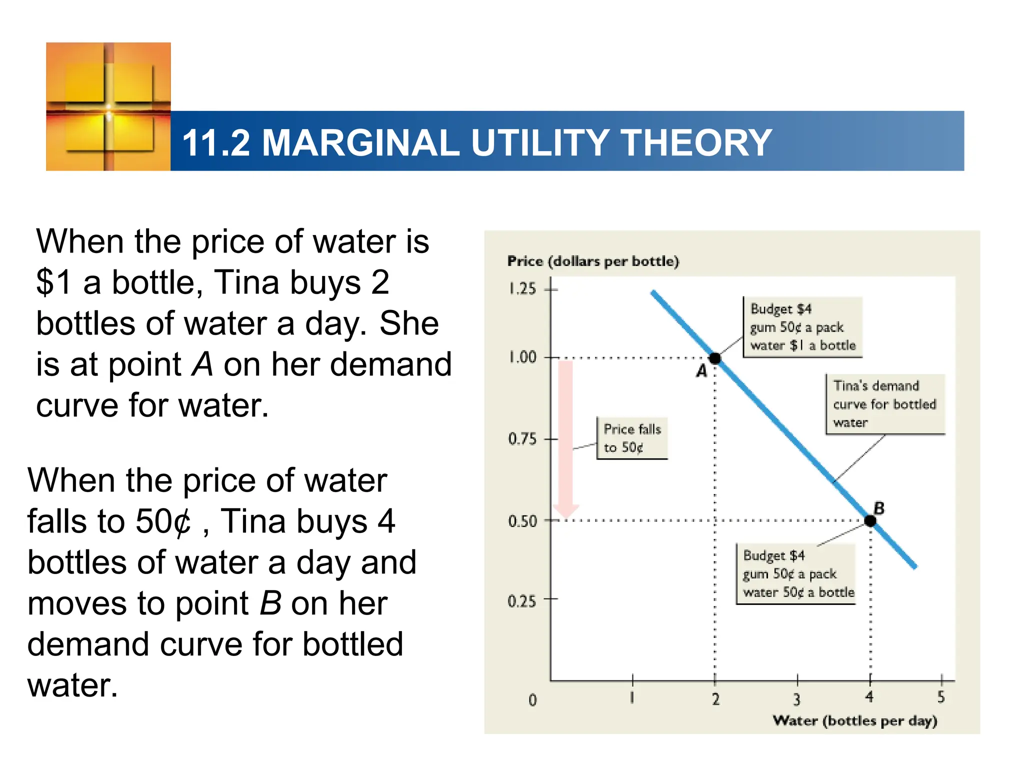
When the price of water is
$1 a bottle, Tina buys 2
bottles of water a day. She
is at point A on her demand
curve for water.
When the price of water
falls to 50¢ , Tina buys 4
bottles of water a day and
moves to point B on her
demand curve for bottled
water.

14. 11.2 MARGINAL UTILITY THEORY
Marginal Utility and the Elasticity of Demand
If, as the quantity consumed of a good increases,
marginal utility decreases quickly, the demand for the
good is inelastic.
The reason is that for a given change in the price, only
a small change in the quantity consumed of the good is
needed to bring its marginal utility per dollar spent back
to equality with that on all the other items in the
consumer’s budget.

15. 11.2 MARGINAL UTILITY THEORY
But if, as the quantity consumed of a good increases,
marginal utility decreases slowly, the demand for that
good is elastic.
In this case, for a given change in the price, a large
change in the quantity consumed of the good is needed
to bring its marginal utility per dollar spent back to
equality with that on all the other items in the
consumer’s budget.

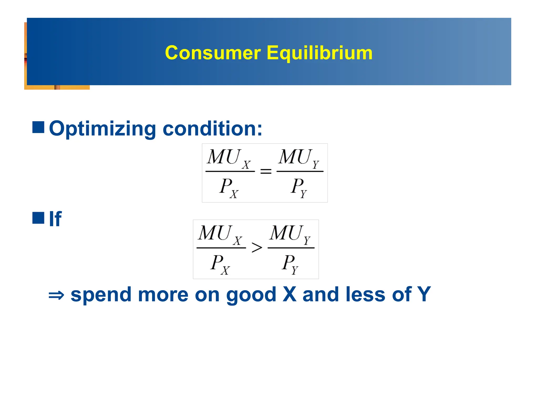
16. Consumer Equilibrium
So far, we have assumed that any amount of
goods and services are always available for
consumption
In reality, consumers face constraints
(income and prices):
Limited consumers income or budget
Goods can be obtained at a price

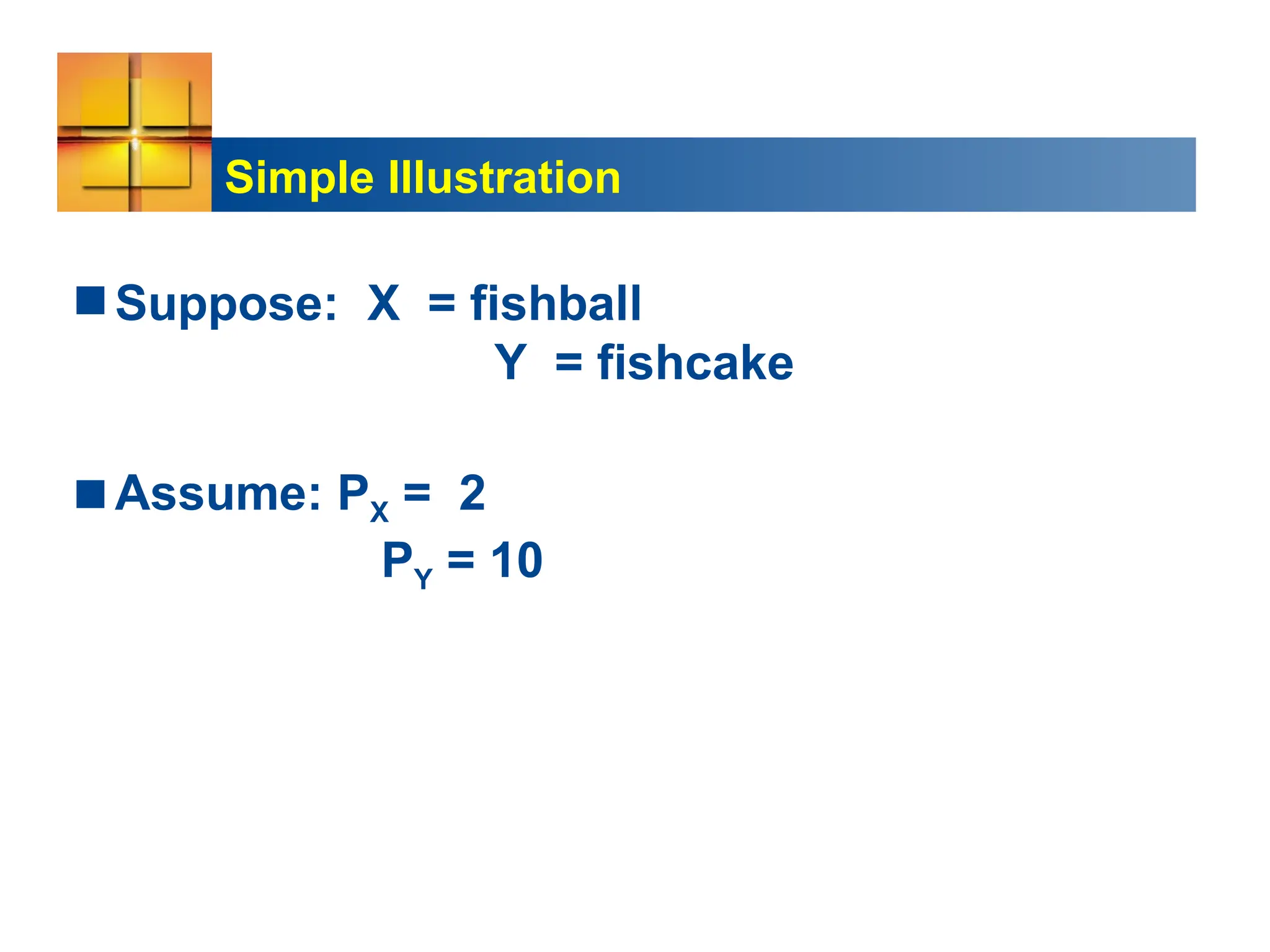
17. Some simplifying assumptions
Consumer’s objective: to maximize his/her
utility subject to income constraint
2 goods (X, Y)
Prices Px, Py are fixed
Consumer’s income (I) is given

18. Consumer Equilibrium
Marginal utility per price  additional utility
derived from spending the next price on the
good
MU per Price = MU
P

19. Consumer Equilibrium
Optimizing condition:
If
 spend more on good X and less of Y

20. Simple Illustration
Suppose: X = fishball
Y = fishcake
Assume: PX = 2
PY = 10

21. Numerical Illustration
Qx
TUX
MUX
MUx
Px
QY
TUY
MUY
MUy
Py
1 30 30 15 1 50 50 5
2 39 9 4.5 2 105 55 5.5
3 45 6 3 3 148 43 4.3
4 50 5 2.5 4 178 30 3
5 54 4 2 5 198 20 2
6 56 2 1 6 213 15 1.5

22. Cont.
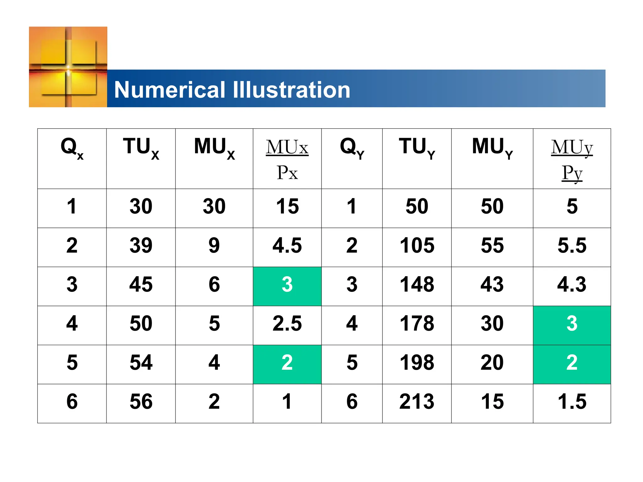
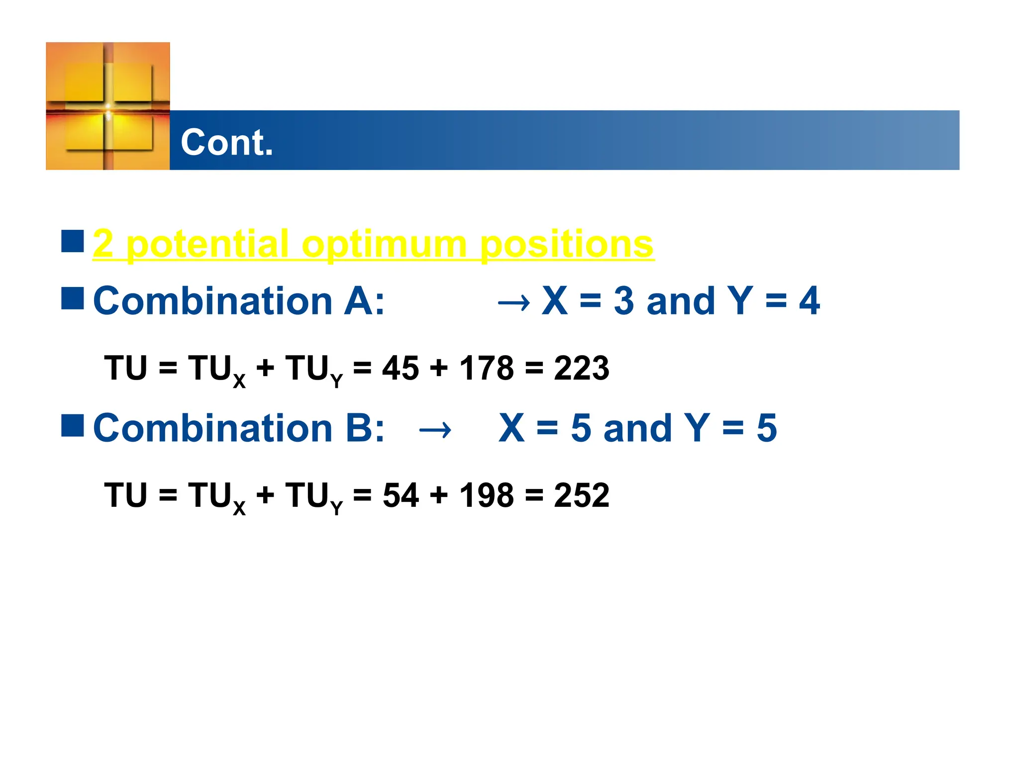
2 potential optimum positions
Combination A:  X = 3 and Y = 4
TU = TUX + TUY = 45 + 178 = 223
Combination B:  X = 5 and Y = 5
TU = TUX + TUY = 54 + 198 = 252

23. Cont.
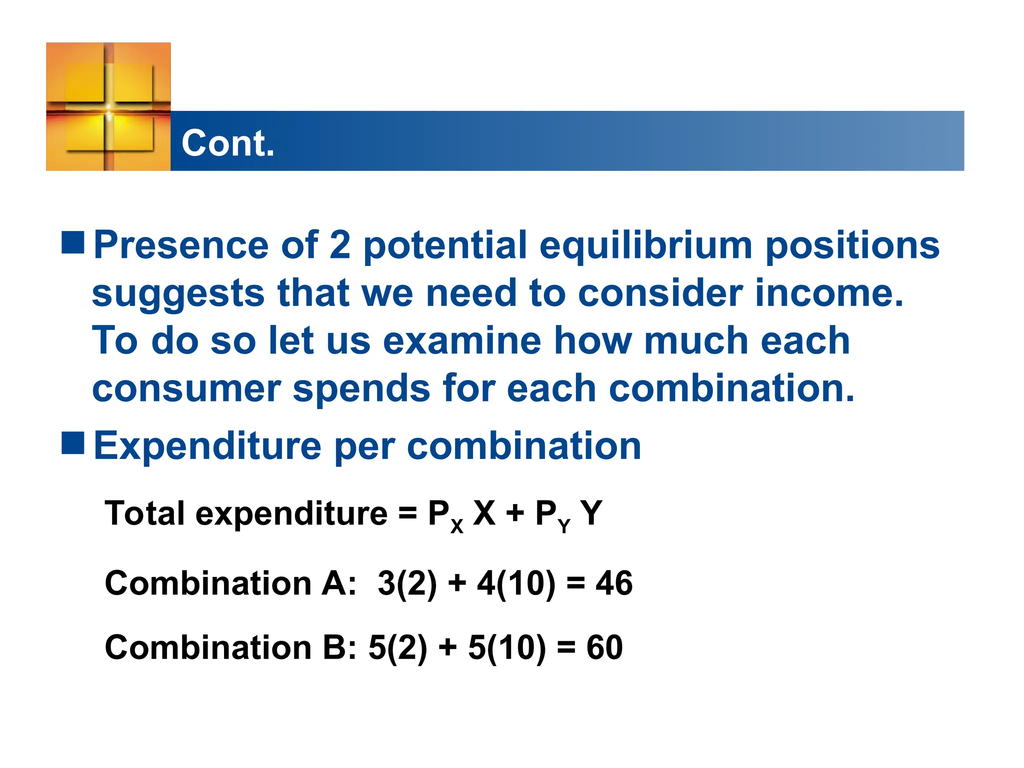
Presence of 2 potential equilibrium positions
suggests that we need to consider income.
To do so let us examine how much each
consumer spends for each combination.
Expenditure per combination
Total expenditure = PX X + PY Y
Combination A: 3(2) + 4(10) = 46
Combination B: 5(2) + 5(10) = 60

24. Cont.
Scenarios:
If consumer’s income = 46, then the optimum is
given by combination A. .…Combination B is not
affordable
If the consumer’s income = 60, then the optimum is
given by Combination B….Combination A is
affordable but it yields a lower level of utility