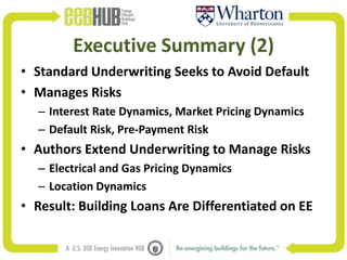
The document summarizes a paper that proposes a new method for commercial mortgage lenders to explicitly factor energy risk and building energy efficiency into mortgage underwriting. It finds that standard underwriting does not account for risks from volatile energy prices, which can significantly impact building cash flows. The authors develop a model to simulate cash flows under different energy price scenarios and incorporate these risks into loan valuations. The results show loan valuations are 8.5% lower when accounting for energy, with larger reductions for larger buildings and loans. The paper concludes this method can help lenders more accurately price loans based on location-specific energy risks and efficiency levels.

1. Energy Efficiency And
Commercial-Mortgage Valuation
Paper Written By
Dwight Jaffee, Richard Stanton and Nancy Wallace
http://www.law.berkeley.edu/files/bclbe/DOE_Valuation_9.25.12.pdf
January 17, 2012
Presentation by Matthew Kwatinetz1 EEB HUB
Moderated and Discussed by Scott Muldavin
1Mr. Kwatinetz is presenting this paper in absence of the authors. Every effort has
been made to accurately convey the intention and conclusion of the authors. Any
errors, omissions are Mr. Kwatinetz’ alone and do not reflect the work of the authors.

2. Executive Summary (1)
• Commercial Office Buildings Are Intense Users of Energy
• Building Energy Intensity Creates Different Cost Structure
– For Landlord and/or Tenant
• Energy Prices are Volatile
• Non-EE Buildings Are More Exposed to Volatility
– Have more loan default risk
– Are more expensive per square foot (SF)
– Should be less attractive to investors and have different loan
terms
• Yet Existing Loan Practices Provide No Incentive for EE
• This Paper Proposes a Method for Lenders Explicitly
Taking Energy Risk (and level of EE) into Mortgage
Underwriting

3. Executive Summary (2)
• Standard Underwriting Seeks to Avoid Default
• Manages Risks
– Interest Rate Dynamics, Market Pricing Dynamics
– Default Risk, Pre-Payment Risk
• Authors Extend Underwriting to Manage Risks
– Electrical and Gas Pricing Dynamics
– Location Dynamics
• Result: Building Loans Are Differentiated on EE

4. Traditional Mortgage
Underwriting

5. Traditional Mortgage Underwriting
Primary Goal: Avoid Default
• Risk Management
– Interest Rates, Market Pricing/Rents
– Default, Pre-Payment
• Variables
– Principle, Rate, Maturity, Amortization Schedule
• Metrics
– Loan to Value (LTV): Sized by Market/Risk (65%)
– Debt Service Coverage Ratio (DSCR): How much does
annual net income (NOI) cover annual amortized
debt service payment? (1.25)

6. Underwriting: Cash Flows
Year 1 Year 2 Year 3 Year 4 Year 5
Gross potential revenue $408,000 $416,160 $424,483 $432,973 $441,632
Revenue Growth Estimate 2.0% 2.0% 2.0% 2.0% 2.0%
Vacancy 5.0% 5.0% 5.0% 5.0% 5.0%
Rental Value of Vacancy $20,400 $20,808 $21,224 $21,649 $22,082
Subtotal GROSS POTENTIAL REVENUE $387,600 $395,352 $403,259 $411,324 $419,551
Collection Loss & Concessions $27,132 $27,675 $28,228 $28,793 $29,369
Management Fee $17,054 $17,395 $17,743 $18,098 $18,460
Net Rental Income $324,034 $330,514 $337,125 $343,867 $350,744
Expense Recovery $116,280 $60,489 $61,699 $62,933 $64,191
Effective Gross Income (EGI) $440,314 $391,003 $398,823 $406,800 $414,936
Operating Expenses $116,280 $120,978 $123,397 $125,865 $128,383
Net Operating Income (NOI) $324,034 $270,025 $275,426 $280,934 $286,553

7. Underwriting: NNN (Triple Net)
Year 1 Year 2 Year 3 Year 4 Year 5
Gross potential revenue $408,000 $416,160 $424,483 $432,973 $441,632
Revenue Growth Estimate 2.0% 2.0% 2.0% 2.0% 2.0%
Vacancy 5.0% 5.0% 5.0% 5.0% 5.0%
Rental Value of Vacancy $20,400 $20,808 $21,224 $21,649 $22,082
Subtotal GROSS POTENTIAL REVENUE $387,600 $395,352 $403,259 $411,324 $419,551
Collection Loss & Concessions $27,132 $27,675 $28,228 $28,793 $29,369
Management Fee $17,054 $17,395 $17,743 $18,098 $18,460
Net Rental Income $324,034 $330,514 $337,125 $343,867 $350,744
Expense Recovery $116,280 $60,489 $61,699 $62,933 $64,191
Effective Gross Income (EGI) $440,314 $391,003 $398,823 $406,800 $414,936
Operating Expenses $116,280 $120,978 $123,397 $125,865 $128,383
Net Operating Income (NOI) $324,034 $270,025 $275,426 $280,934 $286,553

8. Underwriting NNN: DSCR
Year 1 Year 2 Year 3 Year 4 Year 5
Net Rental Income $324,034 $330,514 $337,125 $343,867 $350,744
Expense Recovery $116,280 $120,978 $123,397 $125,865 $128,383
Effective Gross Income (EGI) $440,314 $451,492 $460,522 $469,732 $479,127
Operating Expenses $116,280 $120,978 $123,397 $125,865 $128,383
Net Operating Income (NOI) $324,034 $330,514 $337,125 $343,867 $350,744
Debt Service Payment ($116,280) ($116,280) ($116,280) ($116,280) ($116,280)
Debt Service Coverage Ratio (DSCR) 1.24 1.26 1.29 1.31 1.34
Cash Flow After Debt Service $61,822 $68,302 $74,913 $81,655 $88,532

9. Underwriting NNN: Expenses External
Year 1 Year 2 Year 3 Year 4 Year 5
Net Rental Income $324,034 $330,514 $337,125 $343,867 $350,744
Expense Recovery $116,280 $120,978 $123,397 $125,865 $128,383
Effective Gross Income (EGI) $440,314 $451,492 $460,522 $469,732 $479,127
Operating Expenses $116,280 $120,978 $123,397 $125,865 $128,383
Net Operating Income (NOI) $324,034 $330,514 $337,125 $343,867 $350,744
Debt Service Payment ($116,280) ($116,280) ($116,280) ($116,280) ($116,280)
Debt Service Coverage Ratio (DSCR) 1.24 1.26 1.29 1.31 1.34
Cash Flow After Debt Service $61,822 $68,302 $74,913 $81,655 $88,532

10. Traditional Underwriting Risks
• Uncertainty of NOI
– Managed by setting LTV, DSCR
• Default Options
– Managed by Hazard Rates (Conditional Probability of
Exercise)
• Pre-Payment of Borrower
– Managed with Penalties or Lock-Out
• Interest Rate & Market Dynamics
– Can Be Simulated with Probability Weighted Cash
Flows and Monte Carlo

11. What About Energy Risks?
• Energy Related Shocks Occur
– Consumption Shocks
– Shock on Energy Factor Inputs
• Shocks Effect Level and Volatility of NOI
– Should Effect Value Since They Influence Default Risk
• No Risk Adjustment For EE Means
– EE Buildings Treated Same as Non-EE
– No Adjustment in Mortgage Pricing for EE
– Lack of Ability to Price Risk Mitigation

12. Geography of Energy Risk in the
U.S.

13. U.S. Electrical Power System
• Three Major Networks
– Eastern, Western, Texas
• Pricing Is Effected By
– Electricity Hub Sales
– Nodal Structure of Natural Gas
– Geography of Population Centers
• Limited Hubs for Electrical Auctions
• There is No National Market for Electrical Pricing
– Considerable Difference per Region

14. U.S. Electrical Power System
Three Major Networks

15. U.S. Natural Gas Market
• Benchmarked to a Single Hub
• Henry Hub (Erath, Louisiana)
– Center of NYMEX Pricing of Gas Contract Futures
– Interconnects with 9 Inter-State Pipelines
– Interconnects with 4 Intra-State Pipelines
• No National Market for Gas Pricing
– Considerable Difference per Region

16. Gas v. Electric: Volatility Differences
Even Though Gas Is Primary Input

17. U.S. Energy Pricing Conclusions
• Energy Can Be Up to 30% Total Costs (BOMA)
– But Lenders Do Not Underwrite Energy Exposure
• Differences in Gas & Electrical Volatility
– Despite Gas as Fundamental input of Electric
• Differences Across Three Electrical Networks
• Differences Between Hubs (Within Networks)
• No National Market for Energy Pricing

18. Underwriting Mortgage Energy
Risk

19. Problem: Measurement of EE
Must Measure Consumption and Volatility
• Accurate Underwriting Difficult/Labor Intensive
• Utility Bills Sometimes Available: No Algorithm
– Need to relate to building systems, tenant meters,
relative occupancy, equipment commissioning.
• Energy Star and Portfolio Manager
– Lenders Cannot Use Energy Star Score to Predict
Level and Volatility of Energy Consumption
• Option 1: Regression
– Data Insufficient, Buildings Heterogeneous
• Option 2: Simulation
– Requires Detailed Data on Features/Systems

20. Benchmarking Is Best Option
Calculates EUIs/Peer Group Then uses EnergyIQ
• CBECS (Non-CA Buildings)
– 5,215 Samples Across country, Statistically Extended
• CEUS (CA Buildings)
– 2,790 Stratified Random Sample in CA
– Utility Area, Climate Region, Building Type, EUI
• Peer Groups (Each contains at least 20 buildings)
– Building Type, Size, Geographic Region (9 Census, 7 CA)
• Limitation 1: EUI Estimates Do not Account for Relative EE
– Building Asset/Operations Data Not Available
– All Buildings in a given region, size have the same EUI
• Limitation 2: No Differences in Climate Within Regions

21. Testing: Mortgage Valuation Process
Hull-White, Georgian Brownian Motion (GBM)
(1) Acquire Data
(3) Monte Carlo
Simulation
Matched to
Known Values
(2) Calibrate to Distribution

22. Electrical Calibration: ERCOT-Eastern
Significant Heterogeneity Between Hubs and Between Networks

23. Natural Gas Calibration
Significant Times Series Variation in Shape and Level vs Maturity

24. Part I: Building Specific Rental Drift
• Simulate 10,000 paths with Monte Carlo
– Rent, interest rates, gas prices, electricity prices
• Calculate Monthly NOI Along Each Path
• Discount Each Path’s Cash Flows to Present
then Average All Paths
• Continue Until Result Matches Known
Origination Value

25. Part II: Solve for Mortgage Value
• Follow Similar Process as Part I
– 10,000 Paths, Calculate Monthly CFLO
– Discount back and Average Across All paths
• Two Significant Differences
– Empirical Hazard Model to Model Default Option
– Value Estimated At Every Date Along Path to
Match LTV Exposure of Default Risk

26. Valuation Application: Three Sims
1. Value Loan Without Default Risk
– But including dynamics of interest rates, rents and
energy prices
2. Value Loans With Default Risk, but Without
Energy
– Traditional Mortgage process using only rent and
interest rate dynamics and default option
3. Value Loans with Default Risk and With Energy
– Proposed New Model

27. Valuation Results For Sample
• Inclusion of Energy Generates Mortgage Values 8.89%
Below Those of Traditional Modeling Approach
• Reductions Larger for Larger Buildings
• Valuation Reductions Larger for Larger LTV Ratios
• Ignoring Energy Would Lead to Significant Mispricing

28. Conclusions / Implications

29. Authors' Conclusions
• Energy Is A Local Market
– Energy Costs Are Significant Portion of OpEx Costs
• Underwriting Can Incorporate Energy Risk
– Location and Level of EE
– Standard Engineering Reports
– Existing Benchmark Tools
• Method Leads to an 8.5% Reduction In Mispricing
• Adaptable for Actual Market Applications
– Considerable Difference per Region

30. Presenter/My Comments
• Market Applicability Mainly NNN Securitization
– <<18% of US Energy Use (Other Markets, Leases)
• Some Sample/Data Issues But Should Not Discard
• 2002-07 Vintage, CBECS
• Theoretical Conclusions Still Powerful
– Prices EE Effectively with Currently Available Data
• Must Be Done Regionally
⁻ But Same Method Can Be Applied Everywhere
• NOI Extension: Water/Sewer
• CR/Risk Extension: Market Penetration of EE

31. My Suggested Next Steps for EE
• Standardize the PCA and Tailor to EE
• Clear, Standardized Energy Efficiency Scoring (IMT)
– Convert from LEED Subset and USGBC Data
– Difference between EUI and EE
• Develop Standardized Coefficients for Cities/Ctys
– Like Cap Rates
– Capture Regional Energy Level and Volatility
– Trailing Twelve Months Averages or Other
Approximation
• Equity Faster than Debt

32. Questions/Discussion
Matthew Kwatinetz
Managing Partner
QBL Partners
(206) 391 – 0131
(212) 729 – 3489
matthew@qblre.com

33. Appendix Slides
(Discussion Only Not Presented)

34. Stages of Adjusted Modeling Process
1. Monthly Data Assembled
– US Interest Rates, Electricity Forward Prices, Gas Futures
2. Interest Rate Fit to a Hull-White Process and Gas/Electricity Fit to
Exponential Hull-White Processes.
– Fit to Exactly Match Observed Term Structure on Monthly Frequency
3. Stage 1: Calculate Long Run Mean (“Drift”) of Building’s Market Rent
Dynamic
– Use Fitted Dynamics of Interest Rates, Energy Forward Prices
– Assumes that Process follows a Geometric Brownian Motion (GBM)
– GBM such that the estimated process exactly matches the observed
building price at the origination of the mortgage.
4. Stage 2: Four Factor Model Monte Carlo Simulation
– Value the Mortgage Contract Cash Flows and Embedded Default Option
– Factors: Interest Rates, Natural Gas forward prices, Electricity hub Forward
prices, Building specific rental price dynamic

35. Property Condition Assessments (PCA)
• Required Engineering Report
– Not Used for Energy Forecast
– Not Used For Appraisal (Precedes)
• Analyzes 10 Systems In Two Phases
– Site Inspection + Data Analysis
• Systems Analyzed
– Site (Topology, Drainage, retaining
Walls, Paving, Curbing), Lighting, Envelope, Structural (Foundation and
Framing), Interior Elements (Stairways, Hallways, common Areas), Roofing
Systems, Mechanical (HVAC), Plumbing & Electrical, Vertical
Transportation, Life Safety/ADA/Compliance/AQ
• No Standardized Format
– Costs $15k-$100k
– Hard To Translate in General
– Harder to Translate for Level and Volatility of Energy Use
– No Cost of Capital Adjustments for EE or Energy Defficiency

36. Benchmarking Results

37. Result: Western Sample
Significant Heterogeneity Between Hubs and Between Networks

38. Result: Dated Across Hubs
Cross-sectional Differences in Electrical Exposure Across Regions

39. Volatility by Maturity (Western Hubs)
Level of Volatility Higher In Short Maturity Contracts

40. Volatility by Maturity (Eastern/ERCOT)
Level of Volatility Higher In Short Maturity Contracts

41. Natural Gas Implied Volatilities
Comparable to electricity hubs
Exceed both interest rate & office rents volatility

42. Valuation Strategy Conclusions
• Empirical Default Hazard Model
– Statistically Significant Positive Coefficients
– Loans Default when 10Y US Treasury Is Different than Loan coupon
– Loans Default when the value of the loan relative to the value of the
building is high
• Empirical Building Value Estimator
– Uses CoStar (brokers), Trepp (securitized) Data (Combined Data Set)
– 10,000 Paths, Calculate Monthly CFLO
– Estimator explains about 68% of observed variance in building prices
– Log of natural gas and electricity prices have a positive effect on log
price
– Consumption levels have a negative effect on price

43. Summary Stats For Sample

44. Points Required To Price at Par
• 18.8 Points Charged Would Normalize Risk/Option Pricing
• More Likely Overall Terms (LTV, DSCR) Would Change

45. Using Mortgages To Force Reduction