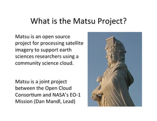
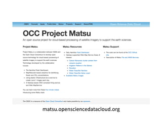
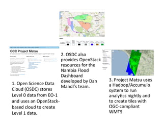
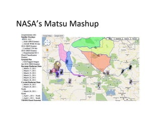
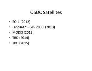
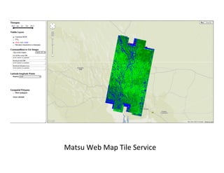
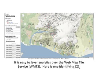
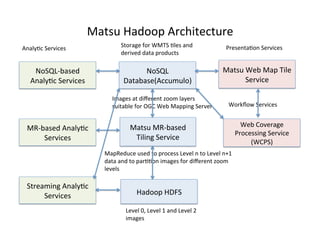
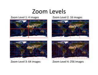
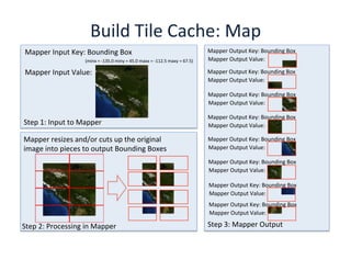
The Matsu Project is an Open Cloud Consortium project that is developing open source software for processing satellite imagery data using Hadoop, OpenStack and R.

1. The
Matsu
Project
Robert
L.
Grossman
University
of
Chicago
Open
Cloud
ConsorAum
June
18,
2013

2. The
Matsu
Project
represents
work
by
Collin
BenneL,
Robert
L.
Grossman,
MaLhew
Handy,
Vuong
Ly,
Dan
Mandl,
Ryan
Miller,
Jim
Pivarski,
Ray
Powell
and
Steve
Vejcik.

3. What
is
the
Matsu
Project?
Matsu
is
an
open
source
project
for
processing
satellite
imagery
to
support
earth
sciences
researchers
using
a
community
science
cloud.
Matsu
is
a
joint
project
between
the
Open
Cloud
ConsorAum
and
NASA’s
EO-­‐1
Mission
(Dan
Mandl,
Lead)

4. matsu.opensciencedatacloud.org

5. EO-­‐1
mission
• Approved
in
March
1996
and
launched
on
November
21,
2000
from
Vandenburg
Air
Force
Base,
California
on
a
Delta
7320
• All
technologies
were
flight-­‐validated
by
December
2001
• EO-­‐1
is
now
in
an
Extended
Mission

6. EO-­‐1’s
ALI
and
Hyperion
Instruments

7. Data
-­‐
Instruments
• Hyperion
Imaging
Spectrometer
– Designed
to
gather
data
from
a
given
region
on
the
Earth
by
viewing
the
surface
in
terms
of
242
disAnct
'bands'
of
light.
• Advanced
Land
Imager
(ALI)
– Used
to
validate
and
demonstrate
technology
for
the
Landsat
Data
ConAnuity
Mission
(LDCM)

8. All
available
L1G
images
(2010-­‐now)

9. 1.
Open
Science
Data
Cloud
(OSDC)
stores
Level
0
data
from
EO-­‐1
and
uses
an
OpenStack-­‐
based
cloud
to
create
Level
1
data.
2.
OSDC
also
provides
OpenStack
resources
for
the
Nambia
Flood
Dashboard
developed
by
Dan
Mandl’s
team.
3.
Project
Matsu
uses
a
Hadoop/Accumulo
system
to
run
analyAcs
nightly
and
to
create
Ales
with
OGC-­‐compliant
WMTS.

10. NASA’s
Matsu
Mashup

11. OSDC
Satellites
• EO-­‐1
(2012)
• Landsat7
–
GLS
2000
(2013)
• MODIS
(2013)
• TBD
(2014)
• TBD
(2015)

12. Matsu
Web
Map
Tile
Service

13. It
is
easy
to
layer
analyAcs
over
the
Web
Map
Tile
Service
(WMTS).
Here
is
one
idenAfying
CO2

14. Matsu
Hadoop
Architecture
Hadoop
HDFS
Matsu
Web
Map
Tile
Service
Matsu
MR-­‐based
Tiling
Service
NoSQL
Database(Accumulo)
Images
at
different
zoom
layers
suitable
for
OGC
Web
Mapping
Server
Level
0,
Level
1
and
Level
2
images
MapReduce
used
to
process
Level
n
to
Level
n+1
data
and
to
parAAon
images
for
different
zoom
levels
NoSQL-­‐based
AnalyAc
Services
Streaming
AnalyAc
Services
MR-­‐based
AnalyAc
Services
AnalyAc
Services
Storage
for
WMTS
Ales
and
derived
data
products
PresentaAon
Services
Web
Coverage
Processing
Service
(WCPS)
Workflow
Services

15. Zoom
Levels
Zoom
Level
1:
4
images
Zoom
Level
2:
16
images
Zoom
Level
3:
64
images
Zoom
Level
4:
256
images

16. Mapper
Input
Key:
Bounding
Box
Mapper
Input
Value:
Mapper
Output
Key:
Bounding
Box
Mapper
Output
Value:
Mapper
resizes
and/or
cuts
up
the
original
image
into
pieces
to
output
Bounding
Boxes
(minx
=
-­‐135.0
miny
=
45.0
maxx
=
-­‐112.5
maxy
=
67.5)
Step
1:
Input
to
Mapper
Step
2:
Processing
in
Mapper
Step
3:
Mapper
Output
Mapper
Output
Key:
Bounding
Box
Mapper
Output
Value:
Mapper
Output
Key:
Bounding
Box
Mapper
Output
Value:
Mapper
Output
Key:
Bounding
Box
Mapper
Output
Value:
Mapper
Output
Key:
Bounding
Box
Mapper
Output
Value:
Mapper
Output
Key:
Bounding
Box
Mapper
Output
Value:
Mapper
Output
Key:
Bounding
Box
Mapper
Output
Value:
Mapper
Output
Key:
Bounding
Box
Mapper
Output
Value:
Build
Tile
Cache:
Map

17. Reducer
Key
Input:
Bounding
Box
(minx
=
-­‐45.0
miny
=
-­‐2.8125
maxx
=
-­‐43.59375
maxy
=
-­‐2.109375)
Reducer
Value
Input:
Step
1:
Input
to
Reducer
…
Step
2:
Reducer
Output
Assemble
Images
based
on
bounding
box
• Reducer
assembles
Ales
at
each
zoom
level
• Tiles
wriLen
to
Accumulo
(a
NoSQL
database)
Build
Tile
Cache:
Reduce

18. Map
Phase
• Map
– Read
in
images
by
Bands,
Date,
and
Region
– Fix
a
zoom
level
for
sending
to
reducers
• Based
on
number
of
reducers
and
processing
power,
not
on
the
zoom
you
want
for
display
– Emit
as
<key>,
<value>
• Key
=
<Bounding
Box
at
Fixed
Zoom
Level>
• Value
=
<Bounding
Bounding
Box
at
Smallest
Zoom
Level,
Bands,
ProjecAon,
Timestamp,
Image
Bytes>

19. Reduce
Phase
• All
bytes
for
bands
and
satellite
strips
in
this
bounding
box
are
mapped
to
the
same
reducer
• The
key
can
be
idenAfied
by
the
Lat/Long
of
the
upper
right
corner
of
the
box

20. Level
1
Images
-­‐
Details
• Satellite
track
images
(L1R)
are
rotated
and
geolocated
(L1G)
by
NASA
• We
overlay
L1G
images
into
Level-­‐2
dyadic
Ales
in
Map-­‐Reduce
locaAon
in
Google
Maps
L1R
L1G
Level-­‐2
Ales
made
in
Map-­‐Reduce,
prepared
for
WMS
T06-­‐00097-­‐00092
T10-­‐01561-­‐01486

21. Some
example
images
Gobi
Desert
• same
as
previous
page
• contains
some
strange
structures
that
are
too
small
to
spaAally
resolve
with
Hyperion,
but
they
might
have
interesAng
spectral
features

22. Some
example
images
Karijini,
Australia
• lots
of
colorful
minerals
• should
have
a
very
rich
spectrum

23. Some
example
images
Lake
Frome,
Australia
• salt
bed
is
a
standard
calibraAon
target
Atacama
Desert,
Chile
• salt
bed
in
the
driest
part
of
the
world

24. • CO2
has
three
absorbAon
lines
within
Hyperion’s
spectral
range
• Sideband
subtracAon
technique
extracts
a
pure
sample
of
data
in
a
peak
by
fisng
nearby
datapoints
to
a
curve
and
subtracAng
peak
values
from
the
curve
• In
this
case,
we
invert
the
subtracAon
because
it’s
an
anA-­‐
peak
External
Reference
Algebraic
combinaAon
of
spectral
bands
to
make
a
more
sensiAve
image

25. • CO2
has
three
absorbAon
lines
within
Hyperion’s
spectral
range
• Sideband
subtracAon
technique
extracts
a
pure
sample
of
data
in
a
peak
by
fisng
nearby
datapoints
to
a
curve
and
subtracAng
peak
values
from
the
curve
• In
this
case,
we
invert
the
subtracAon
because
it’s
an
anA-­‐
peak
Algebraic
combinaAon
of
spectral
bands
to
make
a
more
sensiAve
image
two
bands
in
the
CO2
line

26. Algebraic
combinaAon
of
spectral
bands
to
make
a
more
sensiAve
image
• Icelandic
volcano
in
April
2010
(Eyjatallajökull)
• Visible
frame
is
full
of
ash
clouds
• CO2
distribuAon
is
non-­‐uniform
• Some
CO2
acAvity
follows
visible
cloud
formaAons,
some
doesn’t

27. Algebraic
combinaAon
of
spectral
bands
to
make
a
more
sensiAve
image
• Some
CO2
acAvity
follows
visible
cloud
formaAons,
some
doesn’t
Python
code
used
to
produce
this
image
(vectors
in
bold):
sum1
=
4.
sumx
=
183.
+
184.
+
188.
+
189.
sumxx
=
183.**2
+
184.**2
+
188.**2
+
189.**2
sumy
=
B183
+
B184
+
B188
+
B189
sumxy
=
183.*B183
+
184.*B184
+
188.*B188
+
189.*B189
delta
=
sum1*sumxx
-­‐
sumx**2
constant
=
(sumxx*sumy
-­‐
sumx*sumxy)
/
delta
linear
=
(sum1*sumxy
-­‐
sumx*sumy)
/
delta
subtracted
=
(B185
-­‐
(constant
+
185.*linear))/2.
+
(B186
-­‐
(constant
+
186.*linear))/2.
• Icelandic
volcano
in
April
2010
(Eyjatallajökull)
• Visible
frame
is
full
of
ash
clouds
• CO2
distribuAon
is
non-­‐uniform

28. Algebraic
combinaAon
of
spectral
bands
to
make
a
more
sensiAve
image
• Some
CO2
acAvity
follows
visible
cloud
formaAons,
some
doesn’t
hLp://lvoc-­‐matsu.opensciencedatacloud.org/SimpleWMS/?
lat=63.7&lng=-­‐19.45&z=11&rgb=true&co2=true&flood=false&points=clust
ers
• Icelandic
volcano
in
April
2010
(Eyjatallajökull)
• Visible
frame
is
full
of
ash
clouds
• CO2
distribuAon
is
non-­‐uniform

29. QuesAons

30. For
More
InformaAon
• Project
Matsu
is
managed
and
operated
by
the
Open
Cloud
ConsorAum
(www.opencloudconsorAum.org).
• Project
Matsu
is
supported
in
part
by
grants
from
Gordon
and
BeLy
Moore
FoundaAon
and
the
NaAonal
Science
FoundaAon
(Grants
OISE
-­‐
1129076
and
CISE
1127316).
• For
more
informaAon
about
Project
Matsu,
please
see
the
Project
Matsu
website:
matsu.opensciencedatacloud.org
• The
Project
Director
is
Robert
Grossman,
who
can
be
reached
at

31. Here
is
some
detail
of
how
we
process
EO-­‐1
satellite
imagery
data
using
Hadoop
in
Project
Matsu…

32. Step
1
–
Storage
&
Archiving
From
Space
to
Goddard
to
the
OSDC
1. Transmit
data
from
NASA’s
EO-­‐1
Satellite
to
NASA
ground
staAons
and
then
to
NASA
Goddard
2. At
Goddard,
align
data,
perform
radiometric
correcAons
and
generate
Level
0
images
(16-­‐bit
radiance
values)
3. Transmit
Level
0
data
from
NASA
Goddard
to
the
OCC’s
Open
Science
Data
Cloud
(OSDC)
4. Store
images
in
a
distributed,
fault
tolerate,
file
system

33. Step
2
–
CreaAng
Level
1
Images
Building
Level
1
Images
on
the
OSDC
1. Each
day,
the
new
Level
0
images
stored
on
the
OSDC
are
processed
2. Within
the
OSDC,
NASA
launches
Virtual
Machines
(VMs)
specifically
built
to
render
Level
1
images
from
Level
0
data.
– Each
Level
1
band
is
saved
as
a
disAnct
image
3. Level
1
bands
are
wriLen
to
storage
facility
in
the
OSCD
for
long-­‐term
public
access

34. Step
3
–
Tiling
Matsu
Processing
1. Build
Web
Mapping
Tile
Service
Tiles
from
Level
1
images
using
MapReduce
2. Store
Ales
in
Accumulo
• Index
them
so
that
they
are
accessible
via
Web
Mapping
Service
3. Run
AnalyAcs
on
Level
1
images
• Move
results
of
the
analyAcs
to
Accumulo

35. Tiling
-­‐
Detail
• Use
MapReduce
to
build
Web
Tiles
1. Each
day,
the
Level
1
images
created
by
NASA
and
stored
on
the
OSDC
are
processed
2. The
Date
and
Bands
(to
create
a
visible
image)
are
specified
3. Run
MapReduce
Job
1. Map
–
FILL-­‐IN
2. ParAAon
–
FILL-­‐IN
3. Reduce
–
FILL-­‐IN

36. Tile
Details,
cont’d
• Images
are
handles
as
byte
streams
• Divide
(chunk)
the
Level
1
images
into
manageable
sizes.
• Dyadic
decomposiAon
– Divide
each
image
into
4
equal
size
pieces
– For
each
addiAonal
zoom,
subdivide
each
piece
into
4
equal
size
pieces
• Tag
each
chunked
images
with
the
bounding
box,
date,
Ame,
dyadic
level
and
bands.
• Convert
the
bytes
into
PNG
files

37. Processing
the
Data
• Reduce
– Once
all
images
are
received
for
a
Bounding
Box,
sort
by
the
most
granular
zoom
level
– Process
that
Zoom
Level
– Once
a
zoom
level
in
is
completed,
combine
images
and
scale
the
build
the
next
zoom
level
Z1
Z1
Z1
Z1
Z2
Z2
1.
Assemble
2.
Scale

38. Accumulo
Storage
• Images
are
stored
by
Bounding
Box
– -­‐180.0_-­‐90.0_180.0_90.0
• Column
family
– The
Ale
style,
zoom,
and
projecAon
• Column
qualifier
– Dimensions
(width
and
height,
512
x
256)
• Value
– the
corresponding
PNG
image
in
raw
bytes

39. Serve
to
WMTS
• The
WMTS
query:
– Bounding
Box
– Date
– Layer
name
as
a
string
• HaiA
– Style
name
as
a
string
• The
bands
used
to
build
the
Level
1
image
or
an
alias:
“B058:B023:B015”
or
“agricultural”
• Not
supported
– Map
Project
could
be
used,
but
for
now,
we
only
support
a
single
projecAon

40. Images:
stages
of
processing
• Satellite
track
images
(L1R)
are
rotated
and
geolocated
(L1G)
by
NASA
• We
overlay
L1G
images
into
Level-­‐2
dyadic
Ales
using
Map-­‐Reduce
image
locaAons
(viewed
in
Google
Maps)
L1R
L1G
Level-­‐2
Ales
made
in
Map-­‐Reduce,
prepared
for
WMS
T06-­‐00097-­‐00092
T10-­‐01561-­‐01486