CMSIハンズオン資料

1. ALPS チュートリアル: Introduction to Matplotlib
ALPS チュートリアル: Introduction to
Matplotlib
CMSI ハンズオン
ALPS Collaboration
http://alps.comp-phys.org/
2014-10-16
1 / 9

2. ALPS チュートリアル: Introduction to Matplotlib
Outline
1 環境設定
2 プロットしてみる
3 Figure とAxes
2 / 9

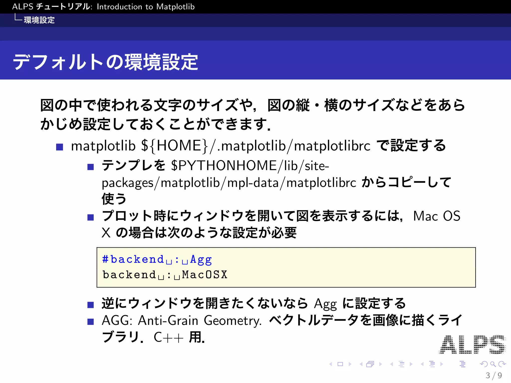
3. ALPS チュートリアル: Introduction to Matplotlib
環境設定
デフォルトの環境設定
図の中で使われる文字のサイズや，図の縦・横のサイズなどをあら
かじめ設定しておくことができます．
matplotlib $fHOMEg/.matplotlib/matplotlibrc で設定する
テンプレを$PYTHONHOME/lib/site-
packages/matplotlib/mpl-data/matplotlibrc からコピーして
使う
プロット時にウィンドウを開いて図を表示するには，Mac OS
X の場合は次のような設定が必要
#backend : Agg
backend : MacOSX
逆にウィンドウを開きたくないならAgg に設定する
AGG: Anti-Grain Geometry. ベクトルデータを画像に描くライ
ブラリ．C++ 用．
3 / 9

4. ALPS チュートリアル: Introduction to Matplotlib
環境設定
動的に環境設定を行う
backend の設定はimport matplotlib の直後にすること
>>> import matplotlib as mpl
>>> mpl.use('Agg')
グラフのサイズやフォントのサイズの設定
>>> import pylab
>>> params = {
... 'legend.fontsize': 10
... 'xtick.labelsize': 8
... 'ytick.labelsize': 8
... 'figure.figsize': [width, height]}
>>> pyalps.rcParams.update(params)
4 / 9

5. ALPS チュートリアル: Introduction to Matplotlib
プロットしてみる
簡単な図をプロットしてみる
y = x2 のプロット
>>> x = range(-10,10)
>>> y = [i*i for i in x]
# シンボルの色を赤(r)，
# 形を丸(o)に設定
>>> pl.plot(x, y, 'ro')
...[<matplotlib.lines.Line2D at 0
x114c82710>]
# 拡張子で保存の
# ファイル形式が決まります!
>>> pl.savefig('x2.pdf')
>>> pl.show()
10 5 0 5 10
100
80
60
40
20
0
5 / 9

6. ALPS チュートリアル: Introduction to Matplotlib
プロットしてみる
少し複雑な図をプロットしてみる
>>> import math as m # cos を使うため
>>> x = range(-10,10)
>>> y1 = [i*i for i in x]
>>> y2 = [i*i*i for i in x]
>>> y3 = [m.cos(2 * m.pi * i/20) for i in x]
# 図を上下2 段に並べてプロットします
>>> pl.subplot(211) # 上側の図を書き始めます
>>> pl.plot(x, y1, 'ro') # 1 つのグラフに
>>> pl.plot(x, y2, 'b^') # 2 つのデータセットをプロット
>>> pl.title('$x^2$ and $x^3$') # 図のタイトル．TeX もOk!
>>> pl.legend(('$y1$', '$y2$'), numpoints=1) # 凡例
6 / 9

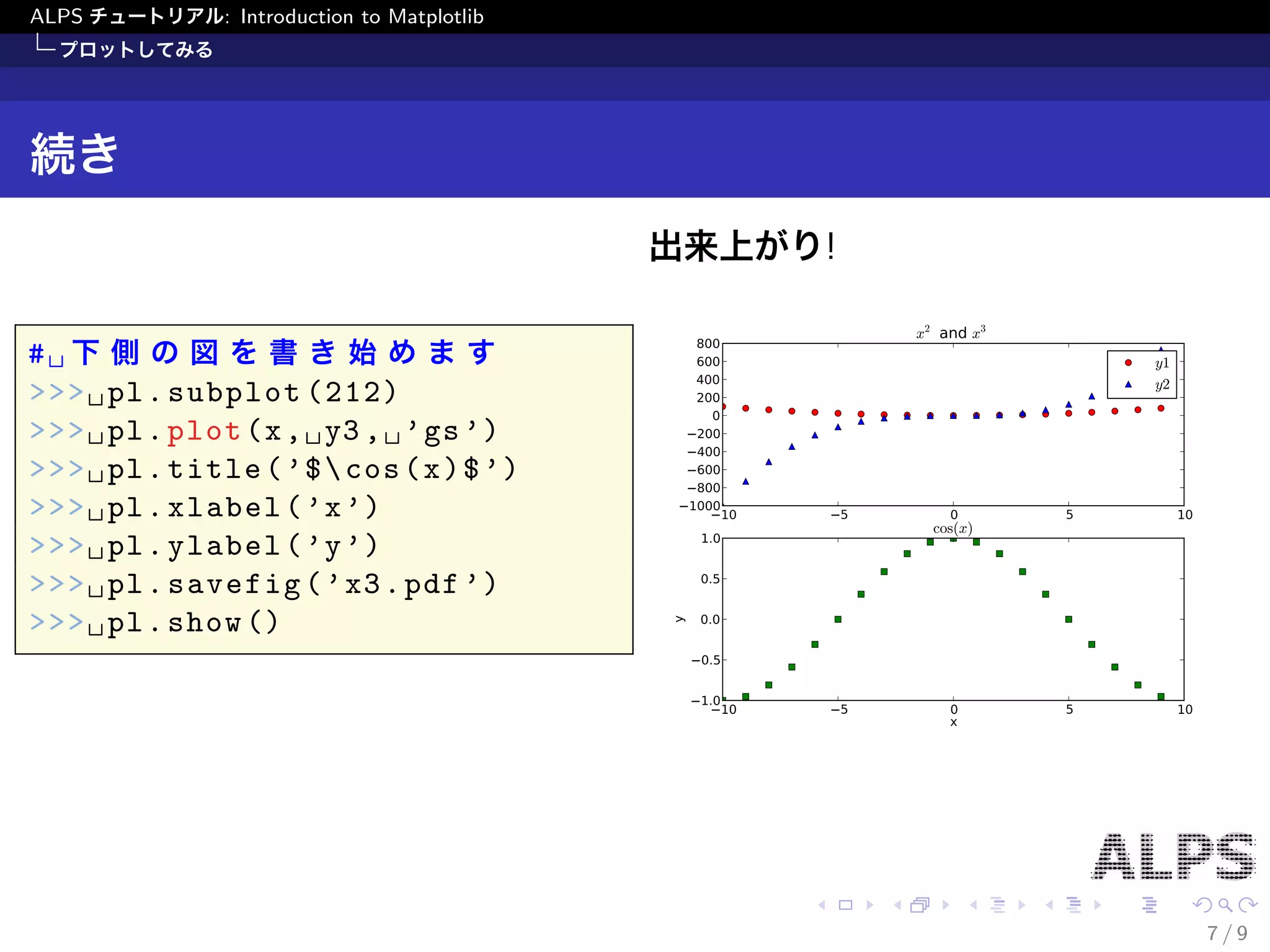
7. ALPS チュートリアル: Introduction to Matplotlib
プロットしてみる
続き
# 下側の図を書き始めます
>>> pl.subplot(212)
>>> pl.plot(x, y3, 'gs')
>>> pl.title('$cos(x)$')
>>> pl.xlabel('x')
>>> pl.ylabel('y')
>>> pl.savefig('x3.pdf')
>>> pl.show()
出来上がり!
10 5 0 5 10
800
600
400
200
0
200
400
600
800
1000
x2 and x3
y1
y2
10 5 0 5 10
x
1.0
0.5
0.0
0.5
1.0
y
cos(x)
7 / 9

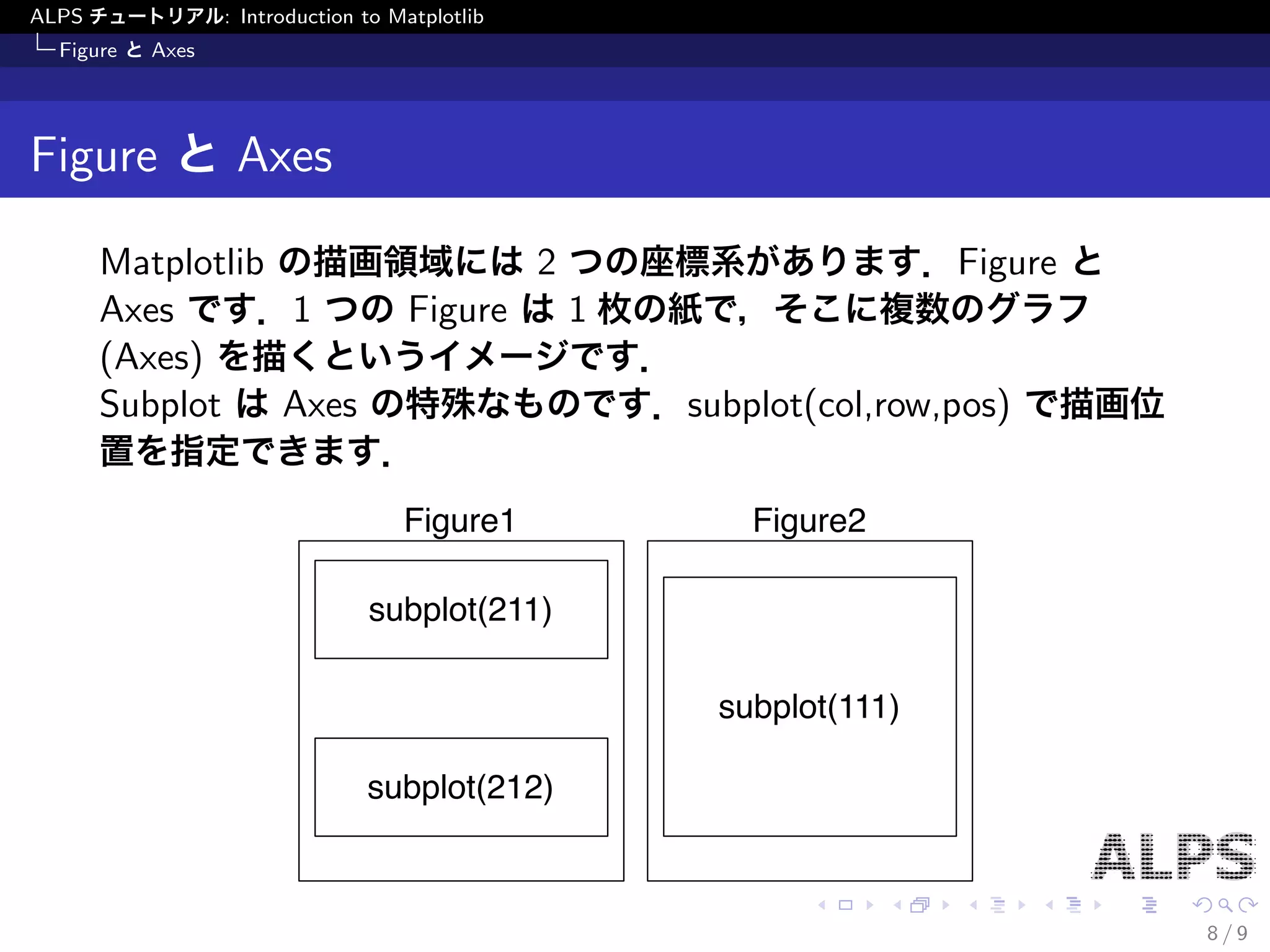
8. ALPS チュートリアル: Introduction to Matplotlib
Figure とAxes
Figure とAxes
Matplotlib の描画領域には2 つの座標系があります．Figure と
Axes です．1 つのFigure は1 枚の紙で，そこに複数のグラフ
(Axes) を描くというイメージです．
Subplot はAxes の特殊なものです．subplot(col,row,pos) で描画位
置を指定できます．
Figure1 Figure2
subplot(211)
subplot(212)
subplot(111)
8 / 9

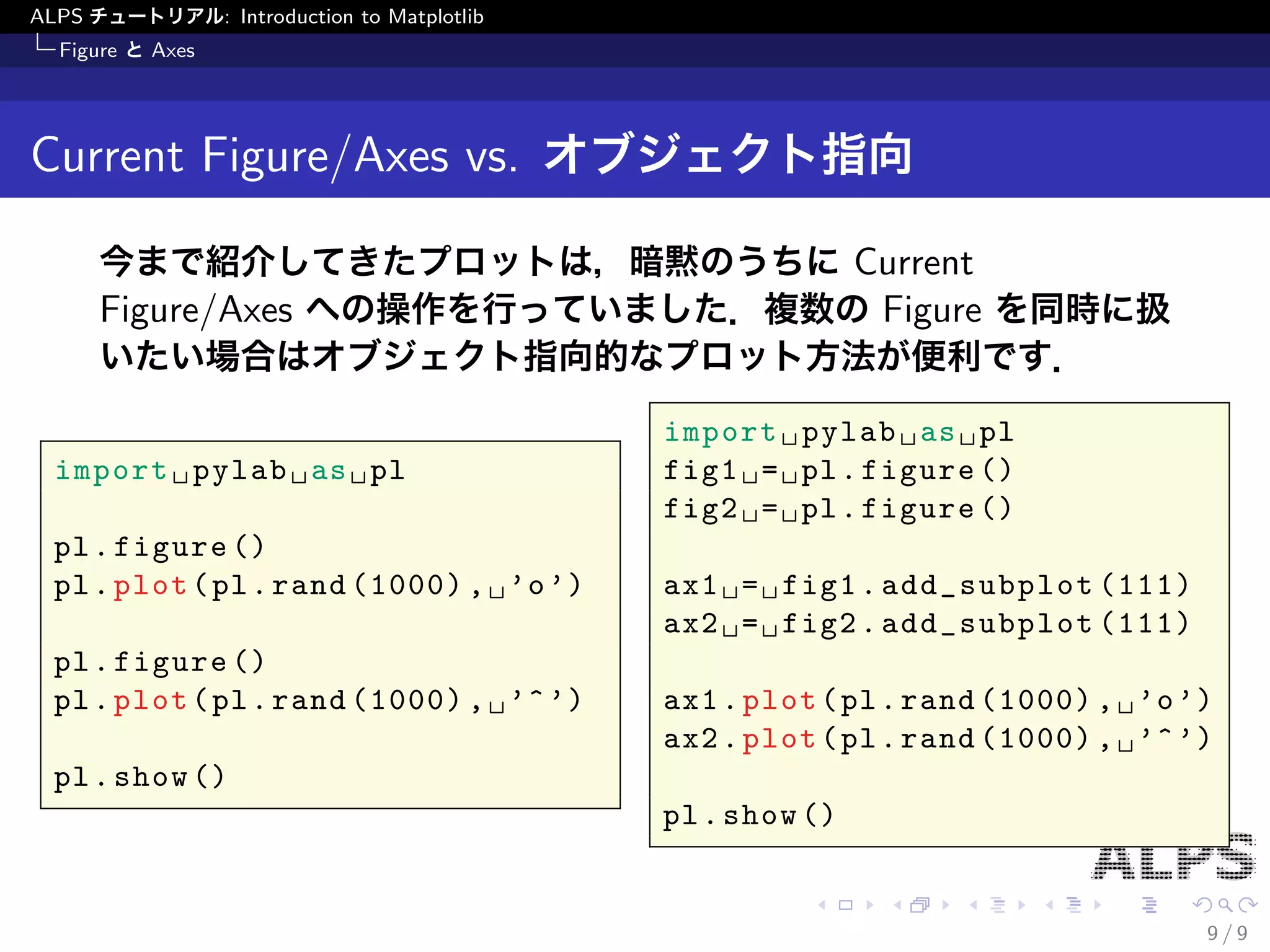
9. ALPS チュートリアル: Introduction to Matplotlib
Figure とAxes
Current Figure/Axes vs. オブジェクト指向
今まで紹介してきたプロットは，暗黙のうちにCurrent
Figure/Axes への操作を行っていました．複数のFigure を同時に扱
いたい場合はオブジェクト指向的なプロット方法が便利です．
import pylab as pl
pl.figure()
pl.plot(pl.rand(1000), 'o')
pl.figure()
pl.plot(pl.rand(1000), '^')
pl.show()
import pylab as pl
fig1 = pl.figure()
fig2 = pl.figure()
ax1 = fig1.add_subplot(111)
ax2 = fig2.add_subplot(111)
ax1.plot(pl.rand(1000), 'o')
ax2.plot(pl.rand(1000), '^')
pl.show()
9 / 9