MATLAB’de GRAFİK İŞLEMLERİ
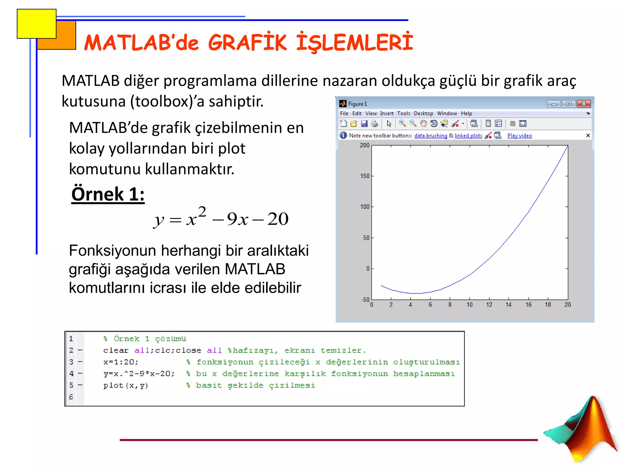
MATLABdiğer programlama dillerine nazaran oldukça güçlü bir grafik araç
kutusuna (toolbox)’a sahiptir.
MATLAB’de grafik çizebilmenin en
kolay yollarından biri plot
komutunu kullanmaktır.
Örnek 1:
2092
xxy
Fonksiyonun herhangi bir aralıktaki
grafiği aşağıda verilen MATLAB
komutlarını icrası ile elde edilebilir
3.
GRAFİK DÜZENLEYEN KOMUTLAR
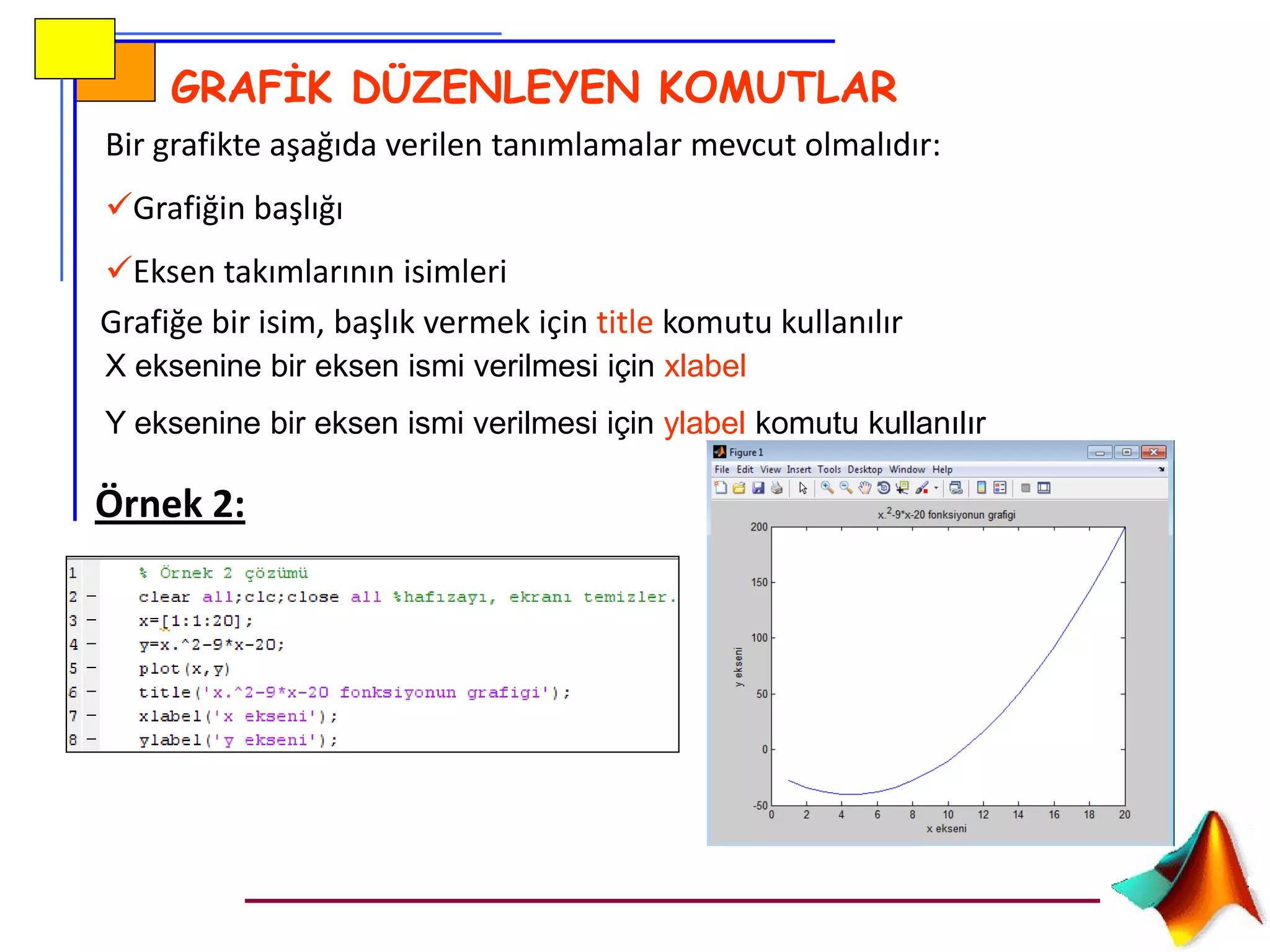
Birgrafikte aşağıda verilen tanımlamalar mevcut olmalıdır:
Grafiğin başlığı
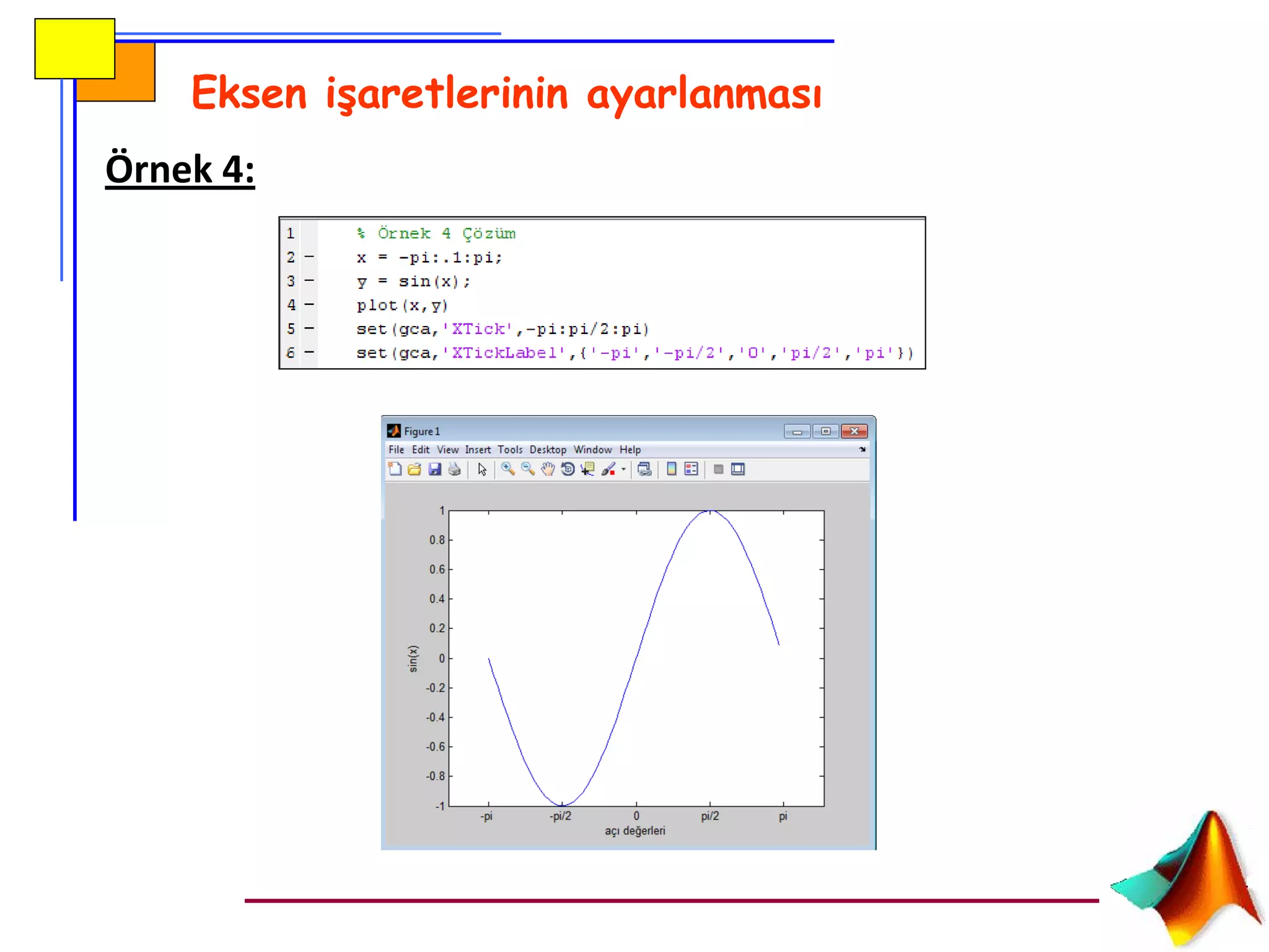
Eksen takımlarının isimleri
Grafiğe bir isim, başlık vermek için title komutu kullanılır
X eksenine bir eksen ismi verilmesi için xlabel
Y eksenine bir eksen ismi verilmesi için ylabel komutu kullanılır
Örnek 2:
4.
ÇOKLU GRAFİKLER
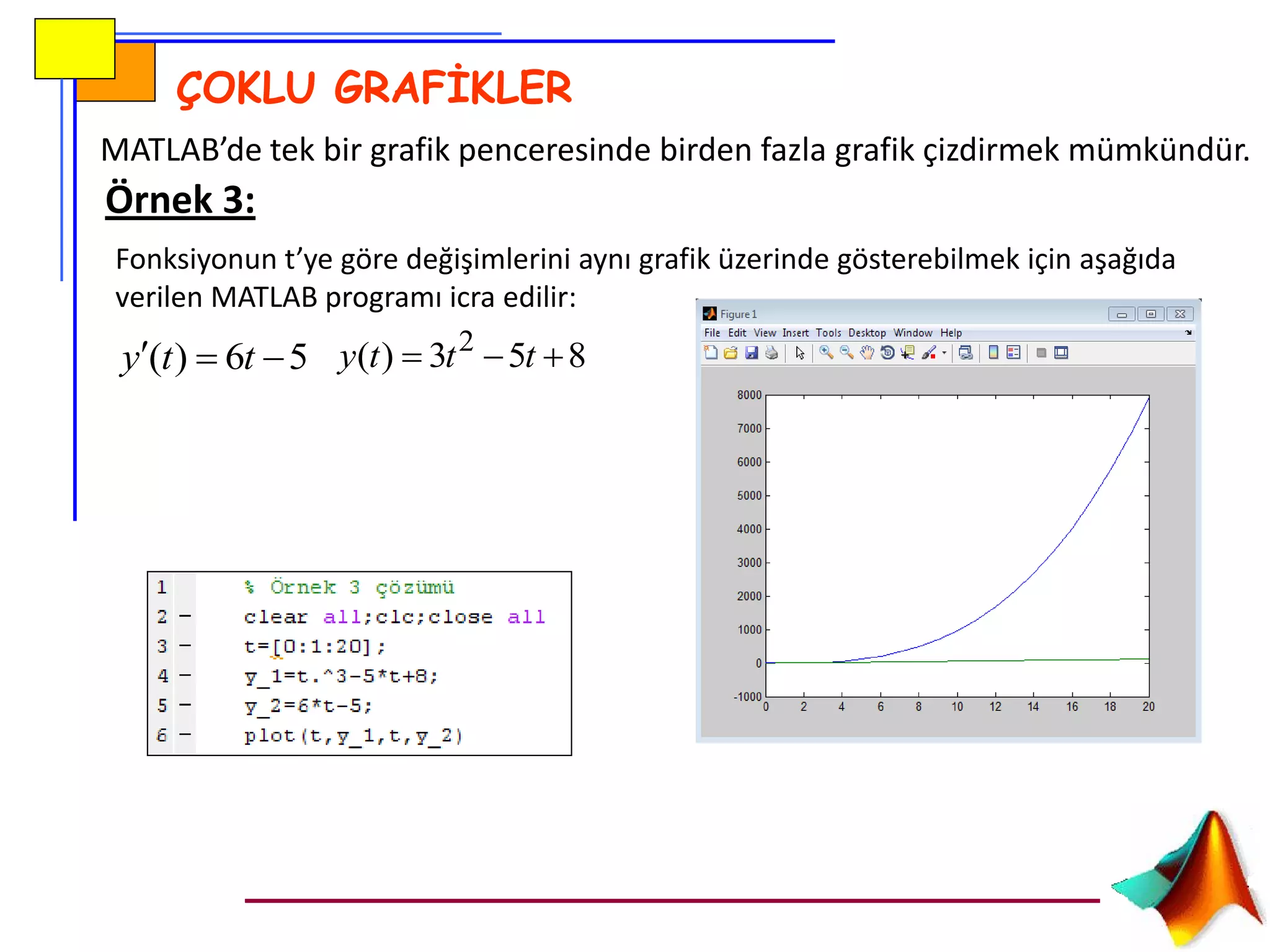
MATLAB’de tekbir grafik penceresinde birden fazla grafik çizdirmek mümkündür.
853)( 2
ttty56)( tty
Fonksiyonun t’ye göre değişimlerini aynı grafik üzerinde gösterebilmek için aşağıda
verilen MATLAB programı icra edilir:
Örnek 3:
GRAFİKLERDE ÇEŞİTLİ DÜZENLEMELER
Eldeedilen grafiklerde aşağıda belirtilen düzenlemeler yapılabilir:
çizgi rengi ve tipini değiştirmek
x değişkeni ile fonksiyon değerinin kesişitiği noktaların işaretlemek
Grafiklere açıklama eklemek
Plot(x,y,’r-’) şeklindeki bir komut ile x ve y vektörlerinin grafik çizgi
renginin kırmızı ve düz bir çizgi olması sağlanır.
7.
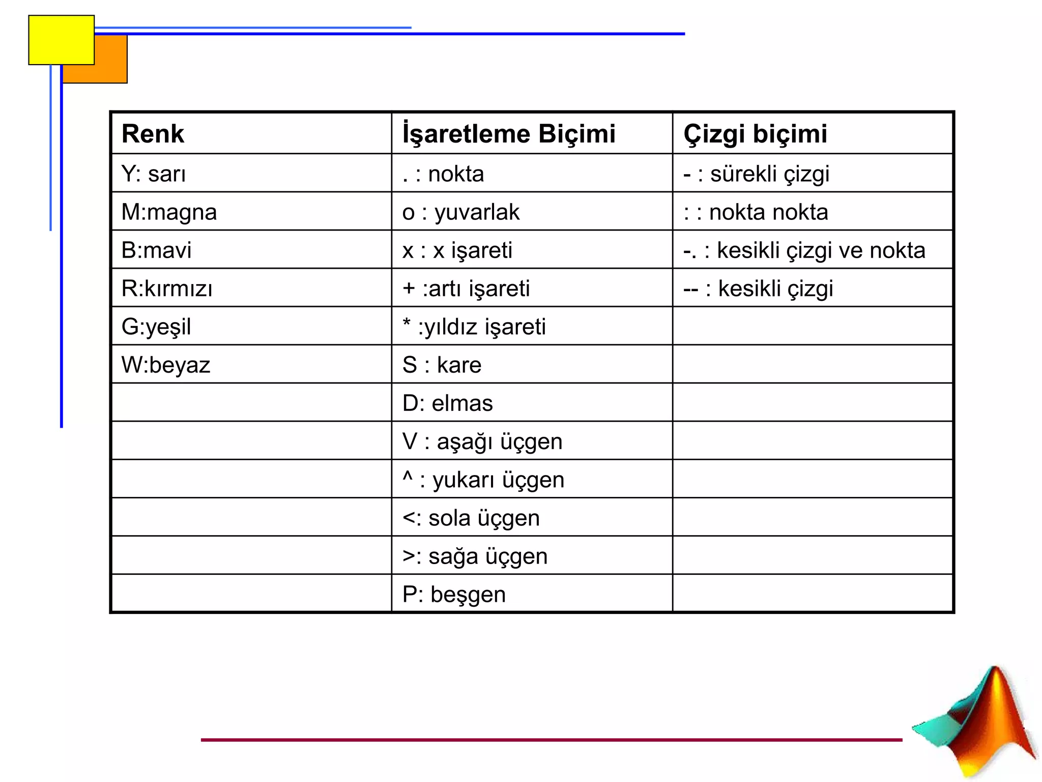
Renk İşaretleme BiçimiÇizgi biçimi
Y: sarı . : nokta - : sürekli çizgi
M:magna o : yuvarlak : : nokta nokta
B:mavi x : x işareti -. : kesikli çizgi ve nokta
R:kırmızı + :artı işareti -- : kesikli çizgi
G:yeşil * :yıldız işareti
W:beyaz S : kare
D: elmas
V : aşağı üçgen
^ : yukarı üçgen
<: sola üçgen
>: sağa üçgen
P: beşgen
8.
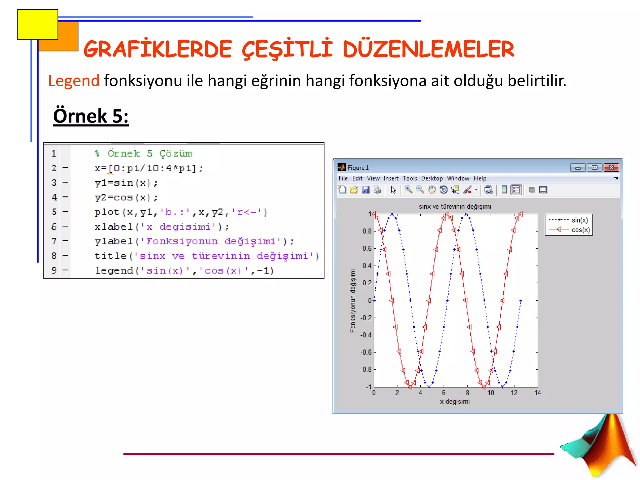
Legend fonksiyonu ilehangi eğrinin hangi fonksiyona ait olduğu belirtilir.
GRAFİKLERDE ÇEŞİTLİ DÜZENLEMELER
Örnek 5:
9.
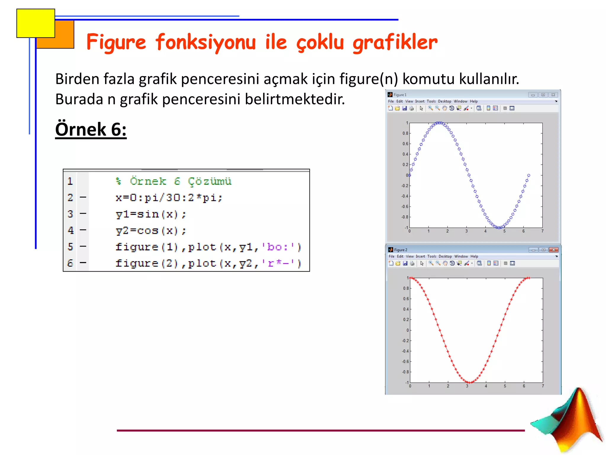
Figure fonksiyonu ileçoklu grafikler
Birden fazla grafik penceresini açmak için figure(n) komutu kullanılır.
Burada n grafik penceresini belirtmektedir.
Örnek 6:
10.
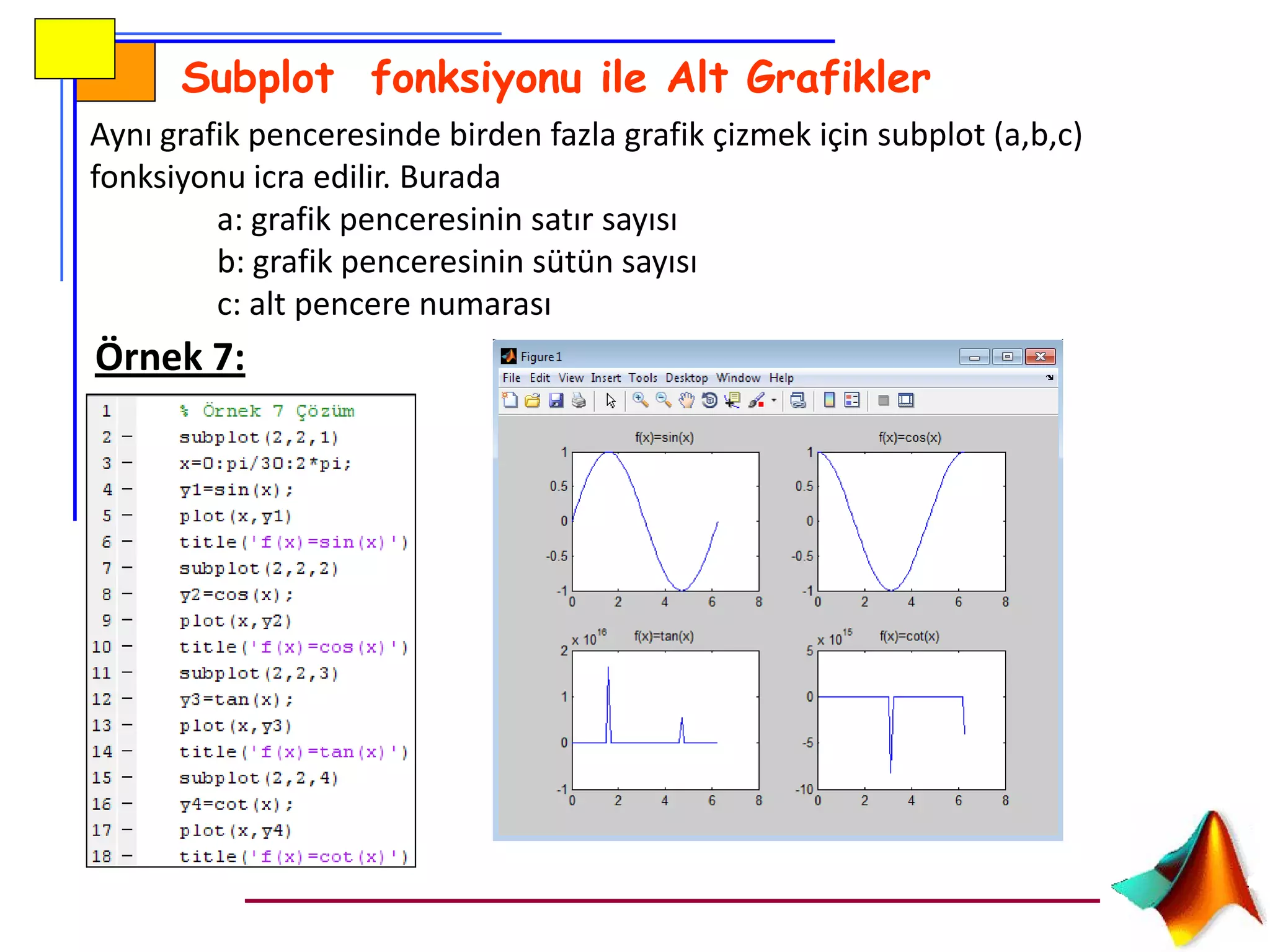
Subplot fonksiyonu ileAlt Grafikler
Aynı grafik penceresinde birden fazla grafik çizmek için subplot (a,b,c)
fonksiyonu icra edilir. Burada
a: grafik penceresinin satır sayısı
b: grafik penceresinin sütün sayısı
c: alt pencere numarası
Örnek 7:
11.
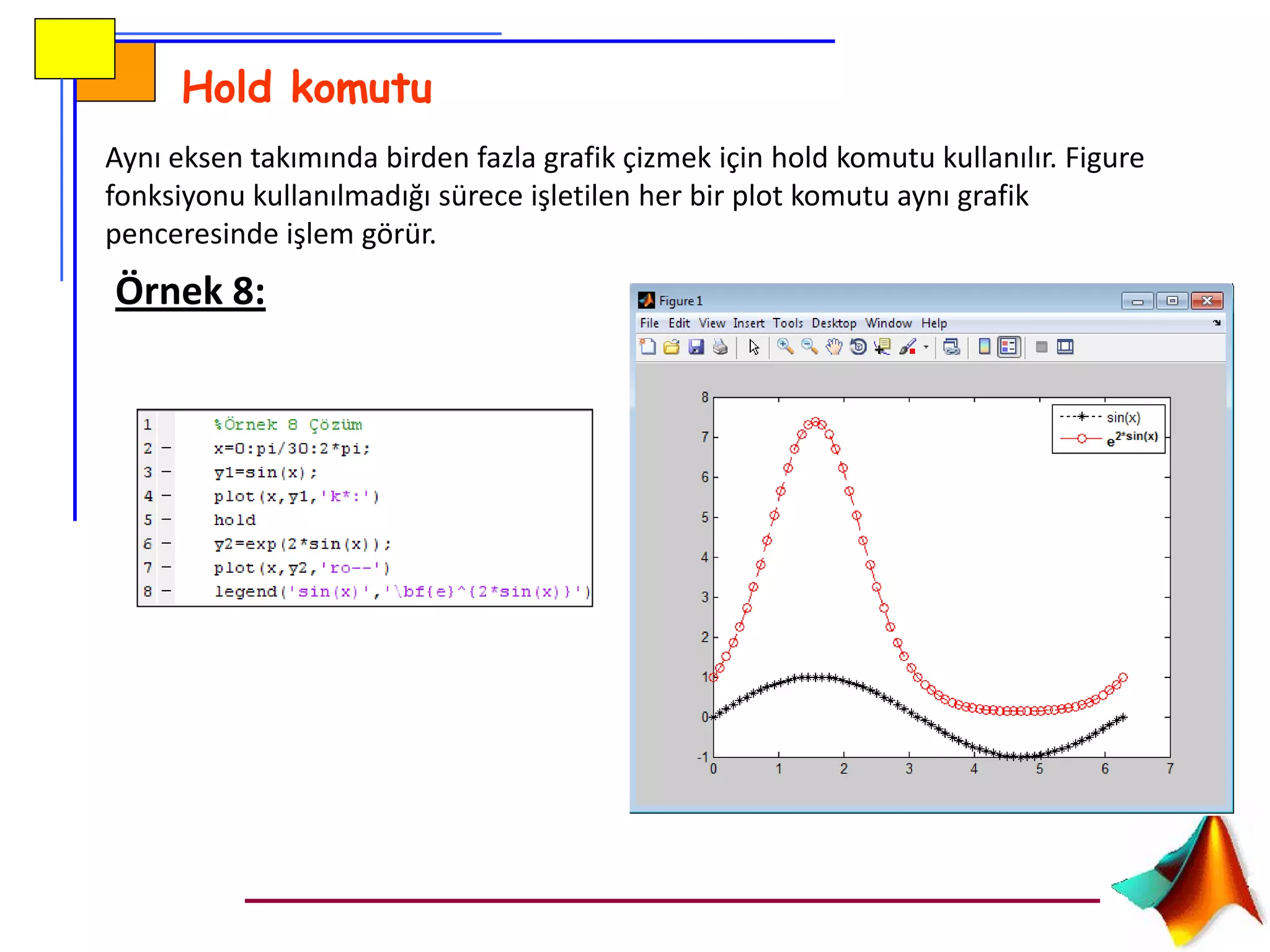
Hold komutu
Aynı eksentakımında birden fazla grafik çizmek için hold komutu kullanılır. Figure
fonksiyonu kullanılmadığı sürece işletilen her bir plot komutu aynı grafik
penceresinde işlem görür.
Örnek 8:
12.
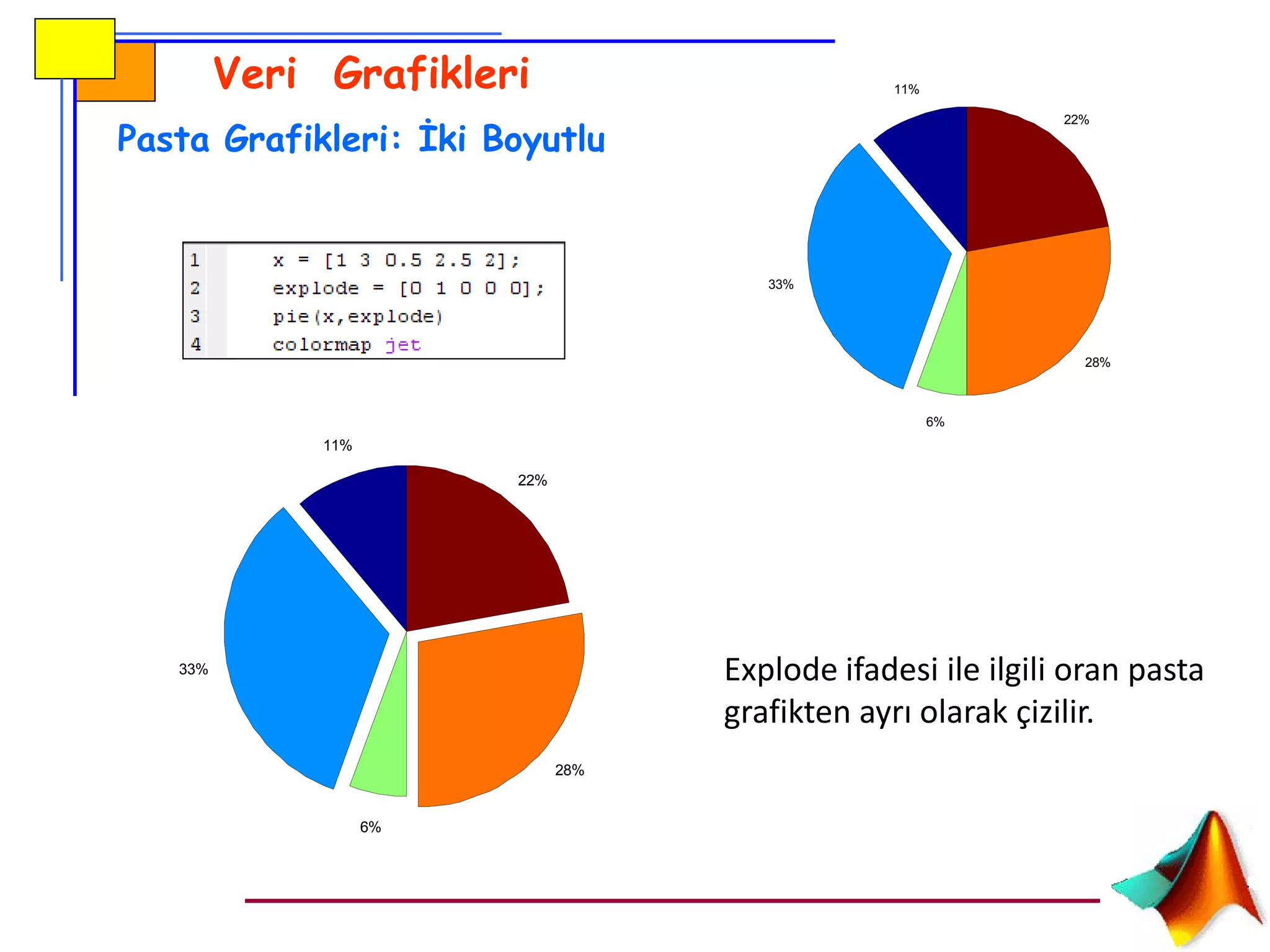
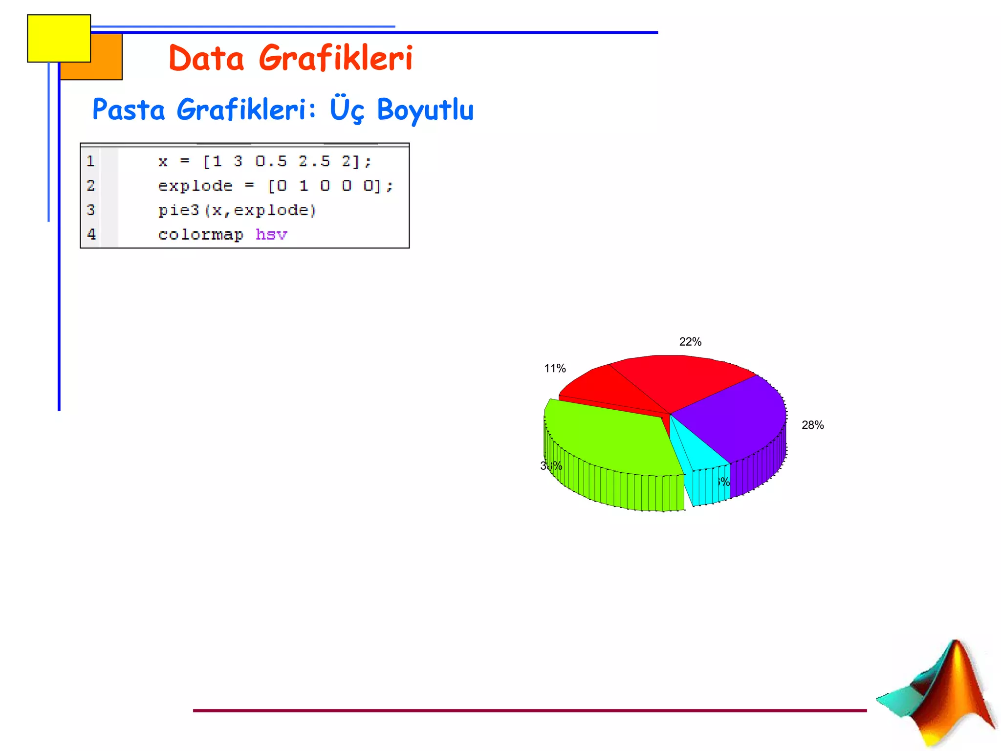
Veri Grafikleri
Pasta Grafikleri:İki Boyutlu
11%
33%
6%
28%
22%
Explode ifadesi ile ilgili oran pasta
grafikten ayrı olarak çizilir.
11%
33%
6%
28%
22%
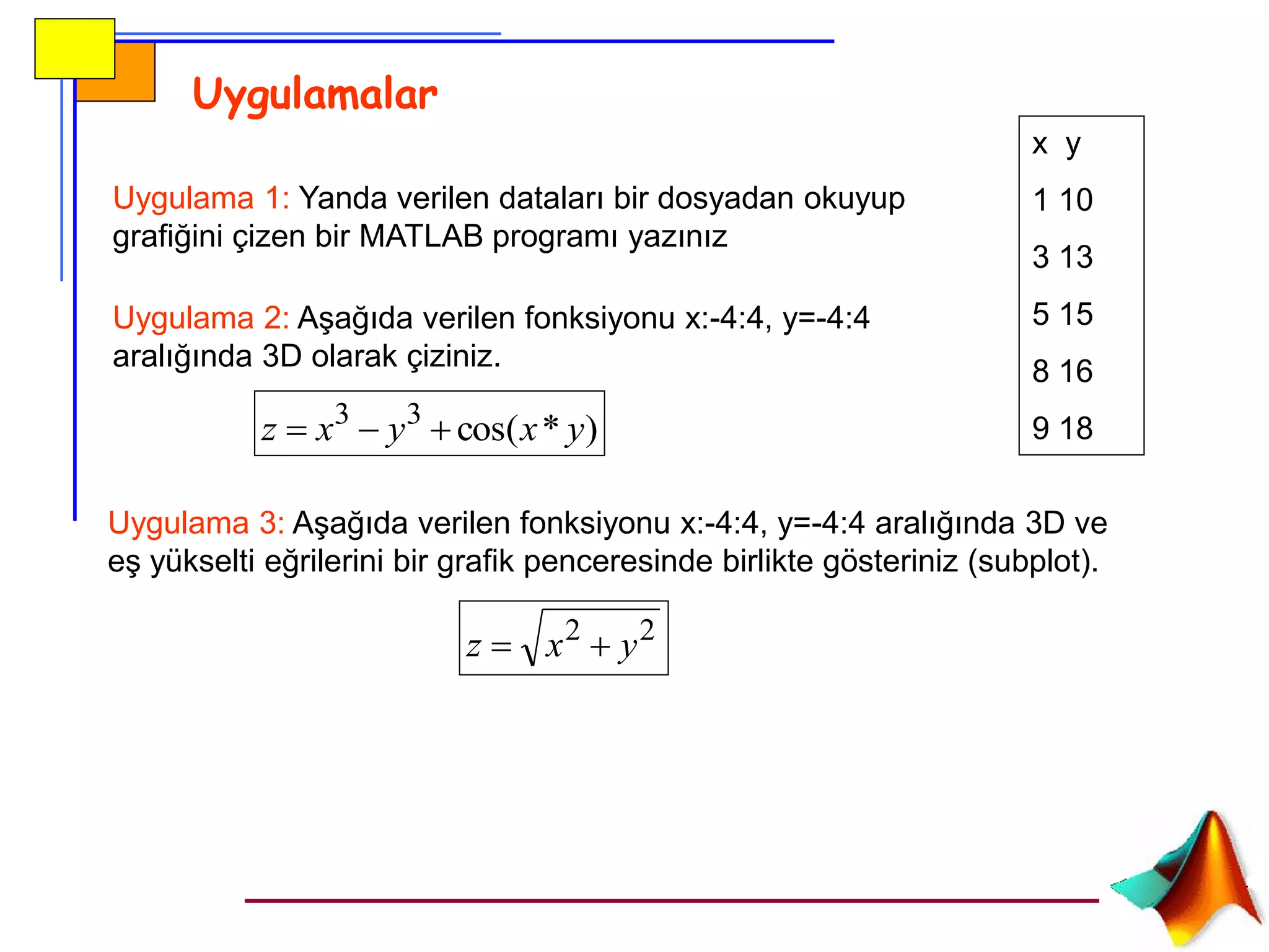
Uygulamalar
Uygulama 1: Yandaverilen dataları bir dosyadan okuyup
grafiğini çizen bir MATLAB programı yazınız
x y
1 10
3 13
5 15
8 16
9 18
Uygulama 2: Aşağıda verilen fonksiyonu x:-4:4, y=-4:4
aralığında 3D olarak çiziniz.
)*cos(33
yxyxz
Uygulama 3: Aşağıda verilen fonksiyonu x:-4:4, y=-4:4 aralığında 3D ve
eş yükselti eğrilerini bir grafik penceresinde birlikte gösteriniz (subplot).
22
yxz

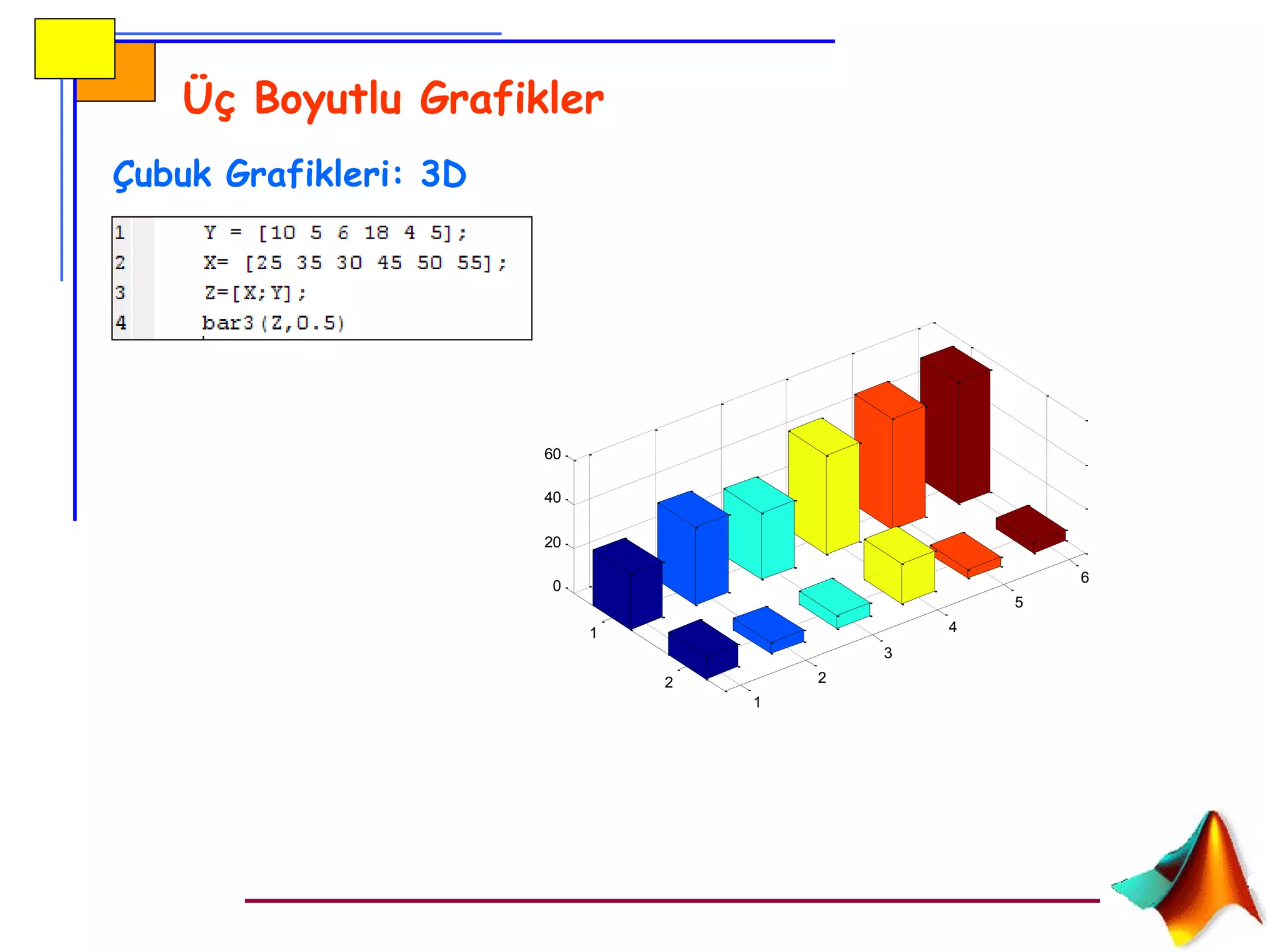
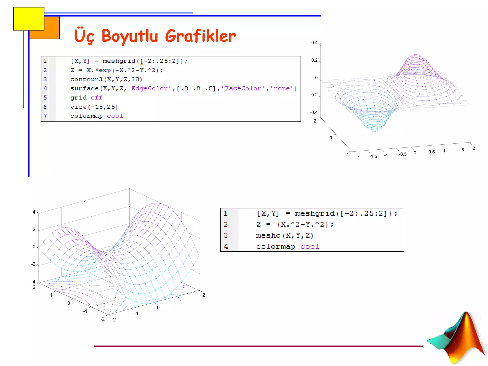
![Üç Boyutlu Grafikler
Eş yükselti eğrileri
[X,Y] = meshgrid(-2:.2:2,-2:.2:3);
Z = X.*exp(-X.^2-Y.^2);
[C,h] = contour(X,Y,Z);
clabel(C,h)
colormap cool
-2 -1.5 -1 -0.5 0 0.5 1 1.5 2
-2
-1.5
-1
-0.5
0
0.5
1
1.5
2
2.5
3
-0.4
-0.3
-0.3
-0.2
-0.2
-0.2
-0.1
-0.1
-0.1
-0.1
000
0.1
0.1
0.1
0.1
0.2
0.2
0.2
0.3
0.3
0.4](https://image.slidesharecdn.com/matlabgrafik-140617150235-phpapp01/75/Matlab-grafik-15-2048.jpg)