Machine_Learning_Co__

Covers Entire Syllabus
Question - Answer Format
Exact Answers and Solutions
Written by Popular Authors of Text Books of Technical Publications
Machine Learning
· (End Sem)
· (In Sem)
SOLVED SPPU QUESTION PAPERS
Dec 2023
july -2023

SYLLABUS
MACHINE LEARNING (410250)
Unit I : Introduction to Machine Learning
Classic and adaptive machines, Machine learning matters, Beyond machine
learning-deep learning and bio inspired adaptive systems, Machine learning and Big
data. Important Elements of Machine Learning - Data formats, Learnability, Statistical
learning approaches, Elements of information theory. (Chapter - 1)
Unit II : Feature Selection
Scikit- learn Dataset, Creating training and test sets, managing categorical data,
Managing missing features, Data scaling and normalization, Feature selection and
Filtering, Principle Component Analysis(PCA)-non negative matrix factorization, Sparse
PCA, Kernel PCA. Atom Extraction and Dictionary Learning. (Chapter - 2)
Unit III : Regression
Linear regression - Linear models, A bi-dimensional example, Linear Regression and
higher dimensionality, Ridge, Lasso and ElasticNet, Robust regression with random
sample consensus, Polynomial regression, Isotonic regression,
Logistic regression - Linear classification, Logistic regression, Implementation and
Optimizations, Stochastic gradient descendent algorithms, Finding the optimal
hyper-parameters through grid search, Classification metric, ROC Curve. (Chapter - 3)
Unit IV : Naïve Bayes and Support Vector Machine
Bayes' Theorem, Naïve Bayes. Classifiers, Naïve Bayes in Scikit- learn- Bernoulli Naïve
Bayes, Multinomial Naïve Bayes, and Gaussian Naïve Bayes. Support Vector
Machine(SVM) - Linear Support Vector Machines, Scikit - learn implementation -
Linear Classification, Kernel based classification, Non - linear Examples. Controlled
Support Vector Machines, Support Vector Regression. (Chapter - 4)
Unit V : Decision Trees and Ensemble Learning
Decision Trees - Impurity measures, Feature Importance. Decision Tree Classification
with Scikit-learn, Ensemble Learning-Random Forest, AdaBoost, Gradient Tree
Boosting, Voting Classifier.
Clustering Fundamentals - Basics, K-means : Finding optimal number of clusters,
DBSCAN, Spectral Clustering. Evaluation methods based on Ground Truth-
Homogeneity, Completeness, Adjusted Rand Index.
Introduction to Meta Classifier : Concepts of Weak and eager learner, Ensemble
methods, Bagging, Boosting, Random Forests. (Chapter - 5)
Unit VI : Clustering Techniques
Hierarchical Clustering, Expectation maximization clustering, Agglomerative Clustering-
Dendrograms, Agglomerative clustering in Scikit- learn, Connectivity Constraints.
Introduction to Recommendation Systems - Naïve User based systems, Content
based Systems, Model free collaborative filtering-singular value decomposition,
alternating least squares.
Fundamentals of Deep Networks - Defining Deep learning, common architectural
principles of deep networks, building blocks of deep networks. (Chapter - 6)
(iii)

Unit - I
Chapter - 1 Introduction to Machine Learning
(1 - 1) to (1 - 29)
1.1 Classic and Adaptive Machines . . . . . . . . . . . . . . . . . . . . . . . . 1 - 1
1.2 Machine Learning and Big Data . . . . . . . . . . . . . . . . . . . . . . 1 - 15
1.3 Important Elements of Machine Learning . . . . . . . . . . . . . . . 1 - 17
1.4 Information Theory . . . . . . . . . . . . . . . . . . . . . . . . . . . . . . . . 1 - 25
Unit - II
Chapter - 2 Feature Selection (2 - 1) to (2 - 13)
2.1 Scikit - Learn Dataset. . . . . . . . . . . . . . . . . . . . . . . . . . . . . . . . 2 - 1
2.2 Principle Component Analysis (PCA) . . . . . . . . . . . . . . . . . . . 2 - 8
2.3 Atom Extraction and Dictionary Learning. . . . . . . . . . . . . . . 2 - 12
Unit - III
Chapter - 3 Regression (3 - 1) to (3 - 27)
3.1 Linear Regression. . . . . . . . . . . . . . . . . . . . . . . . . . . . . . . . . . . 3 - 1
3.2 Ridge, Lasso and ElasticNet. . . . . . . . . . . . . . . . . . . . . . . . . . . 3 - 8
3.3 Polynomial Regression and Logistic Regression. . . . . . . . . . 3 - 12
3.4 Stochastic Gradient Descendent Algorithms . . . . . . . . . . . . . 3 - 18
3.5 Classification Metric . . . . . . . . . . . . . . . . . . . . . . . . . . . . . . . 3 - 22
Table of Contents
(iv)

Unit - IV
Chapter - 4 Naïve Bayes and Support Vector Machine
(4 - 1) to (4 - 16)
4.1 Bayes Theorem. . . . . . . . . . . . . . . . . . . . . . . . . . . . . . . . . . . . . 4 - 1
4.2 Naïve Bayes in Scikit-Learn . . . . . . . . . . . . . . . . . . . . . . . . . . 4 - 5
4.3 Support Vector Machine (SVM) . . . . . . . . . . . . . . . . . . . . . . . 4 - 7
4.4 Kernel Based Classification . . . . . . . . . . . . . . . . . . . . . . . . . . 4 - 13
Unit - V
Chapter - 5 Decision Trees and Ensemble Learning
(5 - 1) to (5 - 30)
5.1 Decision Trees . . . . . . . . . . . . . . . . . . . . . . . . . . . . . . . . . . . . . 5 - 1
5.2 Ensemble Learning. . . . . . . . . . . . . . . . . . . . . . . . . . . . . . . . . 5 - 10
5.3 Clustering Fundamentals . . . . . . . . . . . . . . . . . . . . . . . . . . . . 5 - 16
5.4 Evaluation Methods based on Ground . . . . . . . . . . . . . . . . . . 5 - 24
5.5 Introduction to Meta Classifier . . . . . . . . . . . . . . . . . . . . . . . 5 - 26
Unit - VI
Chapter - 6 Clustering Techniques (6 - 1) to (6 - 28)
6.1 Hierarchical Clustering . . . . . . . . . . . . . . . . . . . . . . . . . . . . . . 6 - 1
6.2 Introduction to Recommendation Systems . . . . . . . . . . . . . . . 6 - 7
6.3 Model Free Collaborative Filtering . . . . . . . . . . . . . . . . . . . . 6 - 10
6.4 Fundamentals of Deep Networks . . . . . . . . . . . . . . . . . . . . . . 6 - 17
(v)

1.1 : Classic and Adaptive Machines
Q.1 What are classic and adaptive machines ?
Ans. : · Day by day, human uses new tools and machine to
simplify their work and reduce the overall effort needed to
complete many different tasks.
· Programmable computers are widespread, flexible, and more and
more powerful instruments; moreover, the diffusion of the
internet allowed us to share software applications and related
information with minimal effort.
· Machine learning is a core sub-area of artificial intelligence; it
enables computers to get into a mode of self-learning without
being explicitly programmed. When exposed to new data, these
computer programs are enabled to learn, grow, change, and
develop by themselves.
· Machine learning is a method of data analysis that automates
analytical model building. It allows computers to find insightful
information without being programmed where to look for a
particular piece of information; instead, it does this by using
algorithms that iteratively learn from data.
· While the concept of machine learning has been around for a
long time, the ability to apply complex mathematical calculations
to big data automatically, iteratively and quickly has been
gaining momentum over the last several years.
DECODE @ Less than PHOTOCOPY Price
®
1 Introduction to Machine
Learning
UNIT - I
(1 - 1)

· Fig. Q.1.1 shows a generic representation of a classical system
that receives some input values, processes them, and produces
output results.
· Adaptive Systems : We can define adaptation as the capacity for
a system to change its state in response to some change within its
environment.
· An adaptive system then is a system that can change given some
external perturbation, and this is done in order to optimize or
maintain its condition within an environment by modifying its
state.
Q.2 What is machine learning ? Give an overview of machine
learning with suitable diagram.
Ans. : · Machine learning studies computer algorithms for learning
to do stuff. We might, for instance, be interested in learning to
complete a task, or to make accurate predictions, or to behave
intelligently.
· The learning that is being done is always based on some sort of
observations or data, such as examples, direct experience, or
instruction. So in general, machine learning is about learning to
do better in the future base on what was experienced in the past.
n Machine Learning (ML) is a sub-field of Artificial Intelligence
(AI) which concerns with developing computational theories
of learning and building learning machines.
Machine Learning 1 - 2 Introduction to Machine Learning
®
Environment
Input elements
Classic
system
Output element
Fig. Q.1.1 Classical system

n Learning is a phenomenon and process which has
manifestations of various aspects. Learning process includes
gaining of new symbolic knowledge and development of
cognitive skills through instruction and practice. It is also
discovery of new facts and theories through observation and
experiment.
n Machine Learning Definition : A computer program is said
to learn from experience E with respect to some class of tasks
T and performance measure P, if its performance at tasks in
T, as measured by P, improves with experience E.
n Machine learning is programming computers to optimize a
performance criterion using example data or past experience.
Application of machine learning methods to large databases is
called data mining.
n It is very hard to write programs that solve problems like
recognizing a human face. We do not know what program to
write because we don't know how our brain does it. Instead
of writing a program by hand, it is possible to collect lots of
examples that specify the correct output for a given input.
n A machine learning algorithm then takes these examples and
produces a program that does the job. The program produced
by the learning algorithm may look very different from a
typical hand-written program. It may contain millions of
numbers. If we do it right, the program works for new cases
as well as the ones we trained it on.
n Main goal of machine learning is to devise learning
algorithms that do the learning automatically without human
intervention or assistance. The machine learning paradigm can
be viewed as "programming by example." Another goal is to
develop computational models of human learning process and
perform computer simulations.
n The goal of machine learning is to build computer systems
that can adapt and learn from their experience.
n Algorithm is used to solve a problem on computer. An
algorithm is a sequence of instruction, it should carry out to
transform the input to output. For example, for addition of
four numbers is carried out by giving four number as input to
®

the algorithm and output is sum of all four numbers. For the
same task, there may be various algorithms. It is interested to
find the most efficient one, requiring the least number of
instructions or memory or both. For some tasks, however, we
do not have an algorithm.
· Application of machine learning methods to large databases is
called data mining.
· Machine learning typically follows three phases :
· Fig. Q.2.1 shows working of machine learning.
1. Training : A training set of examples of correct behavior is
analyzed and some representation of the newly learnt
knowledge is stored. This is some form of rules.
2. Validation : The rules are checked and, if necessary, additional
training is given. Sometimes additional test data are used, but
instead, a human expert may validate the rules, or some other
automatic knowledge - based component may be used. The role
of the tester is often called the opponent.
3. Application : The rules are used in responding to some new
situation.
®
Training
set
Existing
knowledge
Training
New knowledge
Validation
Test data
Application
New situation
Response
Tester
Fig. Q.2.1 Working of ML

Q.3 What are the ingredients of machine learning ?
Ans. : The ingredients of machine learning are as follows :
1. Tasks : The problems that can be solved with machine learning.
A task is an abstract representation of a problem. The standard
methodology in machine learning is to learn one task at a time.
Large problems are broken into small, reasonably independent
sub-problems that are learned separately and then recombined.
n Predictive tasks perform inference on the current data in
order to make predictions. Descriptive tasks characterize the
general properties of the data in the database
2. Models : The output of machine learning. Different models are
geometric models, probabilistic models, logical models, grouping
and grading.
n The model-based approach seeks to create a modified solution
tailored to each new application. Instead of having to
transform your problem to fit some standard algorithm, in
model-based machine learning you design the algorithm
precisely to fit your problem.
n Model is just made up of set of assumptions, expressed in a
precise mathematical form. These assumptions include the
number and types of variables in the problem domain, which
variables affect each other, and what the effect of changing
one variable is on another variable.
n Machine learning models are classified as : Geometric model,
Probabilistic model and Logical model.
3. Features : The workhorses of machine learning. A good feature
representation is central to achieving high performance in any
machine learning task.
n Feature extraction starts from an initial set of measured data
and builds derived values intended to be informative, non
redundant, facilitating the subsequent learning and
generalization steps.
n Feature selection is a process that chooses a subset of features
from the original features so that the feature space is
optimally reduced according to a certain criterion.
®

Q.4 Why is machine learning important ?
Ans. : · Machine learning algorithms can figure out how to
perform important tasks by generalizing from examples.
· Machine learning provides business insight and intelligence.
Decision makers are provided with greater insights into their
organizations. This adaptive technology is being used by global
enterprises to gain a competitive edge.
· Machine learning algorithms discover the relationships between
the variables of a system (input, output and hidden) from direct
samples of the system.
· Following are some of the reasons :
1. Some tasks cannot be defined well, except by examples. For
example : Recognizing people.
2. Relationships and correlations can be hidden within large
amounts of data. To solve these problems, machine learning
and data mining may be able to find these relationships.
3. Human designers often produce machines that do not work as
well as desired in the environments in which they are used.
4. The amount of knowledge available about certain tasks might
be too large for explicit encoding by humans.
5. Environments change time to time.
6. New knowledge about tasks is constantly being discovered by
humans.
· Machine learning also helps us find solutions of many problems
in computer vision, speech recognition, and robotics. Machine
learning uses the theory of statistics in building mathematical
models, because the core task is making inference from a sample.
· Learning is used when :
1. Human expertise does not exist (navigating on Mars),
2. Humans are unable to explain their expertise (speech
recognition)
3. Solution changes in time (routing on a computer network)
4. Solution needs to be adapted to particular cases (user
biometrics)
®

Q.5 Explain supervised learning.
Ans. : Supervised learning : · Supervised learning is the machine
learning task of inferring a function from supervised training data.
The training data consist of a set of training examples. The task of
the supervised learner is to predict the output behavior of a system
for any set of input values, after an initial training phase.
· Supervised learning in which the network is trained by
providing it with input and matching output patterns. These
input-output pairs are usually provided by an external teacher.
· Human learning is based on the past experiences. A computer
does not have experiences.
· A computer system learns from data, which represent some "past
experiences" of an application domain.
· To learn a target function that can be used to predict the values
of a discrete class attribute, e.g., approve or not-approved, and
high-risk or low risk. The task is commonly called : Supervised
learning, Classification or inductive learning.
· Training data includes both the input and the desired results. For
some examples the correct results (targets) are known and are
given in input to the model during the learning process. The
construction of a proper training, validation and test set is
crucial. These methods are usually fast and accurate.
· Have to be able to generalize : give the correct results when new
data are given in input without knowing a priori the target.
· Supervised learning is the machine learning task of inferring a
function from supervised training data. The training data consist
of a set of training examples. In supervised learning, each
example is a pair consisting of an input object and a desired
output value.
· A supervised learning algorithm analyzes the training data and
produces an inferred function, which is called a classifier or a
regression function. Fig. Q.5.1 shows supervised learning process.
®

· The learned model helps the system to perform task better as
compared to no learning.
· Each input vector requires a corresponding target vector.
Training Pair = (Input Vector, Target Vector)
· Fig. Q.5.2 shows input vector.
· Supervised learning denotes a method in which some input
vectors are collected and presented to the network. The output
computed by the net-work is observed and the deviation from
the expected answer is measured. The weights are corrected
according to the magnitude of the error in the way defined by
the learning algorithm.
· Supervised learning is further divided into methods which use
reinforcement or error correction. The perceptron learning
algorithm is an example of supervised learning with
reinforcement.
®
Training
data
Learning
algorithm Model Test
data
Accuracy
Training Testing
Fig. Q.5.1 Supervised learning process
Input Neural
network
Actual
output
Error
signal
generate
Desired
output
Fig. Q.5.2 Input vector
Type your text
Type your text

· In order to solve a given problem of supervised learning,
following steps are performed :
1. Find out the type of training examples.
2. Collect a training set.
3. Determine the input feature representation of the learned
function.
4. Determine the structure of the learned function and
corresponding learning algorithm.
5. Complete the design and then run the learning algorithm on
the collected training set.
6. Evaluate the accuracy of the learned function. After parameter
adjustment and learning, the performance of the resulting
function should be measured on a test set that is separate
from the training set.
Q.6 Explain unsupervised learning.
Ans. : Unsupervised learning : · The model is not provided with
the correct results during the training. It can be used to cluster the
input data in classes on the basis of their statistical properties only.
Cluster significance and labeling.
· The labeling can be carried out even if the labels are only
available for a small number of objects representative of the
desired classes. All similar inputs patterns are grouped together
as clusters.
· If matching pattern is not found, a new cluster is formed. There
is no error feedback.
· External teacher is not used and is based upon only local
information. It is also referred to as self-organization.
· They are called unsupervised because they do not need a teacher
or super-visor to label a set of training examples. Only the
original data is required to start the analysis.
· In contrast to supervised learning, unsupervised or self-organized
learning does not require an external teacher. During the training
session, the neural network receives a number of different input
®

patterns, discovers significant features in these patterns and
learns how to classify input data into appropriate categories.
· Unsupervised learning algorithms aim to learn rapidly and can
be used in real-time. Unsupervised learning is frequently
employed for data clustering, feature extraction etc.
· Another mode of learning called recording learning by Zurada is
typically employed for associative memory networks. An
associative memory networks is designed by recording several
idea patterns into the networks stable states.
Q.7 What is semi-supervised learning ?
Ans. : Semi-supervised Learning : · Semi-supervised learning uses
both labeled and unlabeled data to improve supervised learning.
The goal is to learn a predictor that predicts future test data better
than the predictor learned from the labeled training data alone.
· Semi-supervised learning is motivated by its practical value in
learning faster, better, and cheaper.
· In many real world applications, it is relatively easy to acquire a
large amount of unlabeled data x.
· For example, documents can be crawled from the Web, images
can be obtained from surveillance cameras, and speech can be
collected from broadcast. However, their corresponding labels y
for the prediction task, such as sentiment orientation, intrusion
detection, and phonetic transcript, often requires slow human
annotation and expensive laboratory experiments.
· In many practical learning domains, there is a large supply of
unlabeled data but limited labeled data, which can be expensive
to generate. For example : text processing, video-indexing,
bioinformatics etc.
· Semi-supervised Learning makes use of both labeled and
unlabeled data for training, typically a small amount of labeled
data with a large amount of unlabeled data. When unlabeled data
is used in conjunction with a small amount of labeled data, it can
produce considerable improvement in learning accuracy.
®

· Semi-supervised learning sometimes enables predictive model
testing at reduced cost.
· Semi-supervised classification : Training on labeled data exploits
additional unlabeled data, frequently resulting in a more accurate
classifier.
· Semi-supervised clustering : Uses small amount of labeled data
to aid and bias the clustering of unlabeled data.
Q.8 Explain difference between supervised and unsupervised
learning.
Ans. :
Sr.
No.
Supervised Learning Unsupervised Learning
1. Desired output is given. Desired output is not given.
2. It is not possible to learn larger
and more complex models than
with supervised learning.
It is possible to learn larger and
more complex models with
unsupervised learning.
3. Use training data to infer model. No training data is used.
4. Every input pattern that is used
to train the network is
associated with an output
pattern.
The target output is not
presented to the network.
5. Trying to predict a function
from labeled data.
Try to detect interesting
relations in data.
6. Supervised learning requires that
the target variable is well
defined and that a sufficient
number of its values are given.
For unsupervised learning
typically either the target
variable is unknown or has only
been recorded for too small a
number of cases.
7. Example: Optical character
recognition.
Example: Find a face in an
image.
8. We can test our model. We can not test our model.
9. Supervised learning is also
called classification.
Unsupervised learning is also
called clustering.
®

Q.9 What is the motivation behind Reinforcement learning ?
Explain it with help of diagram stating its important entities.
Ans. : · User will get immediate feedback in supervised learning
and no feedback from unsupervised learning. But in the reinforced
learning, you will get delayed scalar feedback.
· Reinforcement learning is learning what to do and how to map
situations to actions. The learner is not told which actions to take.
Fig. Q.9.1 shows concept of reinforced learning.
· Reinforced learning is deals with agents that must sense and act
upon their environment. It combines classical Artificial
Intelligence and machine learning techniques.
· It allows machines and software agents to automatically
determine the ideal behavior within a specific context, in order to
maximize its performance. Simple reward feedback is required for
the agent to learn its behavior; this is known as the reinforcement
signal.
· Two most important distinguishing features of reinforcement
learning is trial-and-error and delayed reward.
· With reinforcement learning algorithms an agent can improve its
performance by using the feedback it gets from the environment.
This environmental feedback is called the reward signal.
· Based on accumulated experience, the agent needs to learn which
action to take in a given situation in order to obtain a desired
®
AGENT
ENVIRONMENT
Tt+1
St+1
DELAY
Situation
st
Reward
Tt
Action
at
Fig. Q.9.1 Reinforced learning

long term goal. Essentially actions that lead to long term rewards
need to reinforced. Reinforcement learning has connections with
control theory, Markov decision processes and game theory.
n Example of Reinforcement Learning : A mobile robot decides
whether it should enter a new room in search of more trash
to collect or start trying to find its way back to its battery
recharging station. It makes its decision based on how quickly
and easily it has been able to find the recharger in the past.
Elements of Reinforcement Learning
· Reinforcement learning elements are as follows :
1. Policy 2. Reward Function
3. Value Function 4. Model of the environment
· Fig. Q.9.2 shows elements of
reinforcement learning
· Policy : Policy defines the
learning agent behavior for given
time period. It is a mapping
from perceived states of the
environment to actions to be
taken when in those states.
· Reward Function : Reward
function is used to define a goal
in a reinforcement learning
problem. It also maps each
perceived state of the environment to a single number.
· Value function : Value functions specify what is good in the long
run. The value of a state is the total amount of reward an agent
can expect to accumulate over the future, starting from that state.
· Model of the environment : Models are used for planning
· Credit assignment problem : Reinforcement learning algorithms
learn to generate an internal value for the intermediate states as
to how good they are in leading to the goal.
®
Interpreter
Reward
State
Action
Environment
Agent
Fig. Q.9.2 : Elements of
reinforcement learning

· The learning decision maker is called the agent. The agent
interacts with the environment that includes everything outside
the agent.
· The agent has sensors to decide on its state in the environment
and takes an action that modifies its state.
· The reinforcement learning problem model is an agent
continuously interacting with an environment. The agent and the
environment interact in a sequence of time steps. At each time
step t, the agent receives the state of the environment and a
scalar numerical reward for the previous action, and then the
agent then selects an action.
· Reinforcement Learning is a technique for solving Markov
Decision Problems.
· Reinforcement learning uses a formal framework defining the
interaction between a learning agent and its environment in
terms of states, actions, and rewards. This framework is intended
to be a simple way of representing essential features of the
artificial intelligence problem.
Q.10 Explain the concept of penalty and award in reinforcement
learning ?
Ans. : · Reinforcement learning is training by rewards and
punishments. Reward-related (positivity) and punishment-related
(negativity) systems have been viewed as separate, in biological
terms, implemented by appetitive and aversive components of the
nervous system but computational modeling of the relationship
between such reward and punishment systems is relatively lacking.
· Where such modeling exists, typically, it concerns the additive
combining of external reward and punishment signals conflated
into a single measure of value : Punishment is viewed as a type
of negative reward added to the positive reward value.
· If the rewards and the result of actions are not deterministic, then
we have a probability distribution for the reward from which
rewards are sampled, and there is a probability distribution for
the next state.
®

· An agent's reward function determines the perception of a
received reward. It determines whether a reward was 'good' or
'bad' by comparing it other rewards received from the same state
and also to rewards received from other states.
· In the simple coin flip game, heads would be perceived by the
reward function as the return of a 'good' reward and that tails
would be perceived as a 'bad' reward. However, the reward
function might weight the return of tails depending on the state
it appeared.
· A tails returned at step one might return a 'worse' reward than a
tails received at step two after receiving a heads at step one
because the probability of receiving an optimal reward is greatly
diminished.
1.2 : Machine Learning and Big Data
Q.11 Explain relation between machine learning and big data.
Ans. : · Big data can be defined as very large volumes of data
available at various sources, in varying degrees of complexity,
generated at different speed i.e. velocities and varying degrees of
ambiguity, which cannot be processed using traditional
technologies, processing methods, algorithms, or any commercial
off-the-shelf solutions.
· ‘Big data’ is a term used to describe collection of data that is
huge in size and yet growing exponentially with time. In short,
such a data is so large and complex that none of the traditional
data management tools are able to store it or process it
efficiently.
· Machine learning is programming computers to optimize a
performance criterion using example data or past experience.
Application of machine learning methods to large databases is
called data mining.
®

· It is very hard to write programs that solve problems like
recognizing a human face. We do not know what program to
write because we don’t know how our brain does it. Instead of
writing a program by hand, it is possible to collect lots of
examples that specify the correct output for a given input.
· A machine learning algorithm then takes these examples and
produces a program that does the job. The program produced by
the learning algorithm may look very different from a typical
hand-written program. It may contain millions of numbers. If we
do it right, the program works for new cases as well as the ones
we trained it on.
· Analysis of data at high speed along with its reliability and
accuracy is most desirable feature. Data analytics can be achieved
with many approaches.
· Generally it involves various approaches, technologies, and tools
such as those from text analytics, business intelligence, data
visualization, and statistical analysis.
· Machine Learning (ML) is considered as a very fundamental and
vital component of data analytics. In fact ML is predicted to be
the main drivers of the big data revolution for obvious reason for
its ability to learn from data and provide with data driven
insights, decisions, and predictions.
· Machine learning algorithms can figure out how to perform
important tasks by generalizing from examples.
· Machine Learning provides business insight and intelligence.
Decision makers are provided with greater insights into their
organizations. This adaptive technology is being used by global
enterprises to gain a competitive edge.
· Machine learning algorithms discover the relationships between
the variables of a system (input, output and hidden) from direct
samples of the system.
®

1.3 : Important Elements of Machine Learning
Q.12 What is training and test set ? How data format is used in
machine learning ?
Ans. : · Supervised learning always use a dataset, defined as a
finite set of real vectors with m features.
· In training data, data are assign the labels. In test data, data
labels are unknown but not given. The training data consist of a
set of training examples.
· The real aim of supervised learning is to do well on test data that
is not known during learning. Choosing the values for the
parameters that minimize the loss function on the training data is
not necessarily the best policy.
· The training error is the mean error over the training sample. The
test error is the expected prediction error over an independent
test sample.
· Training set : A set of examples used for learning, where the
target value is known.
· Test set : It is used only to assess the performances of a classifier.
It is never used during the training process so that the error on
the test set provides an unbiased estimate of the generalization
error.
· Training data is the knowledge about the data source which we
use to construct the classifier.
· Data format is expressed as
X = {x , x , ..... , x }
1 2 n
· Machine learning can be summarized as learning a function (f)
that maps input variables (X) to output variables (Y).
Y = f(x)
· An algorithm learns this target mapping function from training
data.
®

· The form of the function is unknown, so our job as machine
learning practitioners is to evaluate different machine learning
algorithms and see which is better at approximating the
underlying function.
· Different algorithms make different assumptions or biases about
the form of the function and how it can be learned.
· Parametric : “A learning model that summarizes data with a set
of parameters of fixed size is called a parametric model. No
matter how much data you throw at a parametric model, it won’t
change its mind about how many parameters it needs.” Basically
it includes normal distribution and other known distributions.
· Non-parametric : “Nonparametric methods are good when you
have a lot of data and no prior knowledge, and when you don’t
want to worry too much about choosing just the right features.”
· Parametric : Data are drawn from a probability distribution of
specific form up to unknown parameters.
· Nonparametric : Data are drawn from a certain unspecified
probability distribution.
Q.13 What is overfitting and underfitting ? Explain with example.
How to prevent overfitting and underfitting ?
Ans. : Overfitting :
· Training error can be reduced by making the hypothesis more
sensitive to training data, but this may lead to overfitting and
poor generalization.
· Overfitting occurs when a statistical model describes random
error or noise instead of the underlying relationship.
· Fig. Q.13.1 shows overfitting.
®
Y
X
Y
X
Balanced Overfitting
Fig. Q.13.1 Overfitting

· Overfitting is when a classifier fits the training data too tightly.
Such a classifier works well on the training data but not on
independent test data. It is a general problem that plagues all
machine learning methods.
· Overfitting generally occurs when a model is excessively
complex, such as having too many parameters relative to the
number of observations.
· We can determine whether a predictive model is underfitting or
overfitting the training data by looking at the prediction error on
the training data and the evaluation data.
· Reasons for overfitting :
1. Noisy data
2. Training set is too small
3. Large number of features
· To prevent over-fitting we have several options :
1. Restrict the number of adjustable parameters the network has -
e.g. by reducing the number of hidden units, or by forcing
connections to share the same weight values.
2. Stop the training early, before it has had time to learn the
training data too well.
3. Add some form of regularization term to the error/cost
function to encourage smoother network mappings.
4. Add noise to the training patterns to smear out the data
points.
Underfitting
· Underfitting happens when the learner has not found a solution
that fits the observed data to an acceptable level.
· Underfitting : If we put too few variables in the model, leaving
out variables that could help explain the response, we are
underfitting.
· Fig. Q.13.2 shows underfitting.
®

· Consequences :
1. Fitted model is not good for prediction of new data prediction
is biased.
2. Regression coefficients are biased.
3. Estimate of error variance is too large
· Underfitting examples :
1. The learning time may be prohibitively large, and the learning
stage was prematurely terminated.
2. The learner did not use a sufficient number of iterations.
3. The learner tries to fit a straight line to a training set whose
examples exhibit a quadratic nature.
· In the machine learning the more complex model is said to show
signs of overfitting, while the simpler model underfitting.
· A learner that underfits the training data will miss important
aspects of the data, and this will negatively impact its
performance in making accurate predictions on new data it has
not seen during training.
· To prevent under-fitting we need to make sure that :
1. The network has enough hidden units to represent the
required mappings.
2. The network is trained for long enough that the error/cost
function is sufficiently minimized.
®
Y
X
Y
X
Underfitting Balanced
Fig. Q.13.2 Underfitting

Q.14 How do we know if we are underfitting or overfitting ?
Ans. :
1. If by increasing capacity we decrease generalization error, then
we are underfitting, otherwise we are overfitting.
2. If the error in representing the training set is relatively large
and the generalization error is large, then underfitting;
3. If the error in representing the training set is relatively small
and the generalization error is large, then overfitting;
4. There are many features but relatively small training set.
Q.15 Write short note on PCA.
Ans. : · This method was introduced by Karl Pearson. It works on
a condition that while the data in a higher dimensional space is
mapped to data in a lower dimension space, the variance of the
data in the lower dimensional space should be maximum.
· Principal Component Analysis (PCA) is to reduce the
dimensionality of a data set
by finding a new set of
variables, smaller than the
original set of variables,
retains most of the sample's
information and useful for
the compression and
classification of data.
· In PCA, it is assumed that
the information is carried in
the variance of the features,
that is, the higher the variation in a feature, the more information
that feature carries.
· Hence, PCA employs a linear transformation that is based on
preserving the most variance in the data using the least number
of dimensions.
· It involves the following steps :
®
e1
e2
f1
f2
Fig. Q.15.1 PCA

1. Construct the covariance matrix of the data.
2. Compute the eigen vectors of this matrix.
3. Eigen vectors corresponding to the largest eigen values are used
to reconstruct a large fraction of variance of the original data.
· The data instances are projected onto a lower dimensional space
where the new features best represent the entire data in the least
squares sense.
· It can be shown that the optimal approximation, in the least
square error sense, of a d-dimensional random vector x d
2 < by
a linear combination of independent vectors is obtained by
projecting the vector x onto the eigen vectors ei
corresponding to
the largest eigen values li
of the covariance matrix (or the scatter
matrix) of the data from which x is drawn.
· The eigen vectors of the covariance matrix of the data are
referred to as principal axes of the data, and the projection of the
data instances on to these principal axes are called the principal
components. Dimensionality reduction is then obtained by only
retaining those axes (dimensions) that account for most of the
variance, and discarding all others.
· In the figure below, Principal axes are along the eigen vectors of
the covariance matrix of the data. There are two principal axes
shown in the figure, first one is closed to origin, the other is far
from origin.
· If X = X , X ,......, X
1 2 N is the set of n patterns of dimension d,
the sample mean of the data set is
m =
1
n
Xi
i 1
n
=
å
· The sample covariance matrix is
C = (X m) (X m)T
- -
· C is a symmetric matrix. The orthogonal basis can be calculated
by finding the eigen values and eigen vectors.
®

· The eigen vectors gi and the corresponding eigen values li are
solutions of the equation
C gi
* = li i
g
* i = 1, ......,d
· The eigen vector corresponding to the largest eigen value gives
the direction of the largest variance of the data. By ordering the
eigen vectors according to the eigen values, the directions along
which there is maximum variance can be found.
· If E is the matrix consisting of eigen vectors as row vectors, we
can transform the data X to get Y.
Y = E(X – m)
n The original data X can be got from Y as follows :
X = E Y m
t +
· Instead of using all d eigen vectors, the data can be represented
by using the first k eigen vectors where k < d.
· If only the first k eigen vectors are used represented by EK , then
Y = E (X m)
K - and ¢
X = E Y m
k
t +
Q.16 Explain statistical learning approaches.
Ans. : · Statistical learning theory explores ways of estimating
functional dependency from a given collection of data. It covers
important topics in classical statistics such as discriminant analysis,
regression methods, and the density estimation problem.
· Statistical learning is a kind of statistical inference, also called
inductive statistics.
· For instance, in image analyses it is straightforward to consider
each data point (image) as a point in a n-dimensional space,
where n is the number of pixels of each image. Therefore,
dimensionality reduction may be necessary in order to discard
redundancy and simplify further computational operations.
· Bayesian learning formulates learning as a form of probabilistic
inference, using the observations to update a prior distribution
over hypotheses.
®

· Maximum A Posteriori (MAP) selects a single most likely
hypothesis given the data.
· Maximum likelihood simply selects the hypothesis that
maximizes the likelihood of the data.
· Many learning approaches such as neural network learning,
linear regression, and polynomial curve fitting try to learn a
continuous-valued target function.
· Under certain assumptions any learning algorithm that minimizes
the squared error between the output hypothesis predictions and
the training data will output a MAXIMUM LIKELIHOOD
HYPOTHESIS.
· Learner L considers an instance space X and a hypothesis space
H consisting of some class of real-valued functions defined over
X.
· The problem faced by L is to learn an unknown target function f
drawn from H.
· A set of m training examples is provided, where the target value
of each example is corrupted by random noise drawn according
to a normal probability distribution
· The task of the learner is to output a maximum likelihood
hypothesis, or, equivalently, a MAP hypothesis assuming all
hypotheses are equally probable a priori.
Maximum likelihood
· Maximum-Likelihood Estimation (MLE) is a method of estimating
the parameters of a statistical model. When applied to a data set
and given a statistical model, maximum-likelihood estimation
provides estimates for the model’s parameters.
x , x , x , .... x
1 2 3 n have joint density denoted.
f (x , x , .... x
0 1 2 n ) = f (x , , .... x
1 2 n| )
q
Given observed values X x
1 1
= , X x
2 2
= , ...... ,X x
n n
= , the
likelihood of q is the function
®

lik (q) = f (x , x , .... x
1 2 n| )
q
considered as a function of q
· If the distribution is discrete, f will be the frequency distribution
function.
· The maximum likelihood estimate of q is that value of that
maximises lik (q) :
It is the value that makes the observed data the most probable.
Examples of maximizing likelihood
· A random variable with this distribution is a formalization of a
coin toss. The value of the random variable is 1 with probability
q and 0 with probability 1-q. Let X be a Bernoulli random
variable, and let x be an outcome of X, then we have.
P (X = x) =
q
-q
if x 1
if x 0
=
=
é
ë
ê
ù
û
ú
1
· Usually, we use the notation P(.) for a probability mass, and the
notation p(.) for a probability density. For mathematical
convenience write P(X) as
P(X = x) = q q
x x
( )
1 1
- -
1.4 : Information Theory
Q.17 What is information theory ? Explain properties of
information theory.
Ans. : · Information theory is a branch of science that deals with
the analysis of a communications system. Claude Shannon
Published a landmark paper in 1948 that was the beginning of the
branch of information theory. We are interested in communicating
information from a source to a destination.
· Information theory is needed to enable the communication system
to carry information (signals) from sender to receiver over a
communication channel. It deals with mathematical modeling and
analysis of a communication system. Its major task is to answer
to the questions of signal compression and transfer rate.
®

· In the broadest sense, information is interpreted to include the
messages occurring in any of the standard communication media
such as telephone, radio, television and the signal involved in
electronic computers and other data processing devices.
· Information has also an algebraic structure : information can be
combined or aggregated; information must be focused on
specified questions.
· Properties of information :
1. Information is a non-negative quantity.
2. If an event has probability 1, we get no information from the
occurrence of the event.
3. If two independent events occur, then the information we get
from observing the events is the sum of the two information.
Q.18 Describe logarithmic measure of Information.
Ans. : · Let two discrete random variables with probable outcomes
xi , i = 1, 2, … , n, and yi , i = 1, 2, …, m. When X and Y are
statistically independent, the occurrence of Y = yj provides no
information about the occurrence of X xi
= .
· When X and Y are fully dependent such that the occurrence of Y
= yj determines the occurrence of X xi
= , , the information
content is simply that provided by the event X xi
= .
· Mutual Information between xi and yj : the information content
provided by the occurrence of the event Y = yj about the event X
= xi , is defined as :
I (x ; y )
i j = log
P (x |y )
P (x )
log
P (x |y )
P (x ) P (y )
i j
1
i j
i j
=
= log
P (x , y )
P (x ) P (y )
i j
i j
= log
P (y |x ) P (x )
P (x ) P (x )
log
P (y |x
j i i
i j
j i
=
)
P (y )
j
= I (y ; x )
j i
®

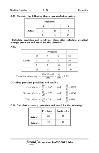
· Conditional self-information is defined as :
I (x |y )
i j = log
1
P (x |y )
log P (x |y ) 0
i j
i j
= - ³
I (x ; y )
i j = log P (x |y ) log P (x )
i j i
-
= I (x ) I (x |y )
i i j
-
· We interpret I (x |y )
i j as the self-information about the event
X xi
= after having observed the event Y = yj.
· The mutual information between a pair of events can be either
positive or negative, or zero since both I (x |y )
i j and I [x ]
i are
greater than or equal to zero.
Q.19 What is entropy ? What are the elements of information
theory ?
Ans. : · Given two random variables, what can we say about one
when we know the other ? This is the central problem in
information theory. Information theory answers two fundamental
questions in communication theory :
1. What is the ultimate lossless data compression ?
2. What is the ultimate transmission rate of reliable
communication ?
· Information theory is more : It gives insight into the problems of
statistical inference, computer science, investments and many
other fields.
· The most fundamental concept of information theory is the
entropy. The entropy of a random variable X is defined by,
H(X) = - å p(x) log p(x)
x
· The entropy measures the expected uncertainty in X. It has the
following properties :
H(X) ³ 0, entropy is always non-negative.
H(X) = 0 iff X is deterministic.
· Since H (X) log (a) H (X)
b b a
= , we don't need to specify the base
of the logarithm.
®

· The entropy is non-negative. It is zero when the random variable
is "certain" to be predicted. Entropy is defined using the Clausius
inequality.
· Entropy is defined in terms of probabilistic behaviour of a source
of information. In information theory the source output are
discrete random variables that have a certain fixed finite alphabet
with certain probabilities.
· Entropy is an average information content for the given source
symbol.
· Entropy (example) : Binary memoryless source has symbols 0 and
1 which have probabilities p0 and p1
(1 – p0). Count the entropy as a function of p0.
· Example : Consider a fair coin toss. There are two outcomes,
each with probability 1/2. The entropy of this random event is,
- +
æ
è
ç
ö
ø
÷
1
2
log
1
2
1
2
log
1
2
2 2 = 1
· This means that the result of the coin flip gives us 1 bit of
information, or that the uncertainty in the outcome of the coin
flip is 1 bit.
· The importance of the entropy, and its use as a measure of
information, derives from the following properties :
1. H 0
x ³
2. Hx = 0 if and only if the random variable X is certain, which
means that X takes one value with probability one.
3. Among all probability distributions on a set X with M
elements, H is maximum when all events x are equi-probable,
with p(x) = 1/M. The entropy is then H log M
x 2
= .
4. If X and Y are two independent random variables, meaning
that p (x, y) p (x) p (y)
X ,Y X Y
= , the total entropy of the pair X,
Y is equal to H H
X Y
+ :
HX, Y = - å p (x, y) log p (x, y)
x, y
2 (X, Y)
®

= - +
å
x, y
X Y 2 X 2 Y
p (x) p (y) (log p (x) log p (y))
= H H
X Y
+
5. For any pair of random variables, one has in general
H H H
X, Y X Y
£ + and this result is immediately generalizable
to n variables.
6. Additivity for composite events. Take a finite set of events X
and decompose it into X X1 X2
= È , where X1 X2
Ç = f. The
total entropy can be written as the sum of two contributions.
HX = å Î
= +
x X 2
p(x) log p(x) H(q) H(r)
where H(q) = q log q q log q
1 2 1 2 2 2
-
H(r) = - -
Î Î
å å
q r (x) log r (x) q r (x) log
1
x X1
1 2 1 2
x X1
2 2 2
r (x)
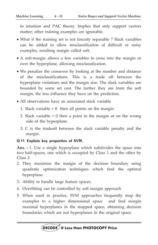
Importance of entropy
1. Entropy is considered one of the most important qualities in
information theory.
2. There exists two types of source coding :
I] Lossless coding II] Lossy coding
3. Entropy is the threshold quantity that separates lossy from
lossless data compression.
END...?
®

2.1 : Scikit - Learn Dataset
Q.1 Define feature selection.
Ans. : Feature selection is a process that chooses a subset of
features from the original features so that the feature space is
Q.2 What is Scikit - learn Dataset? How it helps user to
understand various features ?
Ans. : · Scikit-learn is probably the most useful library for
machine learning in Python. It is on NumPy, SciPy and matplotlib,
this library contains a lot of effiecient tools for machine learning
and statistical modeling including classification, regression,
clustering and dimensionality reduction.
· In scikit-learn, an estimator for classification is a Python object
that implements the methods fit(X, y) and predict(T).
· An example of an estimator is the class sklearn.svm. SVC, which
implements support vector classification. The estimator's
constructor takes as arguments the model's parameters.
· Scikit-learn comes loaded with a lot of features. Here are a few of
them to help you understand :
1. Supervised learning algorithms : Think of any supervised
learning algorithm you might have heard about and there is a
very high chance that it is part of scikit-learn.
®
2 Feature Selection
UNIT - II
(2 - 1)

2. Cross-validation : There are various methods to check the
accuracy of supervised models on unseen data
3. Unsupervised learning algorithms : Again there is a large
spread of algorithms in the offering - starting from clustering,
factor analysis, principal component analysis to unsupervised
neural networks.
4. Various toy datasets : This came in handy while learning
scikit-learn. I had learnt SAS using various academic datasets
(e.g. IRIS dataset, Boston House prices dataset). Having them
handy while learning a new library helped a lot.
5. Feature extraction : Useful for extracting features from images
and text (e.g. Bag of words)
Q.3 How to manage categorical data ?
Ans. : · That categorical data is defined as variables with a finite
set of label values. That most machine learning algorithms require
numerical input and output variables. That an integer and one hot
encoding is used to convert categorical data to integer data.
· Categorical data is very common in business datasets. For
example, users are typically described by country, gender, age
group etc., products are often described by product type,
manufacturer, seller etc., and so on.
· Several regression and binary classification algorithms are
available in scikit-learn. A simple way to extend these algorithms
to the multi-class classification case is to use the so-called
one-vs-all scheme.
· At learning time, this simply consists in learning one regressor or
binary classifier per class. In doing so, one needs to convert
multi-class labels to binary labels. LabelBinarizer makes this
process easy with the transform method.
Machine Learning 2 - 2 Feature Selection
®

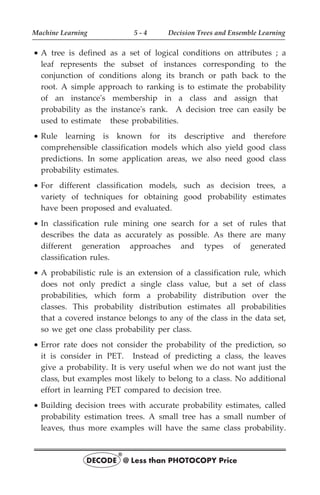
· At prediction time, one assigns the class for which the
corresponding model gave the greatest confidence. LabelBinarizer
makes this easy with the inverse_transform method.
· Example :
>>> from sklearn import preprocessing
>>> lb = preprocessing.LabelBinarizer()
>>> lb.fit([1, 2, 6, 4, 2])
LabelBinarizer(neg_label=0, pos_label=1,sparse_output=False)
>>> lb.classes_
array([1, 2, 4, 6])
>>> lb.transform([1, 6])
array([[1, 0, 0, 0],
[0, 0, 0, 1]])
Q.4 Describe managing missing features.
Ans. : · Sometimes a dataset can contain missing features, so there
are a few options that can be taken into account :
1. Removing the whole line
2. Creating sub-model to predict those features
3. Using an automatic strategy to input them according to the
other known values.
· In real-world samples, it is not uncommon that there are missing
one or more values such as the blank spaces in our data table.
· Quite a few computational tools, however, are unable to handle
such missing values and might produce unpredictable results. So,
before we proceed with further analyses, it is critical that we take
care of those missing values.
· Mean imputation replaces missing values with the mean value of
that feature/variable. Mean imputation is one of the most 'naive'
imputation methods because unlike more complex methods like
k-nearest neighbors imputation, it does not use the information
we have about an observation to estimate a value for it.
®

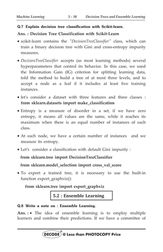
import pandas as pd
import numpy as np
from sklearn.preprocessing import imputer
# Create an empty dataset
df = pd.DataFrame()
# Create two variables called x0 and x1. Make the first value of x1 a
missing value
df['x0'] =
[0.3051,0.4949,0.6974,0.3769,0.2231,0.341,0.4436,0.5897,0.6308,0.5]
df['x1'] =
[np.nan,0.2654,0.2615,0.5846,0.4615,0.8308,0.4962,0.3269,0.5346,0.6731]
# View the dataset
df
x0 x1
0 0.3051 NaN
1 0.4949 0.2654
2 0.6974 0.2615
3 0.3769 0.5846
4 0.2231 0.4615
5 0.3410 0.8308
6 0.4436 0.4962
7 0.5897 0.3269
8 0.6308 0.5346
9 0.5000 0.6731
Fit Imputer
# Create an imputer object that looks for 'Nan' values, then replaces
them with the mean value of the feature by columns (axis=0)
®

mean_imputer = Imputer(missing_values='NaN', strategy='mean',
axis=0)
# Train the imputor on the df dataset
mean_imputer = mean_imputer.fit(df)
Apply Imputer
# Apply the imputer to the df dataset
imputed_df = mean_imputer.transform(df.values)
View Data
# View the data
imputed_df
array([[ 0.3051 , 0.49273333],
[ 0.4949 , 0.2654 ],
[ 0.6974 , 0.2615 ],
[ 0.3769 , 0.5846 ],
[ 0.2231 , 0.4615 ],
[ 0.341 , 0.8308 ],
[ 0.4436 , 0.4962 ],
[ 0.5897 , 0.3269 ],
[ 0.6308 , 0.5346 ],
[ 0.5 , 0.6731 ]])
Notice that 0.49273333 is the imputed value, replacing the np.NaN
value.
Q.5 What is feature selection? Explain role of feature selection in
machine learning. Describe feature selection algorithm.
Ans. : · Feature selection is a process that chooses a subset of
features from the original features so that the feature space is
· Feature selection is a critical step in the feature construction
process. In text categorization problems, some words simply do
not appear very often. Perhaps the word "groovy" appears in
exactly one training document, which is positive. Is it really
worth keeping this word around as a feature? It's a dangerous
endeavor because it's hard to tell with just one training example
if it is really correlated with the positive class, or is it just noise.
®

You could hope that your learning algorithm is smart enough to
figure it out. Or you could just remove it.
· There are three general classes of feature selection algorithms :
filter methods, wrapper methods and embedded methods.
· The role of feature selection in machine learning is
1. to reduce the dimensionality of feature space
2. to speed up a learning algorithm
3. to improve the predictive accuracy of a classification algorithm
4. to improve the comprehensibility of the learning results
· Features Selection Algorithms are as follows :
1. Instancebased approaches : There is no explicit procedure for
feature subset generation. Many small data samples are
sampled from the data. Features are weighted according to
their roles in differentiating instances of different classes for a
data sample. Features with higher weights can be selected.
2. Nondeterministic approaches : Genetic algorithms and
simulated annealing are also used in feature selection.
3. Exhaustive complete approaches : Branch and Bound
evaluates estimated accuracy and ABB checks an inconsistency
measure that is monotonic. Both start with a full feature set
until the preset bound cannot be maintained.
Q.6 Discuss feature selection classes SelectKBest and
SelectPercentile.
Ans. : · Two examples of feature selection that use the classes
SelectKBest and SelectPercentile.
· The classes in the sklearn.feature_selection module can be used
for feature selection/dimensionality reduction on sample sets,
either to improve estimators' accuracy scores or to boost their
performance on very high-dimensional datasets.
· VarianceThreshold is a simple baseline approach to feature
selection. It removes all features whose variance doesn't meet
®

some threshold. By default, it removes all zero-variance features,
i.e. features that have the same value in all samples.
· As an example, suppose that we have a dataset with boolean
features, and we want to remove all features that are either one
or zero (on or off) in more than 80% of the samples.
· Boolean features are Bernoulli random variables, and the variance
of such variables is given by Var[X] = p(1 – p)
>>> from sklearn.feature_selection import VarianceThreshold
>>> X = [[0, 0, 1], [0, 1, 0], [1, 0, 0], [0, 1, 1], [0, 1, 0], [0, 1, 1]]
>>> sel = VarianceThreshold(threshold=(.8 * (1 - .8)))
>>> sel.fit_transform(X)
array([[0, 1],
[1, 0],
[0, 0],
[1, 1],
[1, 0],
[1, 1]])
· Univariate feature selection works by selecting the best features
based on univariate statistical tests. It can be seen as a
preprocessing step to an estimator. Scikit-learn exposes feature
selection routines as objects that implement the transform
method :
1. SelectKBest removes all but the k highest scoring features.
2. SelectPercentile removes all but a user-specified highest scoring
percentage of features.
3. Using common univariate statistical tests for each feature :
false positive rate SelectFpr, false discovery rate SelectFdr or
family wise error SelectFwe.
4. GenericUnivariateSelect allows to perform univariate feature
selection with a configurable strategy. This allows to select the
best univariate selection strategy with hyper-parameter search
estimator.
®

2.2 : Principle Component Analysis (PCA)
Q.7 What is Nonnegative Matrix Factorization? How does it work?
Ans. : Non Negative Matrix Factorization (NMF)
· Nonnegative Matrix Factorization is a matrix factorization method
where we constrain the matrices to be nonnegative. In order to
understand NMF, we should clarify the underlying intuition
between matrix factorization.
· Suppose we factorize a matrix X into two matrices W and H so
that X = W H.
· There is no guarantee that we can recover the original matrix, so
we will approximate it as best as we can.
· Now, suppose that X is composed of m rows, x1, x2 , … xm, W is
composed of k rows w1, w2 , … wk , H is composed of m rows
h1, h2 , … hm.
· Each row in X can be considered a data point. For instance, in
the case of decomposing images, each row in X is a single image,
and each column represents some feature,
X =
x
x
x
1
2
k
L
é
ë
ê
ê
ê
ê
ù
û
ú
ú
ú
ú
, W =
w
w
w
1
2
k
L
é
ë
ê
ê
ê
ê
ù
û
ú
ú
ú
ú
, H =
h
h
h
1
2
k
L
é
ë
ê
ê
ê
ê
ù
û
ú
ú
ú
ú
· Take the ith row in X, xi . If you think about the equation, you
will find that xi can be written as
xi = w h
ij i
j 1
k
´
=
å
· Basically, we can interpret xi to be a weighted sum of some
components, where each row in H is a component, and each row
in W contains the weights of each component.
®

How Does it Work ?
· NMF decomposes multivariate data by creating a user-defined
number of features. Each feature is a linear combination of the
original attribute set; the coefficients of these linear combinations
are non-negative.
· NMF decomposes a data matrix V into the product of two lower
rank matrices W and H so that V is approximately equal to W
times H.
· NMF uses an iterative procedure to modify the initial values of
W and H so that the product approaches V. The procedure
terminates when the approximation error converges or the
specified number of iterations is reached.
· During model apply, an NMF model maps the original data into
the new set of attributes (features) discovered by the model.
Q.8 Explain difference between PCA and NMF.
Ans. :
Sr. No. PCA NMF
1. It uses unsupervised
dimensionality reduction.
It also uses unsupervised
2. Orthogonal vectors with
positive and negative
coefficients.
Non-negative coefficients.
3. Difficult to interpret. Easier to interpret.
4. PCA is non-iterative. NMF is iterative.
5. Designed for producing
optimal basis images.
Designed for producing
coefficients with a specific
property.
®

Q.9 Write short note on following :
a. Sparse PCA b. Kernel PCA
Ans. : a. Sparse PCA : · In sparse PCA one wants to get a small
number of features which still capture most of the variance. Thus
one needs to enforce sparsity of the PCA component, which yields
a trade-off between explained variance and sparsity.
· To address the non-sparsity issue of traditional PCA, sparse PCA
imposes additional constraint on the number of non-zero element
in the vector v.
· This is achieved through the l 0
norm, which gives the number of
non-zero element in the vector v. A sparse PCA with at most k
non-zero loadings can then be formulated as the following
optimization problem.
· Optimization problems with l 0 norm constraint is in general
NP-hard. Therefore, most methods for sparse PCA relaxes the l 0
norm constraint with l 1
norm appended to the objective function.
b. Kernel PCA : · Kernel PCA is the nonlinear form of PCA, which
better exploits the complicated spatial structure of high-dimensional
features.
· It can extract up to n (number of samples) nonlinear principal
components without expensive computations.
· The standard steps of kernel PCA dimensionality reduction can
be summarized as :
1. Construct the kernel matrix K from the training data set
2. Compute the gram matrix
3. Solve N-dimensional column vector
4. Compute the kernel principal components
· Kernel PCA supports both transform and inverse_transform.
· Fig. Q.9.1 (a), (b) shows PCA and KPCA.
®

Preliminaries :
# Load libraries
from sklearn.decomposition import PCA, KernelPCA
from sklearn.datasets import make_circles
Create Linearly Inseparable Data :
# Create linearly inseparable data
X, _ = make_circles(n_samples=1000, random_state=1, noise=0.1,
factor=0.1)
®
×
×
×
×
×
× ××
×
×
×
× ×
×
×
× ×
×
×
×
×
×
×
×
×
× ×
×
×
×
×××
×
×
×
×
×
×
× ×
×
×
×
×
×
×××
×
×
×
×
× ×
×
×
×
× × ×
××
× ×
×
×
×
×
×
×
× × ×
×
×
×
×
×
×
×
×
×
×
×
×
×
××
×
×
× ×
×
× ×
×
×
×
×
×
×
×
×
×
×
× ×
×
×
××
×
× × × ××
××× × ×
×
×
×
× ×
×××
×
×
×
×
××
×
×
×
×
×
× ×
× ×
×
×
×
×
×
× × × ×
×
×
× × ×× ×
×
×
×
×
× ×
×××
×
×
×
×
× ×
×
×
×
×
×
×
×
×
××
× ×
×
×
× × ×
×
×
×××
×
×
×
×
×
×
× × × ×
×
×
×
× ×
××
×
×
×
×
×
×
×
×
×× ×
×
××
×
×
×
×
× ×
×
×
×
×
× ×
×
×
×
×
×
×
× ××
×
××
×
×
××
×
×
×
×
×
×
××
× ×
×
×
× ×
×
×
×
××××
×
×
×
× ××
×
×
×
×
×
× ×
× ×
×
×
×
×
×
××
×
×
×
×
×
×
×
××
×
×
×
×
××
××
×
×
–0.8 –0.6 –0.4 –0.2 0 0.2 0.4 0.6
0.8
0.6
0.4
0.2
0
–0.2
–0.4
–0.6
x
2
x1
0.6
(a) : PCA
×
×
×
×
×
× ××
×
×
×
× ×
×
×
× ×
×
×
×
×
×
×
×
×
× ×
×
×
×
×××
×
×
×
×
×
×
× ×
×
×
×
×
×
×××
×
×
×
×
× ×
×
×
×
× × ×
××
× ×
×
×
×
×
×
×
× × ×
×
×
×
×
×
×
×
×
×
×
×
×
×
××
×
×
× ×
×
× ×
×
×
×
×
×
×
×
×
×
×
× ×
×
×
××
×
× × × ××
××× × ×
×
×
×
× ×
××
×
×
×
×
×
××
×
×
×
×
× × ×
× ×
×
×
×
×
×
× × × ×
×
×
× × ×× ×
×
×
×
×
× ×
×××
×
×
×
×
× ×
×
×
×
×
×
×
×
×
××
× ×
×
×
× × ×
×
×
×××
×
×
×
×
×
×
× × × ×
×
×
×
× ×
××
×
×
×
×
×
×
×
×
×× ×
×
××
×
×
×
×
× ×
×
×
×
×
× ×
×
×
×
×
×
×
×
×
×
×
××
×
×
××
×
×
×
×
×
×
××
× ×
× ×
×
×
×
××××
×
×
×
× ××
×
×
×
×
×
× ×
× ×
×
×
×
×
× ××
××
×
×
×
×
×
××
×
×
×
×
××
××
×
×
–0.8 –0.6 –0.4 –0.2 0 0.2 0.4 0.6 0.8
0.8
0.6
0.4
0.2
0
–0.2
–0.4
–0.6
x2
x1
(b) : KPCA
Fig. Q.9.1

Conduct Kernel PCA :
# Apply kernal PCA with radius basis function (RBF) kernel
kpca = KernelPCA(kernel="rbf", gamma=15, n_components=1)
X_kpca = kpca.fit_transform(X)
2.3 : Atom Extraction and Dictionary Learning
Q.10 Write short note on Atom Extraction and Dictionary Learning.
Ans. : Atom Extraction and Dictionary Learning
· Dictionary learning is a technique which allows rebuilding a
sample starting from a sparse dictionary of atoms.
· A dictionary can be good for representing a class of signals, but
not for representing white Gaussian noise.
· In scikit-learn, we can implement such an algorithm with the
class DictionaryLearning, where n_components, as usual,
determines the number of atoms :
from sklearn.decomposition import DictionaryLearning
>>> dl = DictionaryLearning(n_components=36,
fit_algorithm='lars', transform_algorithm='lasso_lars')
>>> X_dict = dl.fit_transform(digits.data)
· The SparseCoder object is an estimator that can be used to
transform signals into sparse linear combination of atoms from a
fixed, precomputed dictionary such as a discrete wavelet basis.
· This object therefore does not implement a fit method. The
transformation amounts to a sparse coding problem: finding a
representation of the data as a linear combination of as few
dictionary atoms as possible.
· All variations of dictionary learning implement the following
transform methods, controllable via the transform_method
initialization parameter :
1. Orthogonal matching pursuit (Orthogonal Matching Pursuit
(OMP))
®

2. Least-angle regression (Least Angle Regression)
3. Lasso computed by least-angle regression
4. Lasso using coordinate descent (Lasso)
5. Thresholding.
· The dictionary learning objects offer, via the split_code parameter,
the possibility to separate the positive and negative values in the
results of sparse coding.
· This is useful when dictionary learning is used for extracting
features that will be used for supervised learning, because it
allows the learning algorithm to assign different weights to
negative loadings of a particular atom, from to the corresponding
positive loading.
END...?
®

3.1 Linear Regression
Q.1 Define and explain regression with its model.
Ans. : · For an input x, if the output is continuous, this is called a
regression problem. For example, based on historical information of
demand for tooth paste in your supermarket, you are asked to
predict the demand for the next month.
· Regression is concerned with the prediction of continuous
quantities. Linear regression is the oldest and most widely used
predictive model in the field of machine learning. The goal is to
minimize the sum of the squared errors to fit a straight line to a
set of data points.
· For regression tasks, the typical accuracy metrics are Root Mean
Square Error (RMSE) and Mean Absolute Percentage Error
(MAPE). These metrics measure the distance between the
predicted numeric target and the actual numeric answer.
Regression Line
· Least squares : The least squares regression line is the line that
makes the sum of squared residuals as small as possible. Linear
means "straight line".
· Regression line is the line which gives the best estimate of one
variable from the value of any other given variable.
· The regression line gives the average relationship between the
two variables in mathematical form.
· For two variables X and Y, there are always two lines of
regression.
®
3 Regression
UNIT - III
(3 - 1)

· Regression line of X on Y gives the best estimate for the value of
X for any specific given values of Y :
X = a + b Y
where a = X - intercept
b = Slope of the line
X = Dependent variable
Y = Independent variable
· Regression line of Y on X : gives the best estimate for the value
of Y for any specific given values of X :
Y = a + bx
where
a = Y - intercept
b = Slope of the line
Y = Dependent variable
x = Independent variable
· By using the least squares method (a procedure that minimizes
the vertical deviations of plotted points surrounding a straight
line) we are able to construct a best fitting straight line to the
scatter diagram points and then formulate a regression equation
in the form of :
$
y = a + bX
$
y = y b (x x)
+ -
Machine Learning 3 - 2 Regression
®
Y
b = Slope
Change
in Y
a = Y - intercept
X
y =
a +
bX
^
Change in X
Y = + X +
i 0 1 i i
Dependent
variable
Independent
variable
Population
y - intercept
Population
slope Random
error
Fig. Q.1.1 Regression

· Regression analysis is the art and science of fitting straight lines
to patterns of data. In a linear regression model, the variable of
interest ("dependent" variable) is predicted from k other variables
("independent" variables) using a linear equation. If Y denotes the
dependent variable, and X , ..., X
1 k, are the independent variables,
then the assumption is that the value of Y at time t in the data
sample is determined by the linear equation :
Y1 = b b b b e
0 1 1t 2 2t k kt t
X X ... X
+ + + + +
where the betas are constants and the epsilons are independent and
identically distributed normal random variables with mean zero.
· In a regression tree the idea is this : since the target variable does
not have classes, we fit a regression model to the target variable
using each of the independent variables. Then for each
independent variable, the data is split at several split points.
· At each split point, the "error" between the predicted value and
the actual values is squared to get a "Sum of Squared Errors
(SSE)". The split point errors across the variables are compared
and the variable/point yielding the lowest SSE is chosen as the
root node/split point. This process is recursively continued.
· Error function measures how much our predictions deviate from
the desired answers.
Mean-squared error Jn =
1
n
(y f (x ))
i 1 ... n
i i
2
=
å -
· Multiple linear regression is an extension of linear regression,
which allows a response variable, y, to be modeled as a linear
function of two or more predictor variables
®
f (x,w)
w0
w1
w2
wd
1
x1
x2
xd
Bias term
Input vector
X
Fig. Q.1.2

Evaluating a Regression Model
· Assume we want to predict a car's price using some features
such as dimensions, horsepower, engine specification, mileage etc.
This is a typical regression problem, where the target variable
(price) is a continuous numeric value.
· We can fit a simple linear regression model that, given the
feature values of a certain car, can predict the price of that car.
This regression model can be used to score the same dataset we
trained on. Once we have the predicted prices for all of the cars,
we can evaluate the performance of the model by looking at how
much the predictions deviate from the actual prices on average
Advantages :
a. Training a linear regression model is usually much faster than
methods such as neural networks.
b. Linear regression models are simple and require minimum
memory to implement.
c. By examining the magnitude and sign of the regression
coefficients you can infer how predictor variables affect the
target outcome.
Q.2 When is it suitable to use linear regression over
classification ?
Ans. : · Linear regression is a statistical method that allows us to
summarize and study relationships between two continuous
(quantitative) variables :
1. One variable, denoted x, is regarded as the predictor,
explanatory, or independent variable.
2. The other variable, denoted y, is regarded as the response,
outcome, or dependent variable.
· Regression models predict a continuous variable, such as the
sales made on a day or predict temperature of a city.
· Let's imagine that you fit a line with the training points you
have. Imagine you want to add another data point, but to fit it,
®

you need to change your existing model (maybe the threshold
itself, as well).
· This will happen with each data point that we add to the model;
hence, linear regression isn't good for classification models.
· Regression estimates are used to explain the relationship between
one dependent variable and one or more independent variables.
n Classification predicts categorical labels (classes), prediction
models continuous - valued functions. Classification is
considered to be supervised learning.
n Classifies data based on the training set and the values in a
classifying attribute and uses it in classifying new data.
Prediction means models continuous - valued functions, i.e.
predicts unknown or missing values.
Q.3 What are the limitations of linear regression ? How it is
overcome by using higher dimensionality ?
Ans. : · There are two important shortcomings of linear
regression :
1. Predictive ability : The linear regression fit often has low bias
but high variance. Recall that expected test error is a
combination of these two quantities. Prediction accuracy can
sometimes be improved by sacrificing some small amount of
bias in order to decrease the variance.
2. Interpretative ability : Linear regression freely assigns a
coefficient to each predictor variable. When the number of
variables p is large, we may sometimes seek, for the sake of
interpretation, a smaller set of important variables.
· These shortcomings become major problems in a
high-dimensional regression setting, where the number of
predictors p rivals or even exceeds the number of observations n.
In fact, when p > n, the linear regression estimate is actually not
well-defined.
· scikit-learn offers the class linear regression, which works with
n-dimensional spaces.
®

· For example, take boston data from dummy sklearn datasets :
from sklearn.datasets import load_boston
boston = load_boston()
X, y = boston.data, boston.target
· We split the original dataset into training (90 %) and test (10 %)
sets :
from sklearn.linear_model import LinearRegression
from sklearn.model_selection import train_test_split
· When the original data set isn't large enough, splitting it into
training and test sets may reduce the number of samples that can
be used for fitting the model.
· The k-fold cross-validation can help in solving this problem with
a different strategy.
· The whole dataset is split into k folds using always k-1 folds for
training and the remaining one to validate the model. K iterations
will be performed, using always a different validation fold.
Q.4 Explain least square method.
Ans. : · The method of least squares is about estimating parameters
by minimizing the squared discrepancies between observed data,
on the one hand, and their expected values on the other.
· Considering an arbitrary straight line, y = b b x
0 1
+ , is to be fitted
through these data points. The question is "Which line is the
most representative" ?
· What are the values of b and b
0 1 such that the resulting line
"best" fits the data points ? But, what goodness-of-fit criterion to
use to determine among all possible combinations of b and b
0 1 ?
· The Least Squares (LS) criterion states that the sum of the
squares of errors is minimum. The least-squares solutions yields
y(x) whose elements sum to 1, but do not ensure the outputs to
be in the range [0,1].
®

· How to draw such a line based on data points observed ?
Suppose a imaginary line of y = a + bx.
· Imagine a vertical distance between the line and a data point
E = Y – E(Y).
· This error is the deviation of the data point from the imaginary
line, regression line. Then what is the best values of a and b ? a
and b that minimizes the sum of such errors.
®
Xi
0
yi
^
yi
e = y – ^
y =Error (residual)
i i i
1
1
^
y = 0 1x
y
x
Fig. Q.4.1
4
3
2
1
0
3
2
1
0 4 5
x1
e1
E(Y)=a + b X
x3
e3
e2
x2
y
x
Fig. Q.4.2

· Deviation does not have good properties for computation. Then
why do we use squares of deviation ? Let us get a and b that can
minimize the sum of squared deviations rather than the sum of
deviations. This method is called least squares.
· Least squares method minimizes the sum of squares of errors.
Such a and b are called least squares estimators i.e. estimators of
parameters a and b.
· The process of getting parameter estimators (e.g., a and b) is
called estimation. Lest squares method is the estimation method
of Ordinary Least Squares (OLS).
Disadvantages of least square
1. Lack robustness to outliers
2. Certain datasets unsuitable for least squares classification
3. Decision boundary corresponds to ML solution
3.2 Ridge, Lasso and ElasticNet
Q.5 Write short note on ElasticNet.
Ans. : · ElasticNet, which combines both Lasso and Ridge into a
single model with two penalty factors : One proportional to L1
norm and the other to L2 norm.
· Elastic net is a related technique. Use elastic net when you have
several highly correlated variables. Lasso provides elastic net
regularization when you set the alpha name-value pair to a
number strictly between 0 and 1.
· Elastic net can generate reduced models by generating
zero-valued coefficients. Empirical studies have suggested that the
elastic net technique can outperform lasso on data with highly
correlated predictors.
· The elastic net technique solves this regularization problem. For
an a strictly between 0 and 1 and a nonnegative l, elastic net
solves the problem.
®

· The ElasticNet loss function is defined as :
L(w) =
1
2n
|
|Xw – y|| ||w|| +
(1– )
2
||w||
2
2
1 2
2
+ab
a b
· The ElasticNet class provides an implementation where the alpha
parameter works in conjunction with l1_ratio. The main
peculiarity of ElasticNet is avoiding a selective exclusion of
correlated features, thanks to the balanced action of the L1 and
L2 norms.
Q.6 What is ride regression and lasso ?
Ans. : · Ridge regression and the Lasso are two forms of
regularized regression. These methods are seeking to improve the
consequences of multicollinearity.
1. When variables are highly correlated, a large coefficient in one
variable may be alleviated by a large coefficient in another
variable, which is negatively correlated to the former.
2. Regularization imposes an upper threshold on the values taken
by the coefficients, thereby producing a more parsimonious
solution, and a set of coefficients with smaller variance.
· Ridge estimation produces a biased estimator of the true
parameter b.
E |X]
ridge
[$
b = (X X+ I) X X
T – 1 T
l b
= (X X+ I) X X+ I – I)
T – 1 T
l l l b
(
= [I – (X X+ I) ]
T – 1
l l b
= b l l b
– (X X+ I)
T – 1
· Ridge regression shrinks the regression coefficients by imposing a
penalty on their size. The ridge coefficients minimize a penalized
residual sum of squares.
· Ridge regression protects against the potentially high variance of
gradients estimated in the short directions.
Lasso
· One significant problem of ridge regression is that the penalty
term will never force any of the coefficients to be exactly zero.
®

Thus, the final model will include all p predictors, which creates
a challenge in model interpretation. A more modern machine
learning alternative is the lasso.
· The lasso works in a similar way to ridge regression, except it
uses a different penalty term that shrinks some of the coefficients
exactly to zero.
· Lasso : Lasso is a regularized regression machine learning
technique that avoids over-fitting of training data and is useful
for feature selection.
· The lasso is a shrinkage method like ridge, with subtle but
important differences. The lasso estimate is defined by,
$
blasso = argmin
b
b b
y – – x
i 0 j ij
j= 1
p
i= 0
n
å
å
æ
è
ç
ç
ö
ø
÷
÷
2
subject to bj
j= 1
p
å < t
· Note the name “lasso" is actually an acronym for : Least
Absolute Selection and Shrinkage Operator.
· The only difference from Ridge regression is that the
regularization term is in absolute value. But this difference has a
huge impact on the trade-off.
· Lasso method overcomes the disadvantage of Ridge regression by
not only punishing high values of the coefficients b but actually
setting them to zero if they are not relevant.
Q.7 Explain the difference between ridge regression and lasso.
Ans. :
1. The lasso has a major advantage over ridge regression, in that it
produces simpler and more interpretable models that involved
only a subset of predictors.
2. The lasso leads to qualitatively similar behavior to ridge
regression, in that as l increases, the variance decreases and the
bias increases.
®

3. The lasso can generate more accurate predictions compared to
ridge regression.
4. Cross-validation can be used in order to determine which
approach is better on a particular data set.
Q.8 What is random sample consensus ? How it achieves the
goals.
Ans. : · Random sample consensus (RANSAC) is an iterative
method to estimate parameters of a mathematical model from a set
of observed data that contains outliers, when outliers are to be
accorded no influence on the values of the estimates. Therefore, it
also can be interpreted as an outlier detection method.
· It is a non-deterministic algorithm in the sense that it produces a
reasonable result only with a certain probability, with this
probability increasing as more iterations are allowed.
· RANSAC divides data into inliers and outliers and yields
estimate computed from minimal set of inliers with greatest
support.
· Improve this initial estimate with Least Squares estimation over
all inliers (i.e., standard minimization). Find inliers w.r.t that L.S.
line and compute L.S. one more time.
· The RANSAC algorithm is essentially composed of two steps that
are iteratively repeated :
1. In the first step, a sample subset containing minimal data
items is randomly selected from the input dataset. A fitting
model and the corresponding model parameters are computed
using only the elements of this sample subset. The cardinality
of the sample subset is the smallest sufficient to determine the
model parameters.
®
A
B
C
D
A
B
C D
Fig. Q.8.1

2. In the second step, the algorithm checks which elements of the
entire dataset are consistent with the model instantiated by the
estimated model parameters obtained from the first step. A
data element will be considered as an outlier if it does not fit
the fitting model instantiated by the set of estimated model
parameters within some error threshold that defines the
maximum deviation attributable to the effect of noise.
· The input to the RANSAC algorithm is a set of observed data
values a way of fitting some kind of model to the observations,
and some confidence parameters. RANSAC achieves its goal by
repeating the following steps :
1. Select a random subset of the original data. Call this subset the
hypothetical inliers.
2. A model is fitted to the set of hypothetical inliers.
3. All other data are then tested against the fitted model. Those
points that fit the estimated model well, according to some
model-specific loss function, are considered as part of the
consensus set.
4. The estimated model is reasonably good if sufficiently many
points have been classified as part of the consensus set.
5. Afterwards, the model may be improved by re-estimating it
using all members of the consensus set.
3.3 Polynomial Regression and Logistic Regression
Q.9 What is perceptron ? Define the architecture of a perceptron ?
What do you mean by linear separability ?
Ans. : · The perceptron is a feed - forward network with one
output neuron that learns a separating hyper - plane in a pattern
space.
· The "n" linear Fx neurons feed forward to one threshold output
Fy neuron. The perceptron separates linearly separable set of
patterns.
®

Architecture of a perceptron :
· The perceptron is a feed-forward network with one output
neuron that learns a separating hyper-plane in a pattern space.
The "n" linear Fx neurons feed forward to one threshold output
patterns.
· SLP is the simplest type of artificial neural networks and can
only classify linearly separable cases with a binary target (1 , 0).
· We can connect any number of McCulloch-Pitts neurons together
in any way we like. An arrangement of one input layer of
McCulloch-Pitts neurons feeding forward to one output layer of
McCulloch-Pitts neurons is known as a Perceptron.
· A single layer feed-forward network consists of one or more
output neurons, each of which is connected with a weighting
factor Wij to all of the inputs Xi .
· The Perceptron is a kind of a single-layer artificial network with
only one neuron. The Percepton is a network in which the
neuron unit calculates the linear combination of its real-valued or
boolean inputs and passes it through a threshold activation
function. Fig. Q.9.1 shows Perceptron.
®
Weight
W1
Weight
W2
Weight
WN
S
Input 1
Input 2
Input N
·
·
·
Threshold
Output
Sigmoid
Fig. Q.9.1

· The Perceptron is sometimes referred to a Threshold Logic Unit
(TLU) since it discriminates the data depending on whether the
sum is greater than the threshold value.
· In the simplest case the network has only two inputs and a single
output. The output of the neuron is :
y = f W X b
i 1
2
i i
=
å +
æ
è
ç
ç
ö
ø
÷
÷
· Suppose that the activation function is a threshold then
f =
1 if s 0
1 if s 0
>
- £
ì
í
î
· The Perceptron can represent most of the primitive boolean
functions : AND, OR, NAND and NOR but can not represent
XOR.
· In single layer perceptron, initial weight values are assigned
randomly because it does not have previous knowledge. It sum
all the weighted inputs. If the sum is greater than the threshold
value then it is activated i.e. output = 1.
Output
W X W X ... W X
1 1 2 2 n n
+ + + > q Þ 1
W X W X ... W X
1 1 2 2 n n
+ + + £ q Þ 0
· The input values are presented to the perceptron, and if the
predicted output is the same as the desired output, then the
performance is considered satisfactory and no changes to the
weights are made.
· If the output does not match the desired output, then the weights
need to be changed to reduce the error.
· The weight adjustment is done as follows :
DW = h d x
´ ´
Where X = Input data
®

d = Predicted output and desired output.
h = Learning rate
· If the output of the perceptron is correct then we do not take any
action. If the output is incorrect then the weight vector is
W W W
® + D .
· The process of weight adaptation is called learning.
· Perceptron Learning Algorithm :
1. Select random sample from training set as input.
2. If classification is correct, do nothing.
3. If classification is incorrect, modify the weight vector W using
Wi = W d (n) X (n)
i i
+h
Repeat this procedure until the entire training set is classified
correctly.
Q.10 What do you mean by linear separability ?
Ans. : Linear separable problem
· Consider two-input patterns (x ,x )
1 2 being classified into two
classes as shown in Fig. Q.10.1. Each point with either symbol of
x or 0 represents a pattern with a set of values (x ,x )
1 2 .
· Linearly separable sets : There
exist a hyperplane (here a
line) that correctly classifies
all points.
· Each pattern is classified into
one of two classes. Notice that
these classes can be separated
with a single line L. They are
known as linearly separable
patterns.
®
x1
x2
Fig. Q.10.1 Two class

· Linear separability refers to the fact that classes of patterns with
n-dimensional vector x = (x1, x2 ,…, xn ) can be separated with a
single decision surface. In the case above, the line L represents
the decision surface.
· If two classes of patterns can be separated by a decision
boundary, represented by the linear equation then they are said
to be linearly separable. The simple network can correctly classify
any patterns.
· Decision boundary of linearly separable classes can be
determined either by some learning procedures or by solving
linear equation systems based on representative patterns of each
class.
· If such a decision boundary does not exist, then the two classes
are said to be linearly inseparable.
· Linearly inseparable problems cannot be solved by the simple
network, more sophisticated architecture is needed.
Q.11 What is logistic regression ? How it outperforms basic linear
classifier ?
Ans. : · Logistic regression is a form of regression analysis in
which the outcome variable is binary or dichotomous. A statistical
method used to model dichotomous or binary outcomes using
predictor variables.
· Logistic component : Instead of modeling the outcome, Y,
directly, the method models the log odds (Y) using the logistic
function.
· Regression component : Methods used to quantify association
between an outcome and predictor variables. It could be used to
build predictive models as a function of predictors.
· In simple logistic regression, logistic regression with 1 predictor
variable.
®

Logistic Regression :
ln
P(Y)
1 – P(Y)
æ
è
ç
ö
ø
÷ = b b b b
0 1 2
+ + + +
X X X
1 2 k k
...
Y = b b b b e
0 1 2
+ + + + +
X X X
1 2 k k
...
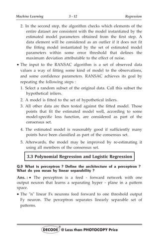
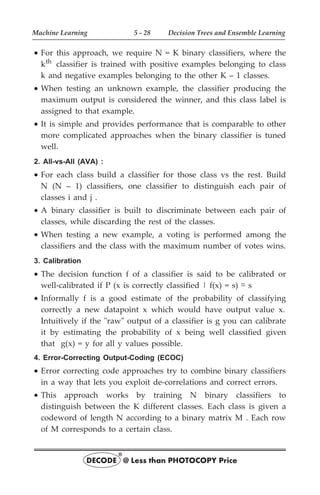
· With logistic regression, the response variable is an indicator of
some characteristic, that is, a 0/1 variable. Logistic regression is
used to determine whether other measurements are related to the
presence of some characteristic, for example, whether certain
blood measures are predictive of having a disease.
· If analysis of covariance can be said to be a t test adjusted for
other variables, then logistic regression can be thought of as a
chi-square test for homogeneity of
proportions adjusted for other
variables. While the response
variable in a logistic regression is a
0/1 variable, the logistic regression
equation, which is a linear
equation, does not predict the 0/1
variable itself.
· Fig. Q.11.1 shows Sigmoid curve
for logistic regression.
· The linear and logistic probability models are :
Linear Regression :
p = a a X a X a X
1 2 k k
0 1 2
+ + + +
...
Logistic Regression :
ln[ ]
p (1 – p) = b b X b X b X
1 2 k k
0 1 2
+ + + +
...
· The linear model assumes that the probability p is a linear
function of the regressors, while the logistic model assumes that
the natural log of the odds p/(1 – p) is a linear function of the
regressors.
· The major advantage of the linear model is its interpretability. In
the linear model, if a 1 is 0.05, that means that a one-unit
increase in X1 is associated with a 5 % point increase in the
probability that Y is 1.
®
Linear
Logistic
1.0
0.0
X
Fig. Q.11.1

· The logistic model is less interpretable. In the logistic model, if
b1 is 0.05, that means that a one - unit increase in X1 is
associated with a 0.05 increase in the log odds that Y is 1. And
what does that mean ? I’ve never met anyone with any intuition
for log odds.
Q.12 How scikit-learn implements the logistic regression ?
Ans. : · scikit-learn implements the "LogisticRegression" class,
which can solve problem using optimized algorithms.
· For example, the sklearn.linear_model.LinearRegression estimator
allows the user to specify whether or not to fit an intercept term.
This is done by setting the corresponding constructor arguments
of the estimator object.
· In order to immediately test the accuracy of our classification, it's
useful to split the dataset into training and test sets : from
sklearn.model_selection import train_test_split
· Now we can train the model using the default parameters :
from sklearn.linear_model import LogisticRegression
· It's also possible to check the quality through a cross-validation :
from sklearn.model_selection import cross_val_score.
· Optimization in machine learning has a slight difference.
Generally, while optimizing, we know exactly how our data looks
like and what areas we want to improve. But in machine learning
we have no clue how our "new data" looks like, let alone try to
optimize on it.
· So in machine learning, we perform optimization on the training
data and check its performance on a new validation data.
3.4 Stochastic Gradient Descendent Algorithms
Q.13 What is stochastic gradient descent ?
Ans. : · Much of machine learning can be written as an
optimization problem.
®

· Example loss functions : Logistic regression, linear regression,
principle component analysis, neural network loss.
· A very efficient way to train logistic models is with Stochastic
Gradient Descent (SGD).
· One challenge with training on power law data
(i.e. most data) is that the terms in the gradient can have very
different strengths
· The idea behind stochastic gradient descent is iterating a weight
update based on the gradient of loss function :
w(k + 1) = w(k)– L(w)
g Ñ
· Logistic regression is designed as a binary classifer (output say
{0, 1}) but actually outputs the probability that the input instance
is in the "1" class.
· A logistic classifier has the form :
p(X) =
1
1+ exp(– X )
b
where X = (X1,…, Xn ) is a vector of features.
· Stochastic gradient has some serious limitations however,
especially if the gradients vary widely in magnitude. Some
coefficients change very fast, others very slowly.
· This happens for text, user activity and social media data (and
other power-law data), because gradient magnitudes scale with
feature frequency, i.e. over several orders of magnitude.
· It is not possible to set a single learning rate that trains the
frequent and infrequent features at the same time.
· An example of stochastic gradient descent with perceptron loss
is shown as follows :
from sklearn.linear_model import SGDClassifier
Q.14 How to find optimal hyper-parameters through grid search ?
Ans. : · In statistics, hyperparameter is a parameter from a prior
distribution; it captures the prior belief before data is observed.
®

· In any machine learning algorithm, these parameters need to be
initialized before training a model.
· Model hyperparameters are the properties that govern the entire
training process
· Hyperparameters are important because they directly control the
behaviour of the training algorithm and have a significant impact
on the performance of the model is being trained.
· Choosing appropriate hyperparameters plays a crucial role in the
success of our neural network architecture. Since it makes a huge
impact on the learned model.
· For example, if the learning rate is too low, the model will miss
the important patterns in the data. If it is high, it may have
collisions.
· Choosing good hyperparameters gives two benefits :
1. Efficiently search the space of possible hyperparameters.
2. Easy to manage a large set of experiments for hyperparameter
tuning.
· The process of finding most optimal hyperparameters in
machine learning is called hyperparameter optimisation.
· Grid search is a very traditional technique for implementing
hyperparameters. It brute force all combinations. Grid search
requires to create two set of hyperparameters.
1. Learning rate
2. Number of layers
· Grid search trains the algorithm for all combinations by using the
two set of hyperparameters and measures the performance using
"Cross Validation" technique.
· This validation technique gives assurance that our trained model
got most of the patterns from the dataset.
®

· One of the best methods to do validation by using "K-Fold Cross
Validation" which helps to provide ample data for training the
model and ample data for validations.
· With this technique, we simply build a model for each possible
combination of all of the hyperparameter values provided,
evaluating each model and selecting the architecture which
produces the best results.
· For example, say you have two continuous parameters a and b,
where manually selected values for the parameters are the
following :
a Î {0, 1, 2}
b Î {.25, .50, .75}
· Then the pairing of the selected hyperparametric values, H, can
take on any of the following :
H Î {(0, .25), (0, .50), (0, .75), (1, .25), (1, .50), (1, .75), (2, .25), (2, .50),
(2, .75)}
· Grid search will examine each pairing of a and b to determine
the best performing combination. The resulting pairs, H, are
simply each output that results from taking the Cartesian product
of a and b.
· While straightforward, this "brute force" approach for
hyperparameter optimization has some drawbacks.
Higher-dimensional hyperparametric spaces are far more time
consuming to test than the simple two-dimensional problem
presented here.
· Also, because there will always be a fixed number of training
samples for any given model, the model's predictive power will
decrease as the number of dimensions increases. This is known as
Hughes phenomenon.
®

3.5 Classification Metric
Q.15 Explain binary classification performance evaluation
parameters.
Ans. : · Performance metrics for binary classification are designed
to capture tradeoffs between four fundamental population
quantities : true positives, false positives, true negatives and false
negatives.
· The evaluation measures in classification problems are defined
from a matrix with the numbers of examples correctly and
incorrectly classified for each class, named confusion matrix.
· The confusion matrix for a binary classification problem is shown
below.
· A confusion matrix contains information about actual and
predicted classifications done by a classification system.
Performance of such systems is commonly evaluated using the
data in the matrix. Confusion matrix is also called a contingency
table.
1. False positives : Examples predicted as positive, which are
from the negative class.
2. False negatives : Examples predicted as negative, whose true
class is positive.
3. True positives : Examples correctly predicted as pertaining to
the positive class.
4. True negatives : Examples correctly predicted as belonging to
the negative class.
· The evaluation measure most used in practice is the accuracy
rate. It evaluates the effectiveness of the classifier by its
percentage of correct predictions.
Accuracy rate =
True negatives Truepositives
Falsenegatives Falsepos
+
+ itives
+ +
®

· The complement of accuracy rate is the error rate, which
evaluates a classifier by its percentage of incorrect predictions.
Error rate =
Falsenegatives Falsepositives
Falsenegatives Falsep
+
+ ositives
+ +
Error rate = 1 – (Accuracy rate)
· The recall and specificity measures evaluate the effectiveness of a
classifier for each class in the binary problem. The recall is also
known as sensitivity or true positive rate. Recall is the proportion
of examples belonging to the positive class which were correctly
predicted as positive.
· The specificity is a statistical measure of how well a binary
classification test correctly identifies the negative cases.
Recall (R) =
Truepositives
Truepositives Falsenegative
+
Specificity =
Trueneagtives
Falsepositives Truenegatives
+
· True Positive Rate (TPR) is also called sensitivity, hit rate, and
recall.
Sensitivity =
Number of truepositives
Number of truepositives + Number of falsenegative
· A statistical measure of how well a binary classification test
correctly identifies a condition. Probability of correctly labeling
members of the target class.
Q.16 Prove with an example Accuracy = 1 – error rate.
Ans. : Accuracy is the percent of correct classifications. Error rate is
the percent of incorrect classifications. Classification accuracy is a
misleading measure of performance when the data are not perfectly
balanced. This is because a classifier may take advantage of an
imbalanced dataset and trivially achieve a classification accuracy
equal to the fraction of the majority class.
®

Q.17 Consider the following three-class confusion matrix.
Predicted
Actual
15 2 3
7 15 8
2 3 45
Calculate precision and recall per class. Also calculate weighted
average precision and recall for the classifier.
Ans. :
Predicted
15 2 3 20
Actual 7 15 8 30
2 3 45 50
24 20 56 100
Classifier Accuracy =
15 15 45
100
+ +
=
75
100
= 0.75
Calculate per-class precision and recall :
First class =
15
24
= 0.63 and
15
20
= 0.75
Second class =
15
20
= 0.75 and
15
30
= 0.50
Third class =
45
56
= 0.8 and
45
50
= 0.9
Q.18 Calculate accuracy, precision and recall for the following :
Predicted + Predicted –
Actual + 60 15
Actual – 10 15
®

Ans. : Accuracy =
60 15
60 10 15 15
+
+ + +
=
75
100
= 0.75 = 75 %
Precision =
60
60 10
+
= 0.8571
Recall =
60
60 15
+
= 0.8
Q.19 Prove with an example FP = Neg-TN.
Ans. : · A binary classification rule is a method that assigns a class
to an object, on the basis of its description.
· The performance of a binary classifier can be assessed by
tabulating its predictions on a test set with known labels in a
contingency table or confusion matrix, with actual classes in rows
and predicted classes in columns.
· Measures of performance need to satisfy several criteria :
1. They must coherently capture the aspect of performance of
interest.
2. They must be intuitive enough to become widely used, so that
the same measures are consistently reported by researchers,
enabling community-wide conclusions to be drawn.
3. They must be computationally tractable, to match the rapid
growth in the scale of modern data collection.
4. They must be simple to report as a single number for each
method-dataset combination.
· Performance metrics for binary classification are designed to
capture tradeoffs between four fundamental population
quantities : true positives, false positives, true negatives and false
negatives.
· The evaluation measures in classification problems are defined
from a matrix with the numbers of examples correctly and
incorrectly classified for each class, named confusion matrix. The
confusion matrix for a binary classification problem is shown
below.
®

True Class Predicted Class
Positive Negative
Positive True Negative False Negative
Negative False Negative True Negative
· A confusion matrix contains information about actual and
predicted classifications done by a classification system.
Performance of such systems is commonly evaluated using the
data in the matrix.
· Confusion matrix is also called a contingency table.
Q.20 Calculate true negative rate (tnr), accuracy and pos for the
following.
Predicted + Predicted –
Actual + 50 25
Actual – 5 20
Ans. : Accuracy =
50 25
50 5 25 20
+
+ + +
=
75
100
= 0.75 = 75 %
Precision =
50
50 5
+
= 0.9090
· True negative rate is also called as specificity.
Specificity =
True negatives
False positives True nega
+ tives
True negative rate =
20
5 20
+
= 0.8
Q.21 What is ROC curve ?
Ans. : · Receiver Operating Characteristics (ROC) graphs have long
been used in signal detection theory to depict the tradeoff between
hit rates and false alarm rates over noisy channel. Recent years
have seen an increase in the use of ROC graphs in the machine
learning community.
®

· An ROC plot plots true positive rate on the Y-axis against false
positive rate on the X-axis; a single contingency table corresponds
to a single point in an ROC plot.
· The performance of a ranker can be assessed by drawing a
piecewise linear curve in an ROC plot, known as an ROC curve.
The curve starts in (0, 0), finishes in (1, 1) and is monotonically
non-decreasing in both axes.
· A useful technique for organizing classifiers and visualizing their
performance. Especially useful for domains with skewed class
distribution and unequal classification error costs.
· It allows to create ROC curve and a complete
sensitivity/specificity report. The ROC curve is a fundamental tool
for diagnostic test evaluation.
· In a ROC curve the true positive rate (Sensitivity) is plotted in
function of the false positive rate (100-Specificity) for different
cut-off points of a parameter. Each point on the ROC curve
represents a sensitivity/specificity pair corresponding to a
particular decision threshold. The area under the ROC curve is a
measure of how well a parameter can distinguish between two
diagnostic groups.
· Each point on an ROC curve connecting two segments
corresponds to the true and false positive rates achieved on the
same test set by the classifier obtained from the ranker by
splitting the ranking between those two segments.
· An ROC curve is convex if the slopes are monotonically
non-increasing when moving along the curve from (0, 0) to (1, 1).
A concavity in an ROC curve, i.e., two or more adjacent segments
with increasing slopes, indicates a locally worse than random
ranking. In this case, we would get better ranking performance
by joining the segments involved in the concavity, thus creating a
coarser classifier.
END...?
®

4.1 : Bayes Theorem
Q.1 What is Bayes theorem ? How to select Hypotheses ?
Ans. : · In machine learning, we try to determine the best
hypothesis from some hypothesis space H, given the observed
training data D.
· In Bayesian learning, the best hypothesis means the most
probable hypothesis, given the data D plus any initial knowledge
about the prior probabilities of the various hypotheses in H.
· Bayes theorem provides a way to calculate the probability of a
hypothesis based on its prior probability, the probabilities of
observing various data given the hypothesis, and the observed
data itself.
· Bayes' theorem is a method to revise the probability of an event
given additional information.
· Bayes's theorem calculates a conditional probability called a
posterior or revised probability.
· Bayes' theorem is a result in probability theory that relates
conditional probabilities. If A and B denote two events, P(A|B)
denotes the conditional probability of A occurring, given that B
occurs. The two conditional probabilities P(A|B) and P(B|A) are
in general different.
· This theorem gives a relation between P(A|B) and P(B|A). An
important application of Bayes' theorem is that it gives a rule
®
4 Naïve Bayes and Support
Vector Machine
UNIT - IV
(4 - 1)

how to update or revise the strengths of evidence-based beliefs in
light of new evidence a posteriori.
· A prior probability is an initial probability value originally
obtained before any additional information is obtained.
· A posterior probability is a probability value that has been
revised by using additional information that is later obtained.
· If A and B are two random variables
P(A/B) =
P(B A)P(A)
P(B)
· In the context of classifier hypothesis h and training data I.
p(h/I) =
P(I h)P(h)
P(I)
Where (h) = Prior probability of hypothesis h
(I) = Prior probability of training data I
(h|I) = Probability of h given I
P (I|h) = Probability of I given h
Choosing the Hypotheses
· Given the training data, we are interested in the most probable
hypothesis. The learner considers some set of candidate
hypotheses H and it is interested in finding the most probable
hypothesis h H
Î given the observed data D.
· Any such maximally probable hypothesis is called a maximum a
posteriori (MAP) hypothesis hMAP
· Maximum a posteriori hypothesis (h )
MAP .
hMAP = argmax P(h I)
h H
Î
= argmax
P(I h)P(h)
P(I)
h H
Î
= argmax P(I h)P(h)
h H
Î
Machine Learning 4 - 2 Naïve Bayes and Support Vector Machine
®

· If every hypothesis is equally probable, P(h )
i = P(h )
j for all hi
and hj in H.
· P(I h) is often called the likelihood of the data I given h. Any
hypothesis that maximizes P(I h) is called a maximum likelihood
(ML) hypothesis, hML.
hML = argmax P(I h)
h H
Î
Q.2 What is Naïve Bayes ? Classifiers ?
Ans. : · Naive Bayes classifiers are a family of simple probabilistic
classifiers based on applying Bayes' theorem with strong
independence assumptions between the features. It is highly
scalable, requiring a number of parameters linear in the number of
variables (features/predictors) in a learning problem.
· A Naive Bayes Classifier is a program which predicts a class
value given a set of attributes.
· For each known class value,
1. Calculate probabilities for each attribute, conditional on the
class value.
2. Use the product rule to obtain a joint conditional probability
for the attributes.
3. Use Bayes rule to derive conditional probabilities for the class
variable.
· Once this has been done for all class values, output the class with
the highest probability.
· Naive bayes simplifies the calculation of probabilities by
assuming that the probability of each attribute belonging to a
given class value is independent of all other attributes. This is a
strong assumption but results in a fast and effective method.
· The probability of a class value given a value of an attribute is
called the conditional probability. By multiplying the conditional
probabilities together for each attribute for a given class value,
we have a probability of a data instance belonging to that class.
®

Q.3 At a certain university, 4% of men are over 6 feet tall and 1%
of women are over 6 feet tall. The total student population is
divided in the ratio 3:2 in favour of women. If a student is
selected at random from among all those over six feet tall, what is
the probability that the student is a woman ?
Ans. : Let us assume following :
M = {Student is Male},
F = {Student is Female},
T = {Student is over 6 feet tall}.
Given data : P(M) = 2/5,
P(F) = 3/5,
P(T|M) = 4/100
P(T|F) = 1/100.
We require to find P(F|T) ?
Using Bayes' Theorem we have :
P(F/T) =
P(T F) P(F)
P(T F) P(F) P(T M) P(M)
+
=
1
100
3
5
1
100
3
5
4
100
2
5
´
´ + ´
=
3
500
3
500
8
500
+
P(F/T) =
3
11
Q.4 Bag contains 5 red balls and 2 white balls. Two balls are
drawn successivly without replacement. Draw the probability tree
for this.
Sol. : Let R1 = for the event of getting a red ball on the first draw,
W2 for getting a white ball on the second draw, and so forth.
Here's the probability tree.
®

4.2 : Naïve Bayes in Scikit-Learn
Q.5 What is Bernoulli naive Bayes ? Explain mean and variance.
Ans. : · The Binomial distribution gives the general form of the
probability distribution for the random variable r, whether it
represents the number of heads in n coin tosses or the number of
hypothesis errors in a sample of n examples.
The detailed form of the Binomial distribution depends on the
specific sample size n and the specific probability p or error (h)
D .
· Binomial distribution applies as follows :
1. There is a base, or underlying, experiment whose outcome can
be described by a random variable (Y). The random variable can
take on two possible values.
2. The probability that Y = 1 on any single trial of the underlying
experiment is given by some constant p, independent of the
outcome of any other experiment.
®
5/7 P (R )
1
P (W )
1
2/7
R
4/6
2/6
R
W
P (R | R )
2 1
P (W | R )
2 1
W
R
W
P (R | W )
2 1
P (W | W )
2 1
5/6
1/6
Fig. Q.4.1

3. A series of n independent trials of the underlying experiment is
performed, producing the sequence of independent, identically
distributed random variables Y ,Y ,...,Y
1 2 n .
Mean and Variance
· Two properties of a random variable that are often of interest are
its expected value (also called its mean value) and its variance.
The expected value is the average of the values taken on by
repeatedly sampling the random variable
Mean ( )
m =
i 0
n
n
r
x n x
x C p q
=
-
å
= nC pq 2nC p q ... n nC p
1
n 1
2
2 n 2
n
n
- -
+ +
= n
1
n 1 2 n 2
C pq
2n (n 1)
1 2
p q ...
n (n
- -
+
-
´
+ +
- 1)
1 2 3 ... n
pn
´ ´ ´
= np q (n 1) pq
(n 1) (n 2)
2!
p
n 1 n 2 2
- -
+ - +
- -
q ... p
n 3 n 1
- -
+ +
é
ë
ê
ù
û
ú
= np (q p)n 1
+ -
Using binomial theorem (p + q = 1).
Therefore m = np (1)
m = np
Variance ( )
2
s V (X) :
V (X) = E (X ) [E (X)]
2 2
- =
x 0
n
2 2
x p(x)
=
å -m
=
x 0
n
n
x
x n x 2
C p q x
=
-
å -m2
= 1 2 C p q 3 2 p q ... C n (
n
2
2 n 2 3 n 3 n
n
´ + ´ + +
- -
n 1) np
-
+ å -
C x p q
n
x
x n xm2
= n (n 1) p n 2C p q np
2
x 2
n
x 2
x 2 n x
- - + -
=
-
- -
å n p
2 2
= n (n 1) p (p q) np n p
2 n 2 2 2
- + + -
-
®

= n (n 1) p np n p
2 2 2
- + -
= n p np np n p
2 2 2 2 2
- + -
= np np2
- = np (1 – p)
s2 = npq (q = 1 – p)
· The standard deviation ( )
s of the binomial distribution is npq.
Q.6 Consider the example of the Binomial distribution
X 0 1 2 3 4 5
P (X = x) 0.004 0.041 0.165 0.329 0.329 0.132
Calculate the mean value of distribution.
Ans. : m = xP (X 0) xP (X 1) xP (X 2) xP (X 3)
= + = + = + =
+ = + =
xP (X 4) xP(X 5)
= 0 (0.004) 1 (0.0041) 2 (0.165) 3 (0.
´ + ´ + ´ + ´ 329)
+ ´ + ´
4 (0.329) 5 (0.132)
= 0 0.0041 0.33 0.987 1.316 0.66
+ + + + + = 3.2971
4.3 : Support Vector Machine (SVM)
Q.7 Explain Support Vector Machine ? What is two class
problems ?
Ans. : · Support Vector Machines (SVMs) are a set of supervised
learning methods which learn from the dataset and used for
classification. SVM is a classifier derived from statistical learning
theory by Vapnik and Chervonenkis.
· An SVM is a kind of large-margin classifier: it is a vector space
based machine learning method where the goal is to find a
decision boundary between two classes that is maximally far
from any point in the training data.
· Given a set of training examples, each marked as belonging to
one of two classes, an SVM algorithm builds a model that
predicts whether a new example falls into one class or the other.
®

Simply speaking, we can think of an SVM model as representing
the examples as points in space, mapped so that each of the
examples of the separate classes are divided by a gap that is as
wide as possible.
· New examples are then mapped into the same space and
classified to belong to the class based on which side of the gap
they fall on.
Two Class Problems
· Many decision boundaries can separate these two classes. Which
one should we choose ?
· Perceptron learning rule can be used to find any decision
boundary between class 1 and class 2.
· The line that maximizes the minimum margin is a good bet. The
model class of "hyper-planes with a margin of m" has a low VC
dimension if m is big.
· This maximum-margin separator is
determined by a subset of the data
points. Data points in this subset
are called "support vectors". It will
be useful computationally if only a
small fraction of the data points are
support vectors, because we use
the support vectors to decide
which side of the separator a test
case is on.
Q.8 What is empirical risk minimization ?
Ans. : · SVM are primarily two-class classifiers with the distinct
characteristic that they aim to find the optimal hyper-plane such
that the expected generalization error is minimized.
· Fig. Q.8.1 shows empirical risk.
®
Class 1
Class 2
Fig. Q.7.1 Two class problem

· Instead of directly minimizing the empirical risk calculated from
the training data, SVMs perform structural risk minimization to
achieve good generalization.
· The empirical risk is the average loss of an estimator for a finite
set of data drawn from P.
· The idea of risk minimization is not only measure the
performance of an estimator by its risk, but to actually search for
the estimator that minimizes risk over distribution P.
· Because we don't know distribution P we instead minimize
empirical risk over a training dataset drawn from P. This general
learning technique is called empirical risk minimization.
Q.9 Compare SVM and NN.
Ans. :
Support Vector Machine Neural Network
Kernel maps to a very-high
dimensional space
Hidden Layers map to lower
dimensional spaces
®
Complexity of function set
Expected risk
Confidence
Empirical risk
Low
High
Small Large
Short
Fig. Q.8.1 Empirical risk

Search space has a unique
minimum
Search space has multiple local
minima
Classification not efficient. Classification extremely efficient
Very good accuracy in typical
domains
Very good accuracy in typical
domains
Kernel and cost the two
parameters to select
Requires number of hidden units
and layers
Training is extremely efficient Training is expensive
Q.10 From the following diagram, identify which data points (1, 2,
3, 4, 5) are support vectors (if any), slack variables on correct side
of classifier (if any) and slack variables on wrong side of classifier
(if any). Mention which point will have maximum penalty and
why ?
Ans. : · Data points 1 and 5 will have maximum penalty.
· Margin (m) is the gap between data points and the classifier
boundary. The margin is the minimum distance of any sample to
the decision boundary. If this hyperplane is in the canonical form,
the margin can be measured by the length of the weight vector.
· Maximal margin classifier : A classifier in the family F that
maximizes the margin. Maximizing the margin is good according
®
1
2
3
4
5
+
– –
+ +
Fig. Q.10.1

to intuition and PAC theory. Implies that only support vectors
matter; other training examples are ignorable.
· What if the training set is not linearly separable ? Slack variables
can be added to allow misclassification of difficult or noisy
examples, resulting margin called soft.
· A soft-margin allows a few variables to cross into the margin or
over the hyperplane, allowing misclassification.
· We penalize the crossover by looking at the number and distance
of the misclassifications. This is a trade off between the
hyperplane violations and the margin size. The slack variables are
bounded by some set cost. The farther they are from the soft
margin, the less influence they have on the prediction.
· All observations have an associated slack variable
1. Slack variable = 0 then all points on the margin.
2. Slack variable > 0 then a point in the margin or on the wrong
side of the hyperplane.
3. C is the tradeoff between the slack variable penalty and the
margin.
Q.11 Explain key properties of SVM.
Ans. : 1. Use a single hyperplane which subdivides the space into
two half-spaces, one which is occupied by Class 1 and the other by
Class 2
2. They maximize the margin of the decision boundary using
quadratic optimization techniques which find the optimal
hyperplane.
3. Ability to handle large feature spaces.
4. Overfitting can be controlled by soft margin approach
5. When used in practice, SVM approaches frequently map the
examples to a higher dimensional space and find margin
maximal hyperplanes in the mapped space, obtaining decision
boundaries which are not hyperplanes in the original space.
®

6. The most popular versions of SVMs use non-linear kernel
functions and map the attribute space into a higher dimensional
space to facilitate finding "good" linear decision boundaries in
the modified space.
Q.12 Explain soft margin SVM.
Ans. : · For the very high dimensional problems common in text
classification, sometimes the data are linearly separable. But in the
general case they are not, and even if they are, we might prefer a
solution that better separates the bulk of the data while ignoring a
few weird noise documents.
· What if the training set is not linearly separable ? Slack variables
can be added to allow misclassification of difficult or noisy
examples, resulting margin called soft.
· A soft-margin allows a few variables to cross into the margin or
over the hyperplane, allowing misclassification.
· We penalize the crossover by looking at the number and distance
of the misclassifications. This is a trade off between the
hyperplane violations and the margin size. The slack variables are
bounded by some set cost. The farther they are from the soft
margin, the less influence they have on the prediction.
· All observations have an associated slack variable
1. Slack variable = 0 then all points on the margin.
2. Slack variable > 0 then a point in the margin or on the wrong
side of the hyperplane.
3. C is the tradeoff between the slack variable penalty and the
margin.
Q.13 List application and benefits of SVM.
Ans. : SVM Applications
· SVM has been used successfully in many real-world problems
1. Text (and hypertext) categorization
2. Image classification
®

3. Bioinformatics (Protein classification, Cancer classification)
4. Hand-written character recognition
5. Determination of SPAM email
Limitations of SVM
1. It is sensitive to noise.
2. The biggest limitation of SVM lies in the choice of the kernel.
3. Another limitation is speed and size.
4. The optimal design for multiclass SVM classifiers is also a
research area.
4.4 : Kernel Based Classification
Q.14 Explain kernel methods for non-linearity.
Ans. : · Kernel methods refer to a family of widely used nonlinear
algorithms for machine learning tasks like classification, regression,
and feature extraction.
· Any non-linear problem (classification, regression) in the original
input space can be converted into linear by making non-linear
mapping f into a feature space with higher dimension and shown
in Fig. Q.14.1
®
Input space Feature space
Fig. Q.14.1 : Mapping of space

· Often we want to capture nonlinear patterns in the data.
a. Nonlinear Regression : Input-output relationship may not be
linear
b. Nonlinear Classification : Classes may not be separable by a
linear boundary
· Kernels : Make linear models work in nonlinear settings.
· Kernels, using a feature mapping f, map data to a new space
where the original learning problem becomes easy.
· Consider two data points x = {x1
; x2
} and z = {z1
; z2
}. Suppose
we have a function k which takes as inputs x and z and
computes.
k(x, z) = (x z)
T 2 = (x z + x z )
1 1 2 2
2
= x z + x z + 2 x x z z
1
2
1
2
2
2
2
2
1 2 1 2
= (x , 2 x x , x ) (z , 2 z z z
1
2
1 2 2
2 T
1
2
1 2 2
2 )
= f f
(x) (z)
T (an inner product)
· The above k implicitly defines a mapping f to a higher
dimensional space
f(x) = {x , 2 x x x }
1
2
1 2 2
2
· We didn't need to pre-define/compute the mapping f to compute
k(x, z).
®
K
i
j
Kij
Kernel function
Examples
Features
Original features matrix
k
Kernel matrix
Fig. Q.14.2

· The function k is known as the kernel function.
· K : N × N matrix of pairwise similarities between examples in
F space.
Advantages
1. The kernel defines a similarity measure between two data points
and thus allows one to incorporate prior knowledge of the
problem domain.
2. Most importantly, the kernel contains all of the information
about the relative positions of the inputs in the feature space
and the actual learning algorithm is based only on the kernel
function and can thus be carried out without explicit use of the
feature space.
3. The number of operations required is not necessarily
proportional to the number of features.
Q.15 Explain Controlled Support Vector Machines.
Ans. : · When large real datasets is used with support vector
machine, it can extract a very large number of support vectors to
increase accuracy and that can slow down the whole process.
· To allow finding out a trade-off between precision and number of
support vectors, Scikit-learn provides an implementation called
NuSVC, where the parameter nu (bounded between 0 and 1) can
be used to control at the same time the number of support
vectors and training errors.
· NuSVC is defined as
class sklearn.svm.NuSVC(nu=0.5, kernel='rbf', degree=3,
gamma=0.0, coef0=0.0, shrinking=True, probability=False,
tol=0.001, cache_size=200)
· Similar to SVC but uses a parameter to control the number of
support vectors. The implementation is based on libsvm.
Parameters :
1. nu : float, optional (default=0.5)
®

· An upper bound on the fraction of training errors and a lower
bound of the fraction of support vectors. Should be in the
interval (0, 1].
2. kernel : string, optional (default='rbf')
· Specifies the kernel type to be used in the algorithm. One of
'linear', 'poly', 'rbf', 'sigmoid', 'precomputed'. If none is given 'rbf'
will be used.
3. degree : int, optional (default=3)
· degree of kernel function is significant only in poly, rbf, sigmoid
4. gamma : float, optional (default=0.0)
· Kernel coefficient for rbf and poly, if gamma is 0.0 then
1/n_features will be taken.
5. coef0 : float, optional (default=0.0)
· Independent term in kernel function. It is only significant in
poly/sigmoid.
6. probability : boolean, optional (default=False) :
· Whether to enable probability estimates. This must be enabled
prior to calling predict_proba.
7. shrinking : boolean, optional (default=True) :
END...?
®

5.1 : Decision Trees
Q.1 What is a decision tree ? Explain
Ans. : Decision Trees
· A decision tree is a simple representation for classifying
examples. Decision tree learning is one of the most successful
techniques for supervised classification learning.
· A decision tree or a classification tree is a tree in which each
internal (non-leaf) node is labeled with an input feature. The arcs
coming from a node labeled with a feature are labeled with each
of the possible values of the feature. Each leaf of the tree is
labeled with a class or a probability distribution over the classes.
· A decision tree is a simple representation for classifying
examples. A decision tree or a classification tree is a tree in
which each internal node is labeled with an input feature. The
arcs coming from a node labeled with a feature are labeled with
each of the possible values of the feature. Each leaf of the tree is
labeled with a class or a probability distribution over the classes.
· In this method a set of training examples is broken down into
smaller and smaller subsets while at the same time an associated
decision tree get incrementally developed. At the end of the
learning process, a decision tree covering the training set is
returned.
· The key idea is to use a decision tree to partition the data space
into cluster (or dense) regions and empty (or sparse) regions.
®
5 Decision Trees
and Ensemble Learning
UNIT - V
(5 - 1)

· Decision tree consists of
1. Nodes : test for the value of a certain attribute
2. Edges : correspond to the outcome of a test and connect to the
next node or leaf
3. Leaves : terminal nodes that predict the outcome
(Refer Fig. Q.1.1)
· In Decision Tree Learning, a new example is classified by
submitting it to a series of tests that determine the class label of
the example. These tests are organized in a hierarchical structure
called a decision tree.
Q.2 Explain decision tree algorithm.
Ans. : · To generate decision tree from the training tuples of data
partition D.
Machine Learning 5 - 2 Decision Trees and Ensemble Learning
®
?
New example Classification
Training
Fig. Q.1.1

Input :
1. Data partition (D)
2. Attribute list
3. Attribute selection method
Algorithm :
1. Create a node (N)
2. If tuples in D are all of the same class then
3. return node (N )as a leaf node labeled with the class C.
4. if attribute list is empty then return N as a leaf node labeled
with the majority class in D
5. apply Attribute selection method(D, attribute list) to find the
"best" splitting criterion;
6. label node N with splitting criterion;
7. if splitting attribute is discrete-valued and multiway splits
allowed
8. then attribute list -> attribute list -> splitting attribute
9. for (each outcome j of splitting criterion )
10. let Dj
be the set of data tuples in D satisfying outcome j;
11. if Dj is empty then attach a leaf labeled with the majority class
in D to node N;
12. else attach the node returned by Generate decision tree(Dj ,
attribute list) to node N;
13. End of for loop
14. return N;
Q.3 Explain ranking and probability estimation trees.
Ans. : · Decision trees are one of the most effective and widely
used classification methods. Many applications require class
probability estimates and Probability Estimation Trees (PET) have
the same attractive features as classification trees. But decision
trees have been found to provide poor probability estimates.
®

· A tree is defined as a set of logical conditions on attributes ; a
leaf represents the subset of instances corresponding to the
conjunction of conditions along its branch or path back to the
root. A simple approach to ranking is to estimate the probability
of an instance's membership in a class and assign that
probability as the instance's rank. A decision tree can easily be
used to estimate these probabilities.
· Rule learning is known for its descriptive and therefore
comprehensible classification models which also yield good class
predictions. In some application areas, we also need good class
probability estimates.
· For different classification models, such as decision trees, a
variety of techniques for obtaining good probability estimates
have been proposed and evaluated.
· In classification rule mining one search for a set of rules that
describes the data as accurately as possible. As there are many
different generation approaches and types of generated
classification rules.
· A probabilistic rule is an extension of a classification rule, which
does not only predict a single class value, but a set of class
probabilities, which form a probability distribution over the
classes. This probability distribution estimates all probabilities
that a covered instance belongs to any of the class in the data set,
so we get one class probability per class.
· Error rate does not consider the probability of the prediction, so
it is consider in PET. Instead of predicting a class, the leaves
give a probability. It is very useful when we do not want just the
class, but examples most likely to belong to a class. No additional
effort in learning PET compared to decision tree.
· Building decision trees with accurate probability estimates, called
probability estimation trees. A small tree has a small number of
leaves, thus more examples will have the same class probability.
®

That prevents the learning algorithm from building an accurate
PET.
· On the other hand, if the tree is large, not only may the tree
overfit the training data, but the number of examples in each leaf
is also small and thus the probability estimates would not be
accurate and reliable. Such a contradiction does exist in
traditional decision trees.
· Decision trees acting as probability estimators, however, are often
observed to produce bad probability estimates. There are two
types of probability estimation trees - a single tree estimator and
an ensemble of multiple trees.
· Applying a learned PET involves minimal computational effort,
which makes the tree-based approach particularly suited for a
fast reranking of large candidate sets.
· For simplicity, all attributes are assumed to be numeric. For
n attributes, each input datum is then given by an n-tuple
X = (x , ..., x ) R
1 n
n
Î
· Let X = {x , ..., x } R
(1) (R) n
Ì be the set of training items.
· A probability estimation tree is introduced as a binary tree
T with s 0
³ inner nodes D {d , d , ..., d }
T
1 2 s
= and leaf nodes
E {e , e , ..., e }
T
0 1 s
= with E D
T T
Ç = Æ Each inner node
d , i {1, 2, ..., s}
i Î is labeled by an attribute a i
T {1, ..., n}
Î , while
each leaf node e , j {1, 2, ..., s}
j Î is labeled by a probability
p [0, 1]
j
T
Î .
· The arcs in A T correspond to conditions on the inputs. Since it is
a binary tree and every inner node has exactly two children. By
splitting inputs at each decision node until a leaf is reached, the
PET partitions the input space into n-dimensional cartesian
blocks :
Hj
T = p
a
a a
1
n
j,
T
j,
T
, u
=
h l
( )
®

Q.4 List the advantages and disadvantages of decision tree.
Ans. : Advantages and Disadvantages of Decision Trees
Advantages :
1. Decision trees can handle both nominal and numeric input
attributes.
2. Decision tree representation is rich enough to represent any
discrete value classifier.
3. Decision trees are capable of handling datasets that may have
errors.
4. Decision trees are capable of handling datasets that may have
missing values.
5. It is self-explanatory and when compacted they are also easy to
follow.
Disadvantages
1. Most of the algorithms require that the target at-tribute will
have only discrete values.
2. Most decision-tree algorithms only examine a single field at a
time
3. Decision trees are prone to errors in classification problems with
many class.
4. As decision trees use the "divide and conquer" method, they
tend to per-form well if a few highly relevant attributes exist,
but less so if many complex interactions are present
Q.5 Consider the following six training examples, where each
example has three attributes : color, shape and size. Color has
three possible values : red, green and blue. Shape has two possible
values : square and round. Size has two possible values : big and
small.
Example Color Shape Size Class
1 red square big +
2 blue square big +
®

3 red round small –
4 green square small –
5 red round big +
6 green square big –
Which is best attribute for the root node of decision tree ?
Ans. :
H(class) = H(3/6, 3/6) = 1
H(class | color) = 3/6 * H(2/3, 1/3) + 1/6 H(1/1, 0/1) + 2/6 H(0/2, 2/2)
| | | | |
| | | 1 of 6 is blue 2 of 6 are
green
| | |
| | 1 of the red is negative
| |
| 2 of the red are positive
|
|
3 out of 6 are red
= 1/2 * (–2/3 log2 2/3 – 1/3 log2 1/3)
+ 1/6 * (–1 log2 1 – 0 log2 0) + 2/6 * (– 0 log2 0 – 1 log2 1)
= 1/2 * (–2/3(log2 2 – log2 3) – 1/3(log2 1 – log2 3))
+ 1/6 * 0 + 2/6 * 0
= 1/2 * (–2/3(1 – 1.58) – 1/3(0 – 1.58)) = 1/2 * 0.914 = 0.457
I(class; color) = H(class) – H(class | color)
= 1.0 – 0.457 = 0.543
H(class | shape) = 4/6 I(2/4, 2/4) + 2/6 I(1/2, 1/2)
®

= 4/6 * 1.0 + 2/6 * 1.0 = 1.0
I(class; shape) = H(class) – H(class | shape)
= 1.0 – 1.0 = 0.0
H(class | size) = 4/6 I(3/4, 1/4) + 2/6 I(0/2, 2/2) = 0.541
I(class; size) = H(class) – H(class | size)
= 1.0 – 0.541 = 0.459
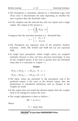
Max(0.543, 0.0, 0.459) = 0.543, so color is best. Make the root node's
attribute color and partition the examples for the resulting children
nodes as shown :
The children associated with values green and blue are uniform,
containing only – and + examples, respectively. So make these
children leaves with classifications – and +, respectively.
Q.6 Explain impurity measures in decision tree.
Ans. : · The node impurity makes reference to the mixture of
classes in the training examples covered by the node. When all the
examples in a given node belong to the same problem class, then
the node is said to be pure. The more equal proportions of classes
there are in a node, the more impure the node is.
Let |D| = Total number of data entries.
|D |
i = Number of data entries classified as i
pi =
|D |
|D|
i
= Ratio of instance classified as i.
· Impurity measure defines how well e classes are separated. In
general the impurity measure should satisfy : Largest when data
are split evenly for attribute values
®
Color
R G B
[1, 3, 5]
+, –, +
[4, 6]
–, –
[2]
+

pi =
1
Number of classes
Should be 0 when all data belong to the same class.
· Two methods are used for measuring impurity : Gini Index and
Entropy based measure
· Entropy based measure
I(D) = Entropy (D) = – p log p
i i
i 1
k
=
å
Example for k = 2
· Gini Index measure :
I(D) = Gini (D) = 1-
=
åpi
2
i 1
k
· Here, the sum is always extended to all classes. This is a very
common measure and it is used as a default value by scikit-learn.
· Given a sample, the Gini impurity measures the probability of a
misclassification if a label is randomly chosen using the
probability distribution of the branch.
®
0
0
0.1 0.2 0.3 0.4 0.5 0.6 0.7 0.8 0.9
0.1
0.2
0.3
0.4
0.5
0.6
0.7
Fig. Q.6.1

Q.7 Explain decision tree classification with Scikit-learn.
Ans. : Decision Tree Classification with Scikit-Learn
· scikit-learn contains the "DecisionTreeClassifier" class, which can
train a binary decision tree with Gini and cross-entropy impurity
measures.
· DecisionTreeClassifier accepts (as most learning methods) several
hyperparameters that control its behavior. In this case, we used
the Information Gain (IG) criterion for splitting learning data,
told the method to build a tree of at most three levels, and to
accept a node as a leaf if it includes at least five training
instances.
· let's consider a dataset with three features and three classes :
from sklearn.datasets import make_classification
· Entropy is a measure of disorder in a set, if we have zero
entropy, it means all values are the same, while it reaches its
maximum when there is an equal number of instances of each
class.
· At each node, we have a certain number of instances and we
measure its entropy.
· Let's consider a classification with default Gini impurity :
from sklearn.tree import DecisionTreeClassifier
from sklearn.model_selection import cross_val_score
· To export a trained tree, it is necessary to use the built-in
function export_graphviz():
from sklearn.tree import export_graphviz
5.2 : Ensemble Learning
Q.8 Write a note on : Ensemble Learning.
Ans. : · The idea of ensemble learning is to employ multiple
learners and combine their predictions. If we have a committee of
®

M models with uncorrelated errors, simply by averaging them the
average error of a model can be reduced by a factor of M.
· Unfortunately, the key assumption that the errors due to the
individual models are uncorrelated is unrealistic; in practice, the
errors are typically highly correlated, so the reduction in overall
error is generally small.
· Ensemble modeling is the process of running two or more related
but different analytical models and then synthesizing the results
into a single score or spread in order to improve the accuracy of
predictive analytics and data mining applications.
· Ensemble of classifiers is a set of classifiers whose individual
decisions combined in some way to classify new examples.
· Ensemble methods combine several decision trees classifiers to
produce better predictive performance than a single decision tree
classifier. The main principle behind the ensemble model is that a
group of weak learners come together to form a strong learner,
thus increasing the accuracy of the model.
· There are two approaches for combining models : voting and
stacking.
· In voting, no learning takes place at the meta level when
combining classifiers by a voting scheme. Label that is most
often assigned to a particular instance is chosen as the correct
prediction when using voting.
· Stacking is concerned with combining multiple classifiers
generated by different learning algorithms L LN
1 , ..., on a single
dataset S, which is composed by a feature vector Si = ( , )
x t
i i .
· The stacking process can be broken into two phases :
1. Generate a set of base-level classifiers C CN
1 , ..., Where
C L S
i i
= ( )
®

2. Train a meta-level classifier to combine the outputs of the
base-level classifiers
· Fig. Q.8.1 shows stacking frame.
· The training set for the meta-level classifier is generated through
a leave-one-out cross validation process.
" i = 1, …n and " k = 1, ....., N : Ck
i
= L (S – s )
k i
· The learned classifiers are then used to generate predictions for
s :y
i i
k
$ = C (x )
k
i
i
· The meta-level dataset consists of examples of the form
(( $ $ ), )
y ,..., y y
i
1
i
n
i , where the features are the predictions of the
®
1 2 3 4 n
···
···
···
h1
p1
h2
p2
h3
p3
hn
pn
Meta learner
H
P
Training set
Hypotheses
Predictions on
training observations
Training observations
Lest observation
Meta learner's
hypothesis
Final prediction
Fig. Q.8.1 Stacking frame

base-level classifiers and the class is the correct class of the
example in hand.
· Why do ensemble methods work?
· Based on one of two basic observations :
1. Variance reduction : If the training sets are completely
independent, it will always helps to average an ensemble
because this will reduce variance without affecting bias
(e.g.,bagging) and reduce sensitivity to individual data points.
2. Bias reduction : For simple models, average of models has
much greater capacity than single model Averaging models
can reduce bias substantially by increasing capacity, and
control variance by Citting one component at a time.
Q.9 What is Bagging ? Explain Bagging steps. List its advantages
and disadvantages.
Ans. : · Bagging is also called Bootstrap aggregating. Bagging and
boosting are meta-algorithms that pool decisions from multiple
classifiers. It creates ensembles by repeatedly randomly resampling
the training data.
· Bagging was the first effective method of ensemble learning and
is one of the simplest methods of arching. The meta-algorithm,
which is a special case of the model averaging, was originally
designed for classification and is usually applied to decision tree
models, but it can be used with any type of model for
classification or regression.
· Ensemble classifiers such as bagging, boosting and model
averaging are known to have improved accuracy and robustness
over a single model. Although unsupervised models, such as
clustering, do not directly generate label prediction for each
individual, they provide useful constraints for the joint prediction
of a set of related objects.
· For given a training set of size n, create m samples of size n by
drawing n examples from the original data, with replacement.
Each bootstrap sample will on average contain 63.2 % of the
®

unique training examples, the rest are replicates. It combines the
m resulting models using simple majority vote.
· In particular, on each round, the base learner is trained on what
is often called a "bootstrap replicate" of the original training set.
Suppose the training set consists of n examples. Then a
bootstrap replicate is a new training set that also consists of n
examples, and which is formed by repeatedly selecting uniformly
at random and with replacement n examples from the original
training set. This means that the same example may appear
multiple times in the bootstrap replicate, or it may appear not at
all.
· It also decreases error by decreasing the variance in the results
due to unstable learners, algorithms (like decision trees) whose
output can change dramatically when the training data is slightly
changed.
· Pseudocode :
1. Given training data (x , y ), ..., (x , y )
1 1 m m
2. For t = 1,..., T :
a. Form bootstrap replicate dataset St by selecting m random
examples from the training set with replacement.
b. Let h t be the result of training base learning algorithm on
St .
3. Output combined classifier :
H(x) majority (h (x), ..., h (x))
1 T
= .
Bagging Steps :
1. Suppose there are N observations and M features in training
data set. A sample from training data set is taken randomly
with replacement.
2. A subset of M features is selected randomly and whichever
feature gives the best split is used to split the node iteratively.
3. The tree is grown to the largest.
®

4. Above steps are repeated n times and prediction is given based
on the aggregation of predictions from n number of trees.
Advantages of Bagging :
1. Reduces over-fitting of the model.
2. Handles higher dimensionality data very well.
3. Maintains accuracy for missing data.
Disadvantages of Bagging :
1. Since final prediction is based on the mean predictions from
subset trees, it won't give precise values for the classification
and regression model.
Q.10 Explain boosting steps. List advantages and disadvantages of
boosting.
Ans. : Boosting Steps :
1. Draw a random subset of training samples d1 without
replacement from the training set D to train a weak learner C1
2. Draw second random training subset d2 without replacement
from the training set and add 50 percent of the samples that
were previously falsely classified/misclassified to train a weak
learner C1
3. Find the training samples d3
in the training set D on which C1
and C1 disagree to train a third weak learner C3
4. Combine all the weak learners via majority voting.
Advantages of Boosting :
1. Supports different loss function.
2. Works well with interactions.
Disadvantages of Boosting :
1. Prone to over-fitting.
2. Requires careful tuning of different hyper-parameters.
®

5.3 : Clustering Fundamentals
Q.11 What is cluster and distance based clustering? List the name
of clustering algorithm. Explain application of clustering.
Ans. : Clustering Fundamentals
· Clustering of data is a method by which large sets of data are
grouped into clusters of smaller sets of similar data. Clustering
can be considered the most important unsupervised learning
problem.
· A cluster is therefore a collection of objects which are "similar"
between them and are "dissimilar" to the objects belonging to
other clusters. Fig. Q.11.1 shows cluster.
· In this case we easily identify the 4 clusters into which the data
can be divided; the similarity criterion is distance : two or more
objects belong to the same cluster if they are "close" according to
a given distance (in this case geometrical distance). This is called
distance-based clustering.
· Clustering means grouping of data or dividing a large data set
into smaller data sets of some similarity.
· A clustering algorithm attempts to find natural groups of
components or data based on some similarity. Also, the clustering
algorithm finds the centroid of a group of data sets.
®
Fig. Q.11.1 Cluster

· To determine cluster membership, most algorithms evaluate the
distance between a point and the cluster centroids. The output
from a clustering algorithm is basically a statistical description of
the cluster centroids with the number of components in each
cluster.
· Cluster centroid : The centroid of a cluster is a point whose
parameter values are the mean of the parameter values of all the
points in the clusters. Each cluster has a well defined centroid.
· Distance : The distance between two points is taken as a
common metric to as see the similarity among the components of
a population. The commonly used distance measure is the
Euclidean metric which defines the distance between two points
p = (p , p , ...)
1 2 and q = (q , q , ...)
1 2 is given by :
d =
i 1
k
i i
2
(p q )
=
å -
· The goal of clustering is to determine the intrinsic grouping in a
set of unlabeled data. But how to decide what constitutes a good
clustering ? It can be shown that there is no absolute "best"
®
Raw data Clustering algorithm Clusters of data
Centroid

criterion which would be independent of the final aim of the
clustering. Consequently, it is the user which must supply this
criterion, in such a way that the result of the clustering will suit
their needs.
· Clustering analysis helps construct meaningful partitioning of a
large set of objects. Cluster analysis has been widely used in
numerous applications, including pattern recognition, data
analysis, image processing, etc.
· Clustering algorithms may be classified as listed below :
1. Exclusive clustering
2. Overlapping clustering
3. Hierarchical clustering
4. Probabilistic clustering
· A good clustering method will produce high quality clusters with
high intra-class similarity and low inter-class similarity. The
quality of a clustering result depends on both the similarity
measure used by the method and its implementation. The quality
of a clustering method is also measured by its ability to discover
some or all of the hidden patterns.
Examples of Clustering Applications
1. Marketing : Help marketers discover distinct groups in their
customer bases and then use this knowledge to develop targeted
marketing programs.
2. Land use : Identification of areas of similar land use in an earth
observation database.
3. Insurance : Identifying groups of motor insurance policy holders
with a high average claim cost.
4. Urban planning : Identifying groups of houses according to
their house type, value, and geographical location.
5. Seismology : Observed earth quake epicenters should be
clustered along continent faults.
®

Q.12 Explain K-means algorithm process.
Ans. : K-Means Algorithm Properties
1. There are always K clusters.
2. There is always at least one item in each cluster.
3. The clusters are non-hierarchical and they do not overlap.
4. Every member of a cluster is closer to its cluster than any other
cluster because closeness does not always involve the 'center' of
clusters.
The K-Means Algorithm Process
1. The dataset is partitioned into K clusters and the data points are
randomly assigned to the clusters resulting in clusters that have
roughly the same number of data points.
2. For each data point.
a. Calculate the distance from the data point to each cluster.
b. If the data point is closest to its own cluster, leave it where
it is.
c. If the data point is not closest to its own cluster, move it
into the closest cluster.
3. Repeat the above step until a complete pass through all the data
points results in no data point moving from one cluster to
another. At this point the clusters are stable and the clustering
process ends.
4. The choice of initial partition can greatly affect the final clusters
that result, in terms of inter-cluster and intracluster distances
and cohesion.
· K-means algorithm is iterative in nature. It converges, however
only a local minimum is obtained. It works only for numerical
data. This method easy to implement.
Q.13 Explain silhouettes.
Ans. : · Silhouette refers to a method of interpretation and
validation of clusters of data.
®

· Silhouettes are a general graphical aid for interpretation and
validation of cluster analysis. This technique is available through
the silhouette function. In order to calculate silhouettes, two types
of data are needed :
1. The collection of all distances between objects. These distances
are obtained from application of dist function on the
coordinates of the elements in mat with argument method.
2. The partition obtained by the application of a clustering
technique.
· For each element, a silhouette value is calculated and evaluates
the degree of confidence in the assignment of the element :
1. Well-clustered elements have a score near 1.
2. Poorly-clustered elements have a score near – 1.
· Thus, silhouettes indicate the objects that are well or poorly
clustered. Silhouette coefficient combines ideas of both cohesion
and separation, but for individual points, as well as clusters and
clustering's.
· For an individual point, I
a = Average distance of i to the points in the same cluster
b = min (average distance of i to points in another cluster)
Silhouette coefficient of i :
Silhouette coefficient
· Cohesion : Measures how closely related are objects in a cluster.
Separation : Measure how distinct or well-separated a cluster is
from other clusters.
®
s = 1 – a/b if a < b
a
b

Q.14 Explain density-based spatial clustering of applications with
noise. List its advantages and disadvantages.
Ans. : Density-Based Spatial Clustering of Applications with
Noise : The DBSCAN algorithm can identify clusters in large
spatial data sets by looking at the local density of database
elements, using only one input parameter.
· The DBSCAN can also determine what information should be
classified as noise or outliers.
· In DBSCAN, clustering happens based on two important
parameters :
1. neighbourhood (n) - cutoff distance of a point from (core point
- discussed below) for it to be considered a part of a cluster.
Commonly referred to as epsilon (abbreviated as eps).
2. minimum points (m) - minimum number of points required to
form a cluster. Commonly referred to as minPts.
· By using the density distribution of nodes in the database,
DBSCAN can categorize these nodes into separate clusters that
define the different classes. DBSCAN can find clusters of
arbitrary shape, as can be seen in the following Fig. Q.14.1.
· To find a cluster, DBSCAN starts with an arbitrary point p and
retrieves all points density-reachable from p with respect to Eps
and MinPts.
®
Fig. Q.14.1

· If p is a core point, this procedure yields a cluster with respect to
Eps and MinPts . If p is a border point, no points are
density-reachable from p and DBSCAN visits the next point of
the database.
· MinPts is a minimum number of points in the given
neighborhood N(p).
· Three category for each point are as follows :
1. Core point : if its density is high
2. Border point : density is low (but in the neighborhood of a
core point)
3. Noise point : any point that is not a core point nor a border
point
· Fig Q.14.2 shows category of points.
Algorithm :
1. Arbitrary select a point p
2. Retrieve all points density-reachable from p with repsect to Eps
and MinPts.
3. If p is a core point, a cluster is formed.
4. If p is a border point, no points are density-reachable from p
and DBSCAN visits the next point of the database.
5. Continue the process until all of the points have been processed
®
Border
Core
Outlier
MinPts - 5
Fig Q.14.2 : Category of points

· DBSCAN algorithm have done a good job classifying all the
clusters. The DBSCAN algorithm has a solution to all these
problems as it can find those complicated cluster shapes very
quickly, with only one assigned input parameter. A value for this
parameter is also suggested to the user.
Advantages
1. Clusters can have arbitrary shape and size
2. Number of clusters is determined automatically
3. Can separate clusters from surrounding noise
4. Can be supported by spatial index structures
Disadvantages
1. Input parameters may be difficult to determine
2. In some situations very sensitive to input parameter setting
Q.15 What is spectral clustering? List its advantages and
disadvantages.
Ans. : Spectral Clustering : · Spectral clustering techniques make
use of the spectrum (eigenvalues) of the similarity matrix of the
data to perform dimensionality reduction before clustering in fewer
dimensions. The similarity matrix is provided as an input and
consists of a quantitative assessment of the relative similarity of
each pair of points in the dataset
· Given data points x1
, … xN
, pairwise affinities Aij
= A(xi
, xj
)
· Build similarity graph shown in Fig. Q.15.1.
®
Fig. Q.15.1 : Similarity graph

· Clustering = find a cut through the graph
· Define a cut-type objective function
· The low-dimensional space is determined by the data. Spectral
clustering makes use of the spectrum of the graph for
· Projection and clustering equates to graph partition by different
min-cut criteria
Advantages :
1. Does not make strong assumptions on the statistics of the
clusters
2. Easy to implement.
3. Good clustering results.
4. Reasonably fast for sparse data sets of several thousand
elements.
Disadvantages :
1. May be sensitive to choice of parameters
2. Computationaly expensive for large datasets
5.4 : Evaluation Methods based on Ground
Q.16 What is Homogeneity ? Explain completeness.
Ans. : Homogeneity
· Homogeneity metric of a cluster labeling given a ground truth. A
clustering result satisfies homogeneity if all of its clusters contain
only data points which are members of a single class.
· This metric is independent of the absolute values of the labels : a
permutation of the class or cluster label values won't change the
score value in any way.
· To define the concepts of entropy H(X) and conditional entropy
H(X|Y), which measures the uncertainty of X given the
knowledge of Y.
®

· Therefore, if the class set is denoted as C and the cluster set as K,
H(C|K) is a measure of the uncertainty in determining the right
class after having clustered the dataset.
· To have a homogeneity score, it's necessary to normalize this
value considering the initial entropy of the class set H(C) :
h = 1-
H(C|K)
H(C)
· In scikit-learn, there's the built-in function homogeneity_score()
that can be used to compute this value : from sklearn.metrics
import homogeneity_score
Completeness
· A complementary requirement is that each sample belonging to a
class is assigned to the same cluster.
· A clustering result satisfies completeness if all the data points
that are members of a given class are elements of the same
cluster.
· This metric is independent of the absolute values of the labels : a
permutation of the class or cluster label values won't change the
score value in any way.
· This measure can be determined using the conditional entropy
H(K|C), which is the uncertainty in determining the right cluster
given the knowledge of the class. Like for the homogeneity score,
we need to normalize this using the entropy H(K) :
c = 1-
H(C|K)
H(K)
· We can compute this score (on the same dataset) using the
function completeness_score() :
from sklearn.metrics import completeness_score
Q.17 What is adjusted rand index ?
Ans. : Adjusted Rand Index
· The adjusted rand index measures the similarity between the
original class partitioning (Y) and the clustering.
®

· If total number of samples in the dataset is n, the rand index is
defined as :
R =
( )
a b
2
n
+
· Rand index is defined as the number of pairs of objects that are
either in the same group or in different groups in both partitions
divided by the total number of pairs of objects.
· The Rand index lies between 0 and 1.
· When two partitions agree perfectly, the Rand index achieves the
maximum value 1.
· A problem with Rand index is that the expected value of the
Rand index between two random partitions is not a constant.
· This problem is corrected by the adjusted Rand index that
assumes the generalized hyper-geometric distribution as the
model of randomness.
· The adjusted Rand index has the maximum value 1, and its
expected value is 0 in the case of random clusters.
· A larger adjusted Rand index means a higher agreement between
two partitions. The adjusted Rand index is recommended for
measuring agreement even when the partitions compared have
different numbers of clusters.
5.5 : Introduction to Meta Classifier
Q.18 Explain various multiclass classification.
Ans. : Multiclass Classification
· Each training point belongs to one of N different classes. The
goal is to construct a function which, given a new data point,
will correctly predict the class to which the new point belongs.
The multi-class classification problem refers to assigning each of
the observations into one of k classes.
®

· A common way to combine pair wise comparisons is by voting.
It constructs a rule for discriminating between every pair of
classes and then selecting the class with the most winning
two-class decisions. Though the voting procedure requires just
pair wise decisions, it only predicts a class label.
· Example of Multi-label classification is as follows :
1. Is it eatable ?
2. Is it sweet ?
3. Is it a fruit ?
4. Is it a banana ?
1. Is it a banana ?
2. Is it an apple ?
3. Is it an orange ?
4. Is it a pineapple ?
1. Is it a banana ?
2. Is it yellow ?
3. Is it sweet ?
4. Is it round ?
Nested/Hierarchical Exclusive/Multi-class General/Structured
· Fig. Q.18.1 and Q.18.2 shows binary and multiclass classification.
Multi-class classification through binary classification :
1. One vs All (OVA) :
· For each class build a classifier for that class vs the rest. Build N
different binary classifiers.
®
X
X
X
X
X2
X1
Fig Q.18.1 Binary classification
X
X
X
X
X2
X1
X
Fig Q.18.2 Multi-class classification

· For this approach, we require N = K binary classifiers, where the
kth classifier is trained with positive examples belonging to class
k and negative examples belonging to the other K – 1 classes.
· When testing an unknown example, the classifier producing the
maximum output is considered the winner, and this class label is
assigned to that example.
· It is simple and provides performance that is comparable to other
more complicated approaches when the binary classifier is tuned
well.
2. All-vs-All (AVA) :
· For each class build a classifier for those class vs the rest. Build
N (N – 1) classifiers, one classifier to distinguish each pair of
classes i and j .
· A binary classifier is built to discriminate between each pair of
classes, while discarding the rest of the classes.
· When testing a new example, a voting is performed among the
classifiers and the class with the maximum number of votes wins.
3. Calibration
· The decision function f of a classifier is said to be calibrated or
well-calibrated if P (x is correctly classified | f(x) = s) ~
- s
· Informally f is a good estimate of the probability of classifying
correctly a new datapoint x which would have output value x.
Intuitively if the "raw" output of a classifier is g you can calibrate
it by estimating the probability of x being well classified given
that g(x) = y for all y values possible.
4. Error-Correcting Output-Coding (ECOC)
· Error correcting code approaches try to combine binary classifiers
in a way that lets you exploit de-correlations and correct errors.
· This approach works by training N binary classifiers to
distinguish between the K different classes. Each class is given a
codeword of length N according to a binary matrix M . Each row
of M corresponds to a certain class.
®

· The following table shows an example for K = 5 classes and
N = 7 bit code words.
f1 f2 f3 f4 f5 f6 f7
Class 1 0 0 0 0 0 0 0
Class 2 0 1 1 0 0 1 1
Class 3 0 1 1 1 1 0 0
Class 4 1 0 1 1 0 1 0
Class 5 1 1 0 1 0 0 1
Each class is given a row of the matrix. Each column is used to
train a distinct binary classifier. When testing an unseen example,
the output codeword from the N classifiers is compared to the
given K code words, and the one with the minimum hamming
distance is considered the class label for that example.
Q.19 Explain concepts of weak and eager learner.
Ans. : Concepts of weak and eager learner
· Eager learning is a learning method in which the system tries to
construct a general, input-independent target function during
training of the system, as opposed to lazy learning, where
generalization beyond the training data is delayed until a query
is made to the system.
· Combining several weak learners to give a strong learner. It is a
kind of multiclassifier systems and meta-learners. Ensemble
typically applied to a single type of weak learner.
· Lazy learning (e.g., instance-based learning) : Simply stores
training data (or only minor processing) and waits until it is
given a test tuple
· Eager learning (the above discussed methods) : Given a set of
training tuples, constructs a classification model before receiving
new (e.g., test) data to classify
· Lazy : less time in training but more time in predicting
®

· Lazy method effectively uses a richer hypothesis space since it
uses many local linear functions to form an implicit global
approximation to the target function
· Eager : must commit to a single hypothesis that covers the entire
instance space
END…?
®

6.1 : Hierarchical Clustering
Q.1 What is hierarchical clustering ? Explain in detail.
Ans. : · Hierarchical clustering is a widely used data analysis tool.
The idea is to build a binary tree of the data that successively
merges similar groups of points. Visualizing this tree provides a
useful summary of the data.
· Hierarchical clustering is based on the general concept of finding
a hierarchy of partial clusters, built using either a bottom-up or a
top-down approach.
· Hierarchical clustering can be performed with either a distance
matrix or raw data. When raw data is provided, the software will
automatically compute a distance matrix in the background.
· This method use distance matrix as clustering criteria. This
method does not require the number of clusters K as an input,
but needs a termination condition.
· Hierarchical clustering is a widely used data analysis tool.
· The idea is to build a binary tree of the data that successively
merges similar groups of points. Visualizing this tree provides a
useful summary of the data.
· Hierarchical clustering arranges items in a hierarchy with a
treelike structure based on the distance or similarity between
them.
· The graphical representation of the resulting hierarchy is a
tree-structured graph called a dendrogram.
®
6 Clustering Techniques
UNIT - VI
(6 - 1)

· The main output of Hierarchical Clustering is a dendrogram,
which shows the hierarchical relationship between the clusters
· Hierarchical clustering methods can be further classified as either
agglomerative or divisive, depending on whether the hierarchical
decomposition is formed in a bottom-up (merging) or top-down
(splitting) fashion.
· Hierarchical clustering does not require the specification of a
pre-defined number of clusters. Fig. Q.1.1 shows clustering and
hierarchical clustering.
Machine Learning 6 - 2 Clustering Techniques
®
Fig. Q.1.1 (a) Clustering
E1 E2
E3
E4 E7 E8
E
E2
E
E1
E7
E8
Fig. Q.1.1 (b) Hierarchical clustering

· Use distance matrix as clustering criteria. This method does not
require the number of clusters k as an input, but needs a
termination condition
· The core idea of hierarchical clustering is to create different levels
of clusters. Each upper level cluster is conceptually the result of a
merging of the clusters at lower levels. At the lowest level each
cluster contains a single observation. At the highest level there is
a single cluster that contains all observations.
Q.2 Explain agglomerative hierarchical clustering.
Ans. : · This bottom-up strategy starts by placing each object in its
own cluster and then merges these atomic clusters into larger and
larger clusters, until all of the objects are in a single cluster or until
certain termination conditions are satisfied.
· Hierarchical clustering typically works by sequentially merging
similar clusters, as shown above. This is known as agglomerative
hierarchical clustering.
· Initially, AGNES places each objects into a cluster of its own. The
clusters are then merged step-by-step according to some criterion.
· For example, cluster C1 and C2 may be merged if an object in C1
and object in C2 form the minimum Euclidean distance between
any two objects from different clusters.
· In the agglomerative hierarchical approach, we start by defining
each data point to be a cluster and combine existing clusters at
each step.
Steps :
1. Compute the Euclidean Distance between every pair of
patterns. Let the smallest distance be between patterns Xi and
Xj.
2. Create a cluster C composed of Xi and Xj. Replace Xi and Xj
by cluster vector C in the training set (the average of Xi and
Xj).
®

3. Go back to 1, treating clusters as points, though with an
appropriate weight, until no point is left.
· Fig. Q.2.1 shows working of both cluster.
· Each level of the hierarchy represents a specific grouping of the
whole data set into disjoint clusters.
· The user must provide an additional criterion in order to extract
from a hierarchical clustering an ordinary clustering: a criterion
to pick the level of the hierarchy that corresponds to the natural
clustering. One such criterion is the gap statistic.
· Since hierarchical clustering is a greedy search algorithm based
on a local search, the merging decision made early in the
agglomerative process are not necessarily the right ones.
Q.3 What is dendrogram ? Explain with example.
Ans. : · Decompose data objects into a several levels of nested
partitioning (tree of clusters), called a dendrogram. A clustering of
the data objects is obtained by cutting the dendrogram at the
desired level, then each connected component forms a cluster.
· The agglomerative hierarchical clustering algorithms available in
this program module build a cluster hierarchy that is commonly
displayed as a tree diagram called a dendrogram.
· They begin with each object in a separate cluster. At each step,
the two clusters that are most similar are joined into a single new
®
Step 0 Step 1 Step 2 Step 3 Step 4
divisive
(DIANA)
agglomerative
(AGNES)
Step 0
Step 1
Step 2
Step 3
Step 4
a
b
c
d
e
a b
d e
c d e
a b c d e
Fig. Q.2.1

cluster. Once fused, objects are never separated. The eight
methods that are available represent eight methods of defining
the similarity between clusters.
· Suppose we wish to cluster the bivariate data shown in the
following scatter plot. In this case, the clustering may be done
visually. The data have three clusters and two singletons, 6 and
13.
· Following is a dendrogram of the results of running these data
through the Group Average clustering algorithm.
· The horizontal axis of the dendrogram represents the distance or
dissimilarity between clusters. The vertical axis represents the
objects and clusters. The dendrogram is fairly simple to interpret.
Remember that our main interest is in similarity and clustering.
· Each joining of two clusters is represented on the graph by the
splitting of a horizontal line into two horizontal lines. The
horizontal position of the split, shown by the short vertical bar,
gives the distance (dissimilarity) between the two clusters.
· Looking at this dendrogram, you can see the three clusters as
three branches that occur at about the same horizontal distance.
®
Fig. Q.3.1

The two outliers, 6 and 13, are fused in rather arbitrarily at much
higher distances. This is the interpretation.
Q.4 Explain connectivity constraints of clustering.
Ans. : · Scikit-learn also allows specifying a connectivity matrix,
which can be used as a constraint when finding the clusters to
merge.
®
Fig. Q.3.2 Dendrogram

· In this way, clusters which are far from each other (nonadjacent
in the connectivity matrix) are skipped.
· A very common method for creating such a matrix involves
using the k-nearest neighbors graph function, that is based on
the number of neighbors a sample has.
sklearn.datasets.make_circles(n_samples = 100,
shuffle=True,noise=None, random_state=None, factor=0.8)
· It makes a large circle containing a smaller circle in 2d. A simple
toy dataset to visualize clustering and classification algorithms.
Parameters :
1. n_samples : int, optional (default=100) ® The total number of
points generated. If odd, the inner circle will have one point
more than the outer circle.
2. shuffle : bool, optional (default=True) ® Whether to shuffle the
samples.
3. noise : double or None (default=None) ® Standard deviation of
Gaussian noise added to the data.
4. random_state : int, RandomState instance or None (default) ®
Determines random number generation for dataset shuffling
and noise. Pass an int for reproducible output across multiple
function calls. See Glossary.
5. factor : 0 < double < 1 (default=.8) ® Scale factor between
inner and outer circle.
6.2 : Introduction to Recommendation Systems
Q.5 What is a recommendation systems ?
Ans. : · Recommendation system is a subclass of information
filtering system that seeks to predict the "rating" or "preference" a
user would give to an item.
· Recommender Systems (RSs) are software tools and techniques
providing suggestions for items to be of use to a user.
®

· The suggestions relate to various decision-making processes, such
as what items to buy, what music to listen to, or what online
news to read. Item is the general term used to denote what the
system recommends to users.
· Recommender systems typically produce a list of
recommendations in one of two ways, through collaborative
filtering or through content-based filtering.
· Collaborative filtering systems work by collecting user remark in
the form of ratings for items in a given field and exploiting
similarities in rating actions amongst several users in determining
how to recommend an item. Collaborative filtering systems
recommend an item to a user based on opinions of other users.
· Content-Based Recommending : Recommendations are based on
information on the content of items rather than on other users'
opinions. Uses a machine learning algorithm to induce a profile
of the users preferences from examples based on a feature
description of content.
Q.6 Explain the following :
a) Naïve user based systems b) Content based systems
Ans. : a) Naïve user based systems :
· Na&&
ive Bayes is a probabilistic approach to inductive learning, and
belongs to the general class of Bayesian classifiers. These
approaches generate a probabilistic model based on previously
observed data.
· Let us assume, a set of users represented by feature vectors.
U = {u , u ,....., u }
1 2 n where u R
n
n
Î
· The set of items are represented by
I = {i , i , ....., i }
1 2 m
· Let's assume also that there is a relation which associates each
user with a subset of items, items for which an explicit action or
feedback has been performed:
g(u) {i , i , ....., i }
1 2 k
® where k (0, m)
Î
®

· In a user-based system, the users are periodically clustered and
therefore, considering a generic user u, we can immediately
determine the ball containing all the users who are similar to our
sample :
B (u)
R = {u , u ,....., u }
1 2 k
b) Content based systems :
· Any systems implementing a content-based recommendation
approach analyze a set of documents and/or descriptions of items
previously rated by a user, and build a model or profile of user
interests based on the features of the objects rated by that user.
· The recommendation process basically consists in matching up
the attributes of the user profile against the attributes of a content
object.
· The result is a relevance judgment that represents the user"s level
of interest in that object. If a profile correctly reflects user
preferences, it is of tremendous advantage for the effectiveness of
an information access process.
· Advantages of Content-Based Approach :
1. No need for data on other users.
2. Able to recommend to users with unique tastes.
3. Able to recommend new and unpopular items
4. Can provide explanations of recommended items by listing
content-features that caused an item to be recommended.
· Disadvantages of Content-Based Method
1. Requires content that can be encoded as meaningful features.
2. Users' tastes must be represented as a learnable function of
these content features.
3. Unable to exploit quality judgments of other users.
®

6.3 : Model Free Collaborative Filtering
Q.7 What is collaborative filtering ? Explain model free
collaborative filtering.
Ans. : · Collaborative filtering is a method of making automatic
predictions (filtering) about the interests of a single user by
collecting preferences or taste information from many users
(collaborating).
· Collaborative Filtering (CF) uses given rating data by many users
for many items as the basis for predicting missing ratings and/or
for creating a top-N recommendation list for a given user, called
the active user.
· Formally, we have a set of users U = {u1
, u2
, . . . , um
} and a set
of items I = {i1
, i2
, . . . , in
}. Ratings are stored in "m ´ n"
user-item rating matrix.
· The problem of collaborative filtering is to predict how well a
user will like an item that he has not rated given a set of
historical preference judgments for a community of users.
· Here we try to model a user-item matrix based on the
preferences of each user (rows) for each item (columns). For
example :
Mu I
´ =
0 1 4 3 0 4 3 5
2 1 2 3 0 0 4 1
0 2 0 3 1 2 4 2
5 0 0 1 2 1 3 1
3 0 0 3 0 1 0 4
1 4 1 0 3
L
L
L
L
L
5 0 3
0 2 3 1 2 4 4 0
1 3 2 0 0 2 2 1
L
M M M M M M M M M
L
L
æ
è
ç
ç
ç
ç
ç
ç
ç
ç
ç
ç
ç
ç
ö
ø
÷
÷
÷
÷
÷
÷
÷
÷
÷
÷
÷
÷
· The ratings are bounded between 1 and 5 (0 means no rating)
and our goal is to cluster the users according to their rating
vector.
®

· In order to build the model, we first need to define the user-item
matrix as a Python dictionary with the structure:
{user_1 : { item1: rating, item2: rating, ... }, ..., user_n: ...}
Q.8 Explain user based and item based collaborative filtering.
Ans. : · There are two types of collaborative filtering algorithms:
user based and item based.
1. User based
· User-based collaborative filtering algorithms work off the premise
that if a user (A) has a similar profile to another user (B), then A
is more likely to prefer things that B prefers when compared
with a user chosen at random.
· The assumption is that users with similar preferences will rate
items similarly. Thus missing ratings for a user can be predicted
by first finding a neighborhood of similar users and then
aggregate the ratings of these users to form a prediction.
· The neighborhood is defined in terms of similarity between users,
either by taking a given number of most similar users (k nearest
neighbors) or all users within a given similarity threshold.
· Popular similarity measures for CF are the Pearson correlation
coefficient and the Cosine similarity.
· For example, a collaborative filtering recommendation system for
television tastes could make predictions about which television
show a user should like given a partial list of that user's tastes
(likes or dislikes).
· Note that these predictions are specific to the user, but use
information gleaned from many users. This differs from the
simpler approach of giving an average score for each item of
interest, for example based on its number of votes.
· User-based CF is a memory-based algorithm which tries to
mimics word-of mouth by analyzing rating data from many
individuals.
®

· The two main problems of user-based CF are that the whole user
database has to be kept in memory and that expensive similarity
computation between the active user and all other users in the
database has to be performed.
2. Item-based collaborative filtering
· Item-based CF is a model-based approach which produces
recommendations based on the relationship between items
inferred from the rating matrix.
· The assumption behind this approach is that users will prefer
items that are similar to other items they like.
· The model-building step consists of calculating a similarity matrix
containing all item-to-item similarities using a given similarity
measure.
· Popular are again Pearson correlation and Cosine similarity. All
pair-wise similarities are stored in n × n similarity matrix S.
· Item-based collaborative filtering has become popularized due to
its use by YouTube and Amazon to provide recommendations to
users.
· This algorithm works by building an item-to-item matrix which
defines the relationship between pairs of items.
· When a user indicates a preference for a certain type of item, the
matrix is used to identify other items with similar characteristics
that can also be recommended.
· Item-based CF is more efficient than user-based CF since the
model is relatively small (N × k) and can be fully pre-computed.
Item-based CF is known to only produce slightly inferior results
compared to user-based CF and higher order models which take
the joint distribution of sets of items into account are possible.
®

Q.9 Discuss memory based and model based algorithm ? List its
advantages and disadvantages.
Ans. : 1. Memory-based algorithms :
· Operate over the entire user-item database to make predictions.
· Statistical techniques are employed to find the neighbors of the
active user and then combine their preferences to produce a
prediction.
· Memory-based algorithms utilize the entire user-item database to
generate a prediction. These systems employ statistical techniques
to find a set of users, known as neighbors that have a history of
agreeing with the target user.
· Once a neighborhood of users is formed, these systems use
different algorithms to combine the preferences of neighbors to
produce a prediction or top-N recommendation for the active
user. The techniques, also known as nearest-neighbor or
user-based collaborative filtering are more popular and widely
used in practice.
· Dynamic structure. More popular and widely used in practice.
Advantages
1. The quality of predictions is rather good.
2. This is a relatively simple algorithm to implement for any
situation.
3. It is very easy to update the database, since it uses the entire
database every time it makes a prediction.
Disadvantages
1. It uses the entire database every time it makes a prediction, so it
needs to be in memory it is very, very slow.
2. Even when in memory, it uses the entire database every time it
makes a prediction, so it is very slow.
3. It can sometimes not make a prediction for certain active
users/items. This can occur if the active user has no items in
common with all people who have rated the target item.
®

4. Overfits the data. It takes all random variability in people's
ratings as causation, which can be a real problem. In other
words, memory-based algorithms do not generalize the data at
all.
2. Model-based algorithms :
· Input the user database to estimate or learn a model of user
ratings, then run new data through the model to get a predicted
output.
· A prediction is computed through the expected value of a user
rating, given his/her ratings on other items.
· Static structure. In dynamic domains the model could soon
become inaccurate.
· Model-based collaborative filtering algorithms provide item
recommendation by first developing a model of user ratings.
Algorithms in this category take a probabilistic approach and
envision the collaborative filtering process as computing the
expected value of a user prediction, given his/her ratings on other
items.
· The model building process is performed by different machine
learning algorithms such as Bayesian network, clustering and
rule-based approaches. The Bayesian network model formulates a
probabilistic model for collaborative filtering problem.
· The clustering model treats collaborative filtering as a
classification problem and works by clustering similar users in
same class and estimating the probability that a particular user is
in a particular class C and from there computes the conditional
probability of ratings.
· The rule-based approach applies association rule discovery
algorithms to find association between co-purchased items and
then generates item recommendation based on the strength of the
association between items.
®

Advantages
1. Scalability : Most models resulting from model-based algorithms
are much smaller than the actual dataset, so that even for very
large datasets, the model ends up being small enough to be
used efficiently. This imparts scalability to the overall system.
2. Prediction speed : Model-based systems are also likely to be
faster, at least in comparison to memory-based systems because,
the time required to query the model is usually much smaller
than that required to query the whole dataset.
3. Avoidance of over fitting : If the dataset over which we build
our model is representative enough of real-world data, it is
easier to try to avoid over-fitting with model-based systems.
Disadvantages
1. Inflexibility : Because building a model is often a time- and
resource-consuming process, it is usually more difficult to add
data to model-based systems, making them inflexible.
2. Quality of predictions : The fact that we are not using all the
information (the whole dataset) available to us, it is possible
that with model-based systems, we don't get predictions as
accurate as with model-based systems. It should be noted,
however, that the quality of predictions depends on the way the
model is built. In fact, as can be seen from the results page, a
model-based system performed the best among all the
algorithms we tried.
Q.10 Briefly discuss singular value decomposition.
Ans. : · Singular Value Decomposition (SVD) is a matrix
factorization technique commonly used for producing low-rank
approximations.
· The singular value decomposition of a matrix A is the
factorization of A into the product of three matrices A = UDVT
where the columns of U and V are ortho-normal and the matrix
D is diagonal with positive real entries.
®

· The columns of V in the singular value decomposition, called the
right singular vectors of A, always form an orthogonal set with
no assumptions on A. The columns of U are called the left
singular vectors and they also form an orthogonal set.
· The singular values are the diagonal entries of the S matrix and
are arranged in descending order. The singular values are always
real numbers. If the matrix A is a real matrix, then U and V are
also real.
· To understand how to solve for SVD, let's take the example of
the matrix :
A =
2 4
1 3
0 0
0 0
é
ë
ê
ê
ê
ê
ù
û
ú
ú
ú
ú
· In this example the matrix is a 4 ´ 2 matrix. We know that for an
n ´ n matrix W, then a nonzero vector x is the eigenvector of W
if : W x = l x
· For some scalar l. Then the scalar l is called an eigenvalue of A,
and x is said to be an eigenvector of A corresponding to l .
· So to find the eigenvalues of the above entity we compute
matrices AAT and A A
T As previously stated, the eigenvectors
of AAT make up the columns of U so we can do the following
analysis to find U.
AAT =
2 4
1 3
0 0
0 0
2 4 0 0
1 3 0 0
é
ë
ê
ê
ê
ê
ù
û
ú
ú
ú
ú
é
ë
ê
ù
û
ú =
20 14 0 0
14 10 0 0
0 0 0 0
0 0 0 0
é
ë
ê
ê
ê
ê
ù
û
ú
ú
ú
ú
= W
· "Now that we have a n x n matrix we can determine the
eigenvalues of the matrix W.
Since W x = l x then (W - lI) x = 0
®

20 14 0 0
14 10 0 0
0 0 0
0 0 0
-
-
-
-
é
ë
ê
ê
ê
ê
ù
û
ú
ú
ú
ú
l
l
l
l
.x = (W – lI) x = 0
· For a unique set of eigenvalues to determinant of the matrix
( )
W I
- l must be equal to zero. Thus from the solution of the
characteristic equation, |W - lI|= 0.
· SVD-based recommendation generation technique leads to very
fast online performance, requiring just a few simple arithmetic
operations for each recommendation but computing the SVD is
very expensive.
6.4 Fundamentals of Deep Networks
Q.11 Explain deep learning. What are the challenges in deep
learning ?
Ans. : · Deep Learning is a new area of machine learning research,
which has been introduced with the objective of moving machine
learning closer to one of its original goals.
· Deep learning is about learning multiple levels of representation
and abstraction that help to make sense of data such as images,
sound, and text.
· 'Deep learning' means using a neural network with several layers
of nodes between input and output. It is generally better than
other methods on image, speech and certain other types of data
because the series of layers between input and output do feature
identification and processing in a series of stages, just as our
brains seem to.
· Deep learning emphasizes the network architecture of today's
most successful machine learning approaches. These methods are
based on "deep" multi-layer neural networks with many hidden
layers.
Challenges in Deep learning :
· They need to find and process massive datasets for training.
®

· One of the reasons deep learning works so well is the large
number of interconnected neurons, or free parameters, that allow
for capturing subtle nuances and variations in data.
· Due to the sheer number of layers, nodes, and connections, it is
difficult to understand how deep learning networks arrive at
insights.
· Deep-learning networks are highly susceptible to the butterfly
effect-small variations in the input data can lead to drastically
different results, making them inherently unstable.
Q.12 What is neuron ? Explain basic components of biological
neurons.
Ans. : · Artificial neural systems are inspired by biological neural
systems. The elementary building block of biological neural systems
is the neuron.
· The brain is a collection of about 10 billion interconnected
neurons. Each neuron is a cell [right] that uses biochemical
reactions to receive, process and transmit information. Fig. Q.12.1
shows biological neural systems.
· The single cell neuron consists of the cell body or soma, the
dendrites and the axon. The dendrites receive signals from the
axons of other neurons. The small space between the axon of one
neuron and the dendrite of another is the synapse. The afferent
dendrites conduct impulses toward the soma. The efferent axon
conducts impulses away from the soma.
®
Dendrite Nucleus
Soma Axon
Axon hillock
Terminal buttons
Fig. Q.12.1 Schematic of biological neuron

Basic Components of Biological Neurons
1. The majority of neurons encode their activations or outputs as a
series of brief electrical pulses (i.e. spikes or action potentials).
2. The neuron's cell body (soma) processes the incoming
activations and converts them into output activations.
3. The neuron's nucleus contains the genetic material in the form
of DNA. This exists in most types of cells, not just neurons.
4. Dendrites are fibres which emanate from the cell body and
provide the receptive zones that receive activation from other
neurons.
5. Axons are fibres acting as transmission lines that send activation
to other neurons.
6. The junctions that allow signal transmission between the axons
and dendrites are called synapses. The process of transmission is
by diffusion of chemicals called neurotransmitters across the
synaptic cleft.
· Comparison between Biological NN and Artificial NN
Biological NN Artificial NN
soma unit
Axon, dendrite Dendrite
Synapse Weight
Potential Weighted sum
Threshold Bias weight
Signal Activation
Q.13 Define activation function. What is necessity of activation
functions ?
Ans. : · Activation function decides, whether a neuron should be
activated or not by calculating weighted sum and further adding
bias with it. The purpose of the activation function is to introduce
non-linearity into the output of a neuron.
®

· In a neural network, each neuron has an activation function
which specifies the output of a neuron to a given input. Neurons
are switches that output 1 when they are sufficiently activated
and a 0 when not.
Q.14 Define activation function. Explain the purpose of activation
function in multilayer neural networks. Give any two activation
functions.
Ans. : · An activation function f performs a mathematical
operation on the signal output. The activation functions are chosen
depending upon the type of problem to be solved by the network.
There are a number of common activation functions in use with
neural networks.
· Fig. Q.14.1 shows position of activation function. Unit step
function is one of the activation function.
· The cell body itself is considered to have two functions. The first
function is integration of all weighted stimuli symbolized by the
summation sign. The second function is the activation which
transforms the sum of weighted stimuli to an output value which
is sent out through connection y.
· Typically the same activation function is used for all neurons in
any particular layer. In a multi-layer network if the neurons have
linear activation functions the capabilities are no better than a
®
( )
Threshold
j
x1
x2
x3
xn
Inputs Weights
W1j
W3j
Wnj
W2j
f
Transfer
function
Activation
function
Net input
(net )
j
o
Activation
j
Fig. Q.14.1 Position of activation function

single layer network with a linear activation function. Hence in
most cases nonlinear activation functions are used.
1. Linear activation function : The linear activation function will
only produce positive numbers over the entire real number
range. The linear activation function value is 0 if the argument
is less than a lower boundary, increasing linearly from 0 to +1
for arguments equal or larger than the lower boundary and less
than an upper boundary, and +1 for all arguments equal or
greater than a given upper boundary.
2. Sigmoid activation function : The sigmoid function will only
produce positive numbers between 0 and 1. The sigmoid
activation function is most used for training data that is also
between 0 and 1. It is one of the most used activation functions.
A sigmoid function produces a curve with an "S" shape. Logistic
and hyperbolic tangent functions are commonly used sigmoid
functions. The sigmoid functions are extensively used in back
propagation neural networks because it reduces the burden of
complication involved during training phase.
sig(t) =
1
1+ -
e t
®
+1
–1
1
0.9
0.8
0.7
0.6
0.5
0.4
0.3
0.2
0.1
0
0
– 2
– 4
– 6 2 4 6
Fig. Q.14.2 (a) Linear functions Fig. Q.14.2 (b) Sigmoid functions

3. Binary sigmoid : The logistic function, which is a sigmoid
function between 0 and 1 are used in neural network as
activation function where the output values are either binary or
varies from 0 to 1. It is also called as binary sigmoid or logistic
sigmoid.
f (x) =
1
1+ -
e x
4. Bipolar sigmoid : A logistic sigmoid function can be scaled to
have any range of values which may be appropriate for a
problem. The most common range is from –1 to 1. This id called
bipolar sigmoid.
f (x) = –1 +
2
1+ -
e x
The bipolar sigmoid is also closely related to the hyperbolic tangent
function.
tan h (x) =
exp (x) exp ( x)
exp (x) exp ( x)
- -
+ -
=
1 exp ( 2x)
1 exp ( 2x)
- -
+ -
Q.15 What is perceptron ? Define the architecture of a perceptron ?
Ans. : · The perceptron is a feed - forward network with one
output neuron that learns a separating hyper - plane in a pattern
space.
®
1
f(x)
Fig. Q.14.2 (c) Binary sigmoid function

· The "n" linear Fx neurons feed forward to one threshold output
Fy neuron. The perceptron separates linearly set of patterns.
Architecture of a perceptron :
· The perceptron is a feed-forward network with one output
neuron that learns a separating hyper-plane in a pattern space.
The "n" linear Fx neurons feed forward to one threshold output
patterns.
· SLP is the simplest type of artificial neural networks and can
only classify linearly separable cases with a binary target (1 , 0).
· We can connect any number of McCulloch-Pitts neurons together
in any way we like. An arrangement of one input layer of
McCulloch-Pitts neurons feeding forward to one output layer of
McCulloch-Pitts neurons is known as a Perceptron.
· A single layer feed-forward network consists of one or more
output neurons, each of which is connected with a weighting
factor Wij to all of the inputs Xi .
· The Perceptron is a kind of a single-layer artificial network with
only one neuron. The Percepton is a network in which the
neuron unit calculates the linear combination of its real-valued or
boolean inputs and passes it through a threshold activation
function. Fig. Q.15.1 shows Perceptron.
®
Weight
W1
Weight
W2
Weight
WN
S
Input 1
Input 2
Input N
·
·
·
Threshold
Output
Sigmoid
Fig. Q.15.1

· The Perceptron is sometimes referred to a Threshold Logic Unit
(TLU) since it discriminates the data depending on whether the
sum is greater than the threshold value.
· In the simplest case the network has only two inputs and a single
output. The output of the neuron is :
y = f W X b
i 1
2
i i
=
å +
æ
è
ç
ç
ö
ø
÷
÷
· Suppose that the activation function is a threshold then
f =
1 if s 0
1 if s 0
>
- £
ì
í
î
· The Perceptron can represent most of the primitive boolean
functions : AND, OR, NAND and NOR but can not represent
XOR.
· In single layer perceptron, initial weight values are assigned
randomly because it does not have previous knowledge. It sum
all the weighted inputs. If the sum is greater than the threshold
value then it is activated i.e. output = 1.
Output
W X W X ... W X
1 1 2 2 n n
+ + + > q Þ 1
W X W X ... W X
1 1 2 2 n n
+ + + £ q Þ 0
· The input values are presented to the perceptron, and if the
predicted output is the same as the desired output, then the
performance is considered satisfactory and no changes to the
weights are made.
· If the output does not match the desired output, then the weights
need to be changed to reduce the error.
· The weight adjustment is done as follows :
DW = h d x
´ ´
Where
X = Input data
®

d = Predicted output and desired output.
h = Learning rate
· If the output of the perceptron is correct then we do not take any
action. If the output is incorrect then the weight vector is
W W W
® + D .
· The process of weight adaptation is called learning.
· Perceptron Learning Algorithm :
1. Select random sample from training set as input.
2. If classification is correct, do nothing.
3. If classification is incorrect, modify the weight vector W using
Wi = W d (n) X (n)
i i
+h
Repeat this procedure until the entire training set is classified
correctly.
Q.16 What do you mean by zero-centering ?
Ans. : · Feature normalization is often required to neutralize the
effect of different quantitative features being measured on different
scales. If the features are approximately normally distributed, we
can convert them into z-scores by centring on the mean and
dividing by the standard deviation. If we don't want to assume
normality we can centre on the median and divide by the
interquartile range.
· Sometimes feature normalization is understood in the stricter
sense of expressing the feature on a [0,1] scale. If we know the
feature's highest and lowest values h and l, then we can simply
apply the linear scaling.
· Feature calibration is understood as a supervised feature
transformation adding a meaningful scale carrying class
information to arbitrary features. This has a number of important
advantages. For instance, it allows models that require scale, such
as linear classifiers, to handle categorical and ordinal features. It
®

also allows the learning algorithm to choose whether to treat a
feature as categorical, ordinal or quantitative.
· The goal of both types of normalization is to make it easier for
your learning algorithm to learn. In feature normalization, there
are two standard things to do :
1. Centering : Moving the entire data set so that it is centered
around the origin.
2. Scaling : Rescaling each feature so that one of the following
holds :
a) Each feature has variance 1 across the training data.
b) Each feature has maximum absolute value 1 across the
training data.
· The goal of centering is to make sure that no features are
arbitrarily large.
Q.17 Write short note on Tanh and ReLU neurons.
Ans. : · Tanh is also like logistic sigmoid but better. The range of
the tanh function is from (-1 to 1). Tanh is also sigmoidal
(s - shaped).
· Fig. Q.17.1 shows tanh v/s Logistic Sigmoid.
®
Sigmoid
Tanh
1
0.5
f(x)
0
–0.5
–1
–3 –2 –1 0 1 2 3
X
Fig. Q.17.1 : tanh v/s Logistic Sigmoid

· Tanh neuron is simply a scaled sigmoid neuron.
· Problems resolved by Tanh
1. The output is not zero centered
2. Small gradient of sigmoid function
· ReLU (Rectified Linear Unit) is the most used activation function
in the world right now. Since, it is used in almost all the
convolution neural networks or deep learning.
· Fig. Q.17.2 shows ReLU v/s Logistic Sigmoid.
· As you can see, the ReLU is half rectified (from bottom). f(z) is
zero when z is less than zero and f(z) is equal to z when z is
above or equal to zero.
· Compared to tanh/sigmoid neurons that involve expensive
operations (exponentials, etc.), the ReLUcan be implemented by
simply thresholding a matrix of activations at zero.
®
1.0
0.8
0.4
0.2
0.0
–5 0 5 10
0.6
(z) =
1
———
1 + e
–z
–10
Sigmoid
10
8
4
2
0
–5 0 5 10
6
–10
ReLU
R(z) = max(0, z)
Fig. Q.17.2 : ReLU v/s Logistic Sigmoid

Function Advantages Disadvantages
Sigmoid 1. Outputin range (0,1) 1. Saturated Neurons
2. Not zero entered
3. Small gradient
4. Vanishing gradient
Tanh 1. Zero centered, 1. Saturated Neurons
2. Output in range(-1,1)
ReLU 1. Computational efficiency, 1. Dead Neurons,
2. Accelerated convergence 2. Not zero centered
END...?
®

Course 2015
Time : 1 Hour] [Maximum Marks : 30
Instructions to the candidates :
1) Attempt questions Q.1 or Q.2, Q.3 or Q.4, Q.5 or Q.6.
2) Neat diagrams must be drawn wherever necessary.
3) Assume suitable data if necessary.
Q.1 a) Define machine learning and state two examples or applications
of machine learning in our day to day lives. [5]
Ans. : Refer Q.2 of Chapter - 1.
Example of machine learning :
1. Medical diagnosis : Machine learning can be used in the
techniques and tools that can help in the diagnosis of diseases. It
is used for the analysis of the clinical parameters and their
combination for the prognosis example prediction of disease
progression for the extraction of medical knowledge for the
outcome research, for therapy planning and patient monitoring.
These are the successful implementations of the machine
learning methods. It can help in the integration of
computer-based systems in the healthcare sector.
2. Image recognition is one of the most common uses of machine
learning. There are many situations where you can classify the
object as a digital image. For example, in the case of a black and
white image, the intensity of each pixel is served as one of the
measurements. In colored images, each pixel provides 3
measurements of intensities in three different colors - red, green
and blue (RGB).
b) What do you mean by supervised and unsupervised learning ?
Explain one example of each. (Refer Q.5 and Q.6 of Chapter - 1) [5]
®
APRIL-2019 [IN SEM] 245 Solved Paper
(S - 1)

OR
Q.2 a) What is Principal Component Analysis (PCA), when it is
used ? (Refer Q.15 of Chapter - 1) [5]
b) What do you mean by dictionary learning ? What are its
applications ? (Refer Q.10 of Chapter - 2) [5]
Q.3 a) Justify the statement : Raw data has a significant impact on
feature engineering process. [5]
Ans. : · Feature engineering is the process of using domain
knowledge of the data to create features that make machine
learning algorithms work.
· If feature engineering is done correctly, it increases the predictive
power of machine learning algorithms by creating features from
raw data that help facilitate the machine learning process. Feature
Engineering is an art.
· Feature engineering is the process by which knowledge of data is
used to construct explanatory variables, features, that can be used
to train a predictive model.
· Engineering and selecting the correct features for a model will not
only significantly improve its predictive power, but will also offer
the flexibility to use less complex models that are faster to run
and more easily understood
· One form of feature engineering is to decompose raw attributes
into features that will be easier to interpret patterns from.
· For example, decomposing dates or timestamp variables into a
variety of constituent parts may allow models to discover and
exploit relationships.
· Common time frames for which trends occur include : Absolute
time, day of the year, day of the week, month, hour of the day,
minute of the hour, year, etc. Breaking dates up into new features
such as this will help a model better represent structures or
seasonality in the data.
· For example, if you were investigating ice cream sales, and
created a "Season of Sale" feature, the model would recognize a
peak in the summer season.
Machine Learning S - 2 Solved University Question Papers
®

· However, an "Hour of Sale" feature would reveal an entirely
different trend, possibly peaking in the middle of each day.
b) Explain different mechanisms for managing missing features in
a dataset. (Refer Q.4 of Chapter - 2) [5]
OR
Q.4 a) With reference to feature engineering, explain data scaling and
normalization tasks. [5]
Ans. : Data scaling and normalization tasks :
· Generic dataset is made up of different values which can be
drawn from different distributions, having different scales.
Machine learning algorithm is not naturally able to distinguish
among these various situations. For this reason it is always
preferable to standardize datasets before processing them.
· Standardization : To transform data so that it has zero mean and
unit variance. Also called scaling.
· Use function sklearn.preprocessing.scale()
· Parameters :
X : Data to be scaled
with_mean : Boolean. Whether to center the data (make zero
mean)
with_std : Boolean (whether to make unit standard deviation
· Normalization : To transform data so that it is scaled to the [0,1]
range.
· Use function sklearn.preprocessing.normalize()
· Parameters :
X : Data to be normalized
norm : which norm to use : l1 or l2
axis : whether to normalize by row or column
· Normalizing in scikit-learn refers to rescaling each observation
(row) to have a length of 1.
®

· This preprocessing can be useful for sparse datasets (lots of zeros)
with attributes of varying scales when using algorithms that
weight input values such as neural networks and algorithms that
use distance measures such as K-Nearest Neighbors.
· You can normalize data in Python with scikit-learn using the
Normalizer class.
· Centering and scaling happen independently on each feature by
computing the relevant statistics on the samples in the training
set. Mean and standard deviation are then stored to be used on
later data using the transform method.
· Standardization of a dataset is a common requirement for many
machine learning estimators : they might behave badly if the
individual features do not more or less look like standard
normally distributed data.
· Examples :
>>>Hide the prompts and output>>> from sklearn.preprocessing
import StandardScaler
>>> data = [[0, 0], [0, 0], [1, 1], [1, 1]]
>>> scaler = StandardScaler()
>>> print(scaler.fit(data))
StandardScaler(copy=True, with_mean=True, with_std=True)
>>> print(scaler.mean_)
[0.5 0.5]
>>> print(scaler.transform(data))
[ [-1. -1.]
[-1. -1.]
[ 1. 1.]
[ 1. 1.]]
>>> print(scaler.transform([[2, 2]]))
[[3. 3.]]
b) What are the criteria or methodology for creation of Training
and Testing data sets in machine learning methods ? [5]
®

Ans. : Creating Training and Test Sets :
· Machine learning is about learning some properties of a data set
and applying them to new data. This is why a common practice
in machine learning to evaluate an algorithm is to split the data
at hand in two sets, one that we call a training set on which we
learn data properties and one that we call a testing set, on which
we test these properties.
· In training data, data are assign the labels. In test data, data
labels are unknown but not given. The training data consist of a
set of training examples.
· The real aim of supervised learning is to do well on test data that
is not known during learning. Choosing the values for the
parameters that minimize the loss function on the training data is
not necessarily the best policy.
· The training error is the mean error over the training sample. The
test error is the expected prediction error over an independent
test sample.
· Problem is that training error is not a good estimator for test
error. Training error can be reduced by making the hypothesis
more sensitive to training data, but this may lead to over fitting
and poor generalization.
· Training set : A set of examples used for learning, where the
target value is known.
· Test set : It is used only to assess the performances of a classifier.
It is never used during the training process so that the error on
the test set provides an unbiased estimate of the generalization
error.
· Training data is the knowledge about the data source which we
use to construct the classifier.
Q.5 a) What do you mean by a linear regression ? Which applications
are best modeled by linear regression ? (Refer Q.1 of Chapter - 3) [5]
b) Write a short note on : Types of regression. [5]
®

Ans. : Types of regression are Linear regression, Logistic
regression, Polynomial regression, Stepwise regression, Ridge
regression and Lasso regression. Also refer Q.6 of Chapter - 3.
OR
Q.6 Write short notes on (any 2) [10]
a) Linearly and non-linearly separable data
(Refer Q.10 of Chapter - 3)
b) Classification techniques
c) ROC curve (Refer Q.21 of Chapter - 3)
Ans. : Classification techniques :
· Classification techniques are as follows Linear Classifiers : Logistic
regression, naive Bayes classifier, nearest neighbor, support vector
machines, decision trees, boosted trees, random forest and neural
networks. Also refer Q.11 of Chapter - 3.
Course 2015
Time : 2
1
2
Hours] [Maximum Marks : 70
Instructions to the candidates :
1) Solve Q.1 or Q.2, Q.3 or Q.4, Q.5 or Q.6, Q.7 or Q.8.
2) Assume suitable data if necessary.
3) Neat diagrams must be drawn wherever necessary.
4) Figures to the right indicates full marks.
Q.1 a) With reference to machine learning, explain the concept of
adaptive machines. (Refer Q.1 of Chapter - 1) [6]
b) Explain the role of machine learning algorithms in following
applications.
i) Spam filtering ii) Natural language processing. [6]
®
MAY-2019 [END SEM][5561]-688 Solved Paper

Ans. : i) Spam filtering
· E-mail provides a perfect way to send millions of advertisements
at no cost for the sender, and this unfortunate fact is nowadays
extensively exploited by several organizations.
· As a result, the e-mailboxes of millions of people get cluttered
with all this so-called unsolicited bulk e-mail also known as
"spam" or "junk mail".
· Machine learning methods of recent are being used to successfully
detect and filter spam emails.
· Different categories of spam filtering techniques that have been
widely applied to overcome the problem of email spam.
1. Content Based Filtering Technique : Content based filtering is
usually used to create automatic filtering rules and to classify
emails using machine learning approaches, such as Naïve
Bayesian classification, Support Vector Machine, K Nearest
Neighbor, Neural Networks.
· This method normally analyses words, the occurrence, and
distributions of words and phrases in the content of emails and
used then use generated rules to filter the incoming email spams.
2. Case Base Spam Filtering Method : Case base or sample base
filtering is one of the popular spam filtering methods. Firstly,
all emails both non-spam and spam emails are extracted from
each user's email using collection model.
· Subsequently, pre-processing steps are carried out to transform
the email using client interface, feature extraction, and selection,
grouping of email data, and evaluating the process.
· The data is then classified into two vector sets. Lastly, the
machine learning algorithm is used to train datasets and test
them to decide whether the incoming mails are spam or
non-spam
®

ii) Natural language processing
· The role of machine learning and Al in natural language
processing (NLP) and text analytics is to improve, accelerate and
automate the underlying text analytics functions and NLP
features that turn unstructured text into useable data and insights
c) Explain role of machine learning the following common
un-supervised learning problems : [8]
i) Object segmentation ii) Similarity detection
Ans. : i) Object segmentation : Object segmentation is the
process of splitting up an object into a collection of smaller
fixed-size objects in order to optimize storage and resources usage
for large objects. S3 multi-part upload also creates segmented
objects, with an object representing each part.
ii) Similarity detection : In contrast to symmetry detection,
automatic similarity detection is much harder and more
time-consuming. The symmetry factored embedding and the
symmetry factored distance can be used to analyze symmetries
in points sets. A hierarchical approach was used for building a
graph of all subparts of an object.
OR
Q.2 a) Explain data formats for supervised learning problem with
example. [6]
Ans. : · In a supervised learning problem, there will always be
a dataset, defined as a finite set of real vectors with m features
each :
X = {x , x ,..., x }
1 2 n where xi Î R
m
· To consider each X as drawn from a statistical multivariate
distribution D. For is purposes, it's also useful to add a very
important condition upon the whole dataset X.
· All samples to be independent and identically distributed (i.i.d).
This means all variables belong to the same distribution D, and
considering an arbitrary subset of m values, it happens that :
P(x , x ,..., x )
1 2 m = P( x )
i
i 1
m
=
Õ
®

· The corresponding output values can be both
numerical-continuous or categorical. In the first case, the process
is called regression, while in the second, it is called classification.
· Examples of numerical outputs are :
Y = {y , y ,..., y }
1 2 n where yn Î (0,1) or yi Î R
+
b) What is categorical data ? What is its significance in
classification problems ? (Refer Q.3 of Chapter - 2) [6]
c) Explain the Lasso and ElasticNet types of regression.
(Refer Q.6 and Q.5 of Chapter - 3) [8]
Q.3 a) What problems are faced by SVM when used with real
datasets ? (Refer Q.15 of Chapter - 4) [3]
b) Explain the non-linear SVM with example.
(Refer Q.14 of Chapter - 4) [5]
c) Write short notes on : [9]
i) Bernoulli naive Bayes (Refer Q.5 of Chapter - 4)
ii) Multinomial naive Bayes
iii) Gaussian naive Bayes
Ans. : ii) Multinomial naive Bayes :
· Multinomial distribution is useful to model feature vectors where
each value represents, the number of occurrences of a term or its
relative frequency.
· If the feature vectors have n elements and each of them can
assume k different values with probability pk , then :
P(X x X x ...... X x )
1 1 2 2 k k
= Ç = Ç Ç = =
n!
x !
p
i i
i
xi
P
P
i
· The sklearn.feature_extraction module can be used to extract
features in a format supported by machine learning algorithms
from datasets consisting of formats such as text and image.
· The class DictVectorizer can be used to convert feature arrays
represented as lists of standard Python dict objects to the
NumPy/SciPy representation used by scikit-learn estimators.
®

· DictVectorizer implements what is called one-of-K or "one-hot"
coding for categorical features. Categorical features are
"attribute-value" pairs where the value is restricted to a list of
discrete of possibilities without ordering.
· The DictVectorizer is used when features are stored in
dictionaries.
· Example :
From sklearn, feature - extraction import Dict Vectorizer
x = [{'f1' : 'NP', 'f2' : 'in', 'f3' : False, 'f4' : 7},
{'f1' : 'NP', 'f2' : 'on', 'f3' : True, 'f4' : 2},
{'f1' : 'VP', 'f2' : 'in', 'f3' : False, 'f4' : 9}]
vec = DictVectorizer()
Xe = vec.fit_transform(X)
print(Xe.toarray ())
print(vec.vocabulary_).
· The result :
[[1, 0, 1, 0, 0, 7,]
[1, 0, 0, 1, 1, 2,]
[0, 1, 1, 0, 0, 9,]]
{'f4' : 5, 'f2 = in' : 2, 'f1 = NP' : 0, 'f1 = VP' : 1,
'f2 = on' : 3, 'f3' : 4}
iii) Gaussian Naïve Bayes
· Gaussian naive Bayes is useful when working with continuous
values whose probabilities can be modeled using a Gaussian
distribution :
P(x) =
1
2 2
2
2 2
ps
m
s
e
x
( )
-
# Naive Bayes
from sklearn.naive_bayes import GaussianNB
clf = GaussianNB()
clf.fit(X_train, y_train)
pred = clf.predict(X_test)
®

OR
Q.4 a) Define Bayes theorem. Elaborate Naive Bayes classifier working
with example. (Refer Q.1 and Q.2 of Chapter - 4) [8]
b) What are linear support vector machines ? Explain with
example. [4]
Ans. : · Let's consider a dataset of feature vectors we want to
classify :
X = {x , x ,..., x }
1 2 n where xi Î R
m
· For simplicity, we assume it as a binary classification and we set
our class labels as – 1 and 1 :
Y = {y , y ,..., y }
1 2 n where yn Î {– 1,1}
· Goal is to find the best separating hyperplane, for which the
equation is :
w x b
T
+ = 0 where w =
w
w
1
m
M
æ
è
ç
ç
ç
ö
ø
÷
÷
÷
and x =
x
x
1
m
M
æ
è
ç
ç
ç
ö
ø
÷
÷
÷
· classifier written as :
y = f(x) = sgn (w x b)
T
+
· In a realistic scenario, the two classes are normally separated by a
margin with two boundaries where a few elements lie. Those
elements are called support vectors.
c) Explain with example the variant of SVM, the support vector
regression. [5]
Ans. : · Support Vector Machine can also be used as a
regression method, maintaining all the main features that
characterize the algorithm (maximal margin).
· The Support Vector Regression (SVR) uses the same principles as
the SVM for classification, with only a few minor differences.
· First of all, because output is a real number it becomes very
difficult to predict the information at hand, which has infinite
possibilities.
· In the case of regression, a margin of tolerance (epsilon) is set in
approximation to the SVM which would have already requested
from the problem.
®

· But besides this fact, there is also a more complicated reason, the
algorithm is more complicated therefore to be taken in
consideration.
· However, the main idea is always the same: to minimize error,
individualizing the hyperplane which maximizes the margin,
keeping in mind that part of the error is tolerated.
Q.5 a) Explain the structure of binary decision tree for a sequential
decision process. [8]
Ans. : · A binary decision tree is a structure based on a
sequential decision process.
· Starting from the root, a feature is evaluated and one of the two
branches is selected. This procedure is repeated until a final leaf
is reached, which normally represents the classification target.
· Considering other algorithms, decision trees seem to be simpler in
their dynamics; however, if the dataset is splittable while keeping
an internal balance, the overall process is intuitive and rather fast
in its predictions.
· Decision trees can work efficiently with unnormalized datasets
because their internal structure is not influenced by the values
assumed by each feature.
· The decision tree always achieves a score close to 1.0, while the
logistic regression has an average slightly greater than 0.6.
· However, without proper limitations, a decision tree could
potentially grow until a single sample is present in every node.
Also refer section 5.1
®
y = wx + b
x
y
–
+
0
Fig. 1
· Solution :
min
1
2
||w||2
· Constraints :
y – wx – b
i i £ e
wx + b – y
i i £ e

b) With reference to clustering, explain the issue of "optimization
of clusters". [5]
Ans. : · The first method is based on the assumption that an
appropriate number of clusters must produce a small inertia.
· However, this value reaches its minimum (0.0) when the number
of clusters is equal to the number of samples; therefore, we can't
look for the minimum, but for a value which is a trade-off
between the inertia and the number of clusters.
· Given a partition of a proximity matrix of similarities into
clusters, the program finds a partition with K classes that
maximizes a fit criterion. Different options are available for
measuring fit.
· The default option (correlation) maximizes the correlation
between the data matrix X and a structure matrix A in which
a(i,j) = 1 if nodes i and j have been placed in the same class and
a(i,j) = 0 otherwise.
· Thus, a high correlation is obtained when the data values are
high within-class and low between-class. This assumes similarity
data as input.
· For dissimilarity data, the program maximizes the negative of the
correlation. Another measure of fit is the density function, which
is simply the average data value within classes.
· There is also a pseudo correlation measure that seeks to measure
the difference between the average value within classes and the
average value between classes. The routine uses a tabu search
combinatorial optimization algorithm.
c) Explain evaluation methods for clustering algorithms.
(Refer Q.16 and Q.17 of Chapter - 5) [4]
OR
Q.6 a) With reference to meta classifiers, explain the concepts of weak
and eager learner. (Refer Q.19 of Chapter - 5) [8]
®

b) Write short notes on : [9]
i) Adaboost ii) Gradient tree boosting iii) Voting classifier
Ans. : i) AdaBoost :
· AdaBoost, short for "Adaptive Boosting", is a machine learning
meta-algorithm formulated by Yoav Freund and Robert Schapire
who won the prestigious "Gödel Prize" in 2003 for their work. It
can be used in conjunction with many other types of learning
algorithms to improve their performance.
· It can be used to learn weak classifiers and final classification
based on weighted vote of weak classifiers.
· It is linear classifier with all its desirable properties. It has good
generalization properties.
· To use the weak learner to form a highly accurate prediction rule
by calling the weak learner repeatedly on different distributions
over the training examples.
· Initially, all weights are set equally, but each round the weights
of incorrectly classified examples are increased so that those
observations that the previously classifier poorly predicts receive
greater weight on the next iteration.
· Advantages of AdaBoost :
1. …Very simple to implement 2. …Fairly good generalization
3. …The prior error need not be known ahead of time.
Disadvantages of AdaBoost :
1. …Suboptimal solution
2. …Can over fit in presence of noise.
ii) Gradient tree boosting : It is a technique that allows to build a
tree ensemble step by step with the goal of minimizing a target loss
function.
· The generic output of the ensemble can be represented as :
YE = a i i
i
f (x)
å
· Here, fi(x) is a function representing a weak learner.
®

· The algorithm is based on the concept of adding a new decision
tree at each step so as to minimize the global loss function using
the steepest gradient descent method.
y
E
n 1
+ = y f (x)
E
n
n 1 n 1
+ + +
a
After introducing the gradient, the previous expression becomes :
y
E
n 1
+ = y L(y , y )
E
n
n 1 Ti Ei
i
+ Ñ
+ å
a
where yTi
is a target class
· Scikit-learn implements the GradientBoostingClassifier class,
supporting two classification loss functions : Binomial/multinomial
negative log-likelihood and exponential.
iii) Voting classifier : A very interesting ensemble solution is
offered by the class VotingClassifier, which is not an actual
classifier but a wrapper for a set of different ones that are trained
and evaluated in parallel.
· The final decision for a prediction is taken by majority vote
according to two different strategies :
¡ Hard voting : In this case, the class that received the major
number of votes, N (y )
c t , will be chosen :
~
y = arg max(N (y ), N (y ),..., Nc(y ))
c t
1
c t
2
t
n
¡ Soft voting : In this case, the probability vectors for each
predicted class (for all classifiers) are summed up and
averaged. The winning class is the one corresponding to the
highest value :
~
y = arg max
1
Nclassifiers
(p , p ,..., p )
classifier
1 2 n
å
Q.7 a) With reference to hierarchical clustering, explain the issue of
connectivity constraints. [8]
Ans. : Connectivity constraints
· Scikit-learn also allows specifying a connectivity matrix, which
can be used as a constraint when finding the clusters to merge.
· In this way, clusters which are far from each other (nonadjacent
in the connectivity matrix) are skipped.
®

· A very common method for creating such a matrix involves using
the k-nearest neighbors graph function, that is based on the
number of neighbors a sample has.
sklearn.datasets.make_circles(n_samples = 100,
shuffle=True,noise=None, random_state=None, factor=0.8)
· It makes a large circle containing a smaller circle in 2d. A simple
toy dataset to visualize clustering and classification algorithms.
Parameters :
1. n_samples : int, optional (default=100) ® The total number of
points generated. If odd, the inner circle will have one point
more than the outer circle.
2. shuffle : bool, optional (default=True) ® Whether to shuffle the
samples.
3. noise : double or None (default=None) ® Standard deviation of
Gaussian noise added to the data.
4. random_state : int, RandomState instance or None (default) ®
Determines random number generation for dataset shuffling and
noise. Pass an int for reproducible output across multiple
function calls. See Glossary.
5. factor : 0 < double < 1 (default=.8) ® Scale factor between inner
and outer circle.
b) What are building blocks of deep networks, elaborate. [8]
Ans. : · The building block of the deep neural networks is
called the sigmoid neuron. Deep network also includes neural
network, perceptrons, feed forward neural network, Tanh and
ReLU neuron. Also refer Q.17 of Chapter - 6.
OR
Q.8 a) With reference to deep learning, explain the concept of deep
architecture ? [8]
Ans. : · Deep learning architectures are based on a sequence of
heterogeneous layers which perform different operations organized
in a computational graph.
· The output of a layer, correctly reshaped, is fed into the following
one, until the output, which is normally associated with a loss
function to optimize.
®

· A fully connected layer is made up of n neurons and each of
them receives all the output values coming from the previous
layer.
· It can be characterized by a weight matrix, a bias vector, and an
activation function :
y = f(Wx b)
+
· They are normally used as intermediate or output layers, in
particular when it's necessary to represent a probability
distribution.
· Convolutional layers are normally applied to bidimensional
inputs. They are based on the discrete convolution of a small
kernel k with a bidimensional input
(k Y)
* = Z(i, j) = k(m, n)Y(i m, j n)
n
m
- -
å
å
· A layer is normally made up of n fixed-size kernels, and their
values are considered as weights to learn using a
back-propagation algorithm.
· More than one pooling layer is used to reduced the complexity
when the number of convolutions is very high. Their task is to
transform each group of input points into a single value using a
predefined strategy.
· A dropout layer is used to prevent overfitting of the network by
randomly setting a fixed number of input elements to 0. This
layer is adopted during the training phase, but it's normally
deactivated during test, validation, and production phases.
b) Justify with elaboration the following statement :
The k-means algorithm is based on the strong initial condition to decide
the number of clusters through the assignment of 'k' initial centroids or
means. [8]
Ans. : · The k-means algorithm is based on the strong initial
condition to decide the number of clusters through the assignment
of k initial centroids or means :
K(0)
= { , ,..., }
( ) ( ) ( )
m m m
1
0
2
0 0
k
®

· Then the distance between each sample and each centroid is
computed and the sample is assigned to the cluster where the
distance is minimum.
· This approach is often called minimizing the inertia of the
clusters, which is defined as follows :
SSWi
= x i k
t i
t
- " Î
å m
2
1
( , )
· The process is iterative, once all the samples have been processed,
a new set of centroids K(1)
is computed, and all the distances are
recomputed. The algorithm stops when the desired tolerance is
reached.
· When the centroids become stable and, therefore, the inertia is
minimized. This approach is quite sensitive to the initial
conditions, and some methods have been studied to improve the
convergence speed. One of them is called k-means++
· Let's consider a simple example with a dummy dataset :
from sklearn.datasets import make_blobs
nb_samples = 1000
X, _ = make_blobs(n_samples=nb_samples, n_features=2,
centers=3, cluster_std=1.5)
· Let's consider the case of concentric circles. scikit-learn provides a
built-in function to generate such datasets :
from sklearn.datasets import make_circles
>>> nb_samples = 1000
>>> X, Y = make_circles(n_samples=nb_samples, noise=0.05)
· k-means converged on the two centroids in the middle of the two
half-circles, and the resulting clustering is quite different from
what we expected.
· Moreover, if the samples must be considered different according
to the distance from the common center, this result will lead to
completely wrong predictions. It's obvious that another method
must be employed.
END...?
®

Machine_Learning_Co__

More Related Content

Similar to Machine_Learning_Co__

More from Sitamarhi Institute of Technology

Recently uploaded

Machine_Learning_Co__